High-Frequency Quote Volatility Measurement Using a Change-Point Intensity Model

Abstract

Quote volatility is important in determining the cost of demand in a high frequency (HF) order market. This paper proposes a new model to measure quote volatility based on the point process and price-change duration. Specifically, we built a change-point intensity (CPI) model to describe the dynamics of price-change events for a given level of threshold. The instantaneous volatility of quote price can be calculated at any time according to price-change intensities. Based on this, we can quantify the cost of demanding liquidity for traders with different trading latency by using integrated variances. Furthermore, we use the autoregressive conditional intensity (ACI) model proposed by Russell (1999) as a benchmark comparison. The results suggest that our model has better performance of both in-sample fitness and out-of-sample prediction.

1. Introduction

Currently, Limit Order Book (LOB) is widely used in financial markets to facilitate traders to manage their orders and to implement transactions. In the LOB, the existing limit orders for a financial asset can be viewed as the up to time liquidity provision in the market, while the issuing of market orders from any traders is an instant demand of that liquidity. A liquidity demander who wants to buy shares (or sell shares) immediately will take the price at the best ask (or at the best bid) to complete transactions. However, because of the trading latency, traders may suffer price uncertainty (risks) of transactions as the quoted price at the best bid and the best ask would fluctuate from the time of issuing orders to the time that the order is matched. The problem is critical for traders with relatively high trading latency and becomes severe in the periods when the quote price changes quickly.

Because of the development of algorithmic trading and high-frequency trading in the last two decades, some traders have a speed advantage in order to execute their orders. The volatility of the quoted price and the latency of trades determine the uncertainty of the purchasing (selling) price for those liquidity demanders. Hasbrouck [1] has pointed out that low-latency traders have the advantage of having lower cost to demand orders, while in the paper, he assumes that the price path is already given at the time of order submission. However, the dynamic of the quote price is quite unpredictable with some periods being much more volatile than others. If a trader arrives at a time when the quote price is more volatile, she will encounter a higher risk of transaction pricing.

Different traders have different latency, from microseconds for high-frequency traders to dozens of seconds for ‘slow’ traders; see [2]. To provide a framework that is suitable for us to quantify quote volatility and the cost of demanding liquidity for different traders, we resort to the instantaneous volatility of quote price at any time point and further construct an integrated variance for different time horizons. However, the estimation of instantaneous volatility becomes particularly difficult for irregular LOB data in HF.

In the development of information technology and electronic trading, the updating frequency of order events has reached the level of microseconds, while there is also silent time where LOB stays unchanged for a couple of seconds. To deal with irregular data, the theory of point process is employed. According to it, the arrivals of a certain type of market events can be viewed as ordered points occurring in the time space. In the past, a number of econometric models were built to describe the occurrence of limit order submission, trade arrival, price change, etc. [3,4], and many of them directly study the financial durations between those market events [5,6,7].

Recently, Yang et al. [8] applied the autoregressive conditional duration (ACD) model by [5] and Markov-switching multifractal inter-trade duration (MSMD) model by [9] to study LOB and find their limitations in fitting HF transaction data. Abergel and Jedidi [10] introduced the Hawkes process to model LOB, in which past events can influence the occurrence intensity of a current event. Then, Swishchuk and Huffman [11] constructed general compound Hawkes processes and investigated their properties in LOB. Later, Morariu-Patrichi and Pakkanen [12] applied state-dependent Hawkes processes to HF LOB data and built a novel model that captures the feedback loop between the order flow and the shape of the LOB. In addition, Li et al. [13] used a time-varying Markov regime switching model to study the arrival time of trades in LOB and captured the bimodal distribution of intertrade durations.

Although the point process has been extensively exploited to model HF financial data, short-term volatility measurement using price duration is not common in the literature. Cho and Frees [14] initiated a discussion of using price duration as volatility measurement, and Gerhard and Hautsch [15] formally proposed a volatility estimator based on price durations. Tse and Yang [16] developed duration-based variance estimators using ACD specifications, and recently, Hong et al. [17] proposed a non-parametric duration-based estimator and concluded that the duration-based volatility estimators are more efficient than noise-robust realized volatility estimators. Furthermore, some papers focus on modeling the intensity function itself. By defining the intensity in continuous time and allowing the intensity process to be updated whenever required, the instantaneous volatility can be calculated by the inverse of intensity. Russell [18] first proposed a univariate dynamic intensity model, the autoregressive conditional intensity (ACI) model, which follows an autoregressive structure that is updated at the time of new market events. Then, the ACI model was extended to the stochastic conditional intensity processes and multivariate process [19,20,21].

In this paper, we propose a new change-point model to measure the quote volatility. The seminal work on change-point models can be traced back to Box and Tiao [22], who want to solve a common modeling problem for the time series for which its parameters may undergo occasional changes. It arises in many applications, e.g., engineering, econometrics, and biomedicine. However, the generalized statistic method for estimation was developed until Lai et al. [23], who used BCMIX (bounded complexity mixture) to reduce the complexity of computation. In our framework, we view the jump of the intensity of the quote price movement as a change point. Moreover, the domain set for renewing the intensity is infinite, and the renewing distribution is continuous. Thus, our model can generate a much larger space than the traditional ACI model. The empirical results demonstrate that our model performs much better in terms of fitting current HF data. Moreover, the change-point intensity model can not only measure the cost of demanding liquidity for traders with different latency but also can be used to test volatility jumps in HF environments.

The paper is organized as follows. Section 2 introduces the method of volatility measurement using the price-change duration and our change-point intensity model. Section 3 provides the estimation procedure and the simulation results. Section 4 presents the data we used. Section 5 shows the in-sample fitness of our model and the measurement of HF quote volatility, with a benchmark comparison with the ACI model. Section 6 further implements the out-of-sample test and evaluates the model’s predictive power. Section 7 provides the conclusions.

2. Volatility Measurement Using Price Duration

2.1. Instantaneous Volatility Measurement Use Price Duration

According to [5], the instantaneous volatility can be measured by the conditional instantaneous variance of returns, which is defined as follows:

$${\sigma }^2(t):={\displaystyle \underset{\mathsf{\Delta }\downarrow 0}{lim}}\mathbb{E}\left[\frac{1}{\mathsf{\Delta }}\left.{\left(\frac{p(t+\mathsf{\Delta })-p(t)}{p(t)}\right)}^2\right|{\mathcal{F}}_t\right],$$

where $\{p(t),t\ge 0\}$ is a price process of a financial security, and ${\mathcal{F}}_t$ denotes the information setup, including t. Following [15,16], duration-based variance estimators rely on a relationship between the conditional intensity function and the conditional instantaneous variance of a point process. Specifically for price volatility, we can consider the price-change process as a point process. We define $\delta$ as the threshold of the price-change event, and ${\left\{{\displaystyle t_i^{\delta }}\right\}}_{i=1,2,\dots ,n}$ are the times when these price-change events occur. Clearly, the number of events n depends on the value of $\delta$.

If we define ${\displaystyle x_i^{\delta }}:={\displaystyle t_i^{\delta }}-{\displaystyle t_{i-1}^{\delta }}$ as the price duration between two consecutive price-change events, then the conditional variance per time over the price duration is as follows.

$$\begin{array}{cc}\hfill {\sigma }^2({\displaystyle t_i^{\delta }})& =\mathbb{E}\left[\left.\frac{1}{{\displaystyle x_{i+1}^{\delta }}}{\left(\frac{\delta }{p({\displaystyle t_i^{\delta }})}\right)}^2\right|{\mathcal{F}}_{t_i}\right]\hfill \\ \hfill & =\mathbb{E}\left[\left.\frac{1}{{\displaystyle x_{i+1}^{\delta }}}\right|{\mathcal{F}}_{t_i}\right]{\left(\frac{\delta }{p({\displaystyle t_i^{\delta }})}\right)}^2.\hfill \end{array}$$

The above calculation requires either specifying a stochastic process for $\frac{1}{{\displaystyle x_{i+1}^{\delta }}}$ or computing the distribution $\frac{1}{{\displaystyle x_{i+1}^{\delta }}}$ using a transformation of the conditional distribution of ${\displaystyle x_{i+1}^{\delta }}$.

Here, we introduce more information on the point process theory, which leads to the formulation of instantaneous volatility using the price-change intensity function. Let ${\left\{t_i\right\}}_{i=1,2,\dots ,n}$ be a sequence of event arrival times $0\le t_i\le t_{i+1}$, then a orderly point process is associated with a counting process, $N(t)$, where $N(t)={\mathsf{\Sigma }}_{i\ge 1}{\mathbf{1}}_{t_i\le t}$ is the number of events up to and including time t. A point process can be characterized by a intensity function $\lambda (t;{\mathcal{F}}_t)$, which is described as follows.

$$\lambda (t;{\mathcal{F}}_t)={\displaystyle \underset{\mathsf{\Delta }\downarrow 0}{lim}}\frac{1}{\mathsf{\Delta }}\mathbb{P}r[N(t+\mathsf{\Delta })>N(t)|{\mathcal{F}}_t].$$

It represents the probability for a new arrival of the event in an infinitesimal time interval. In many applications, this is equivalent to the hazard function, particularly in traditional duration or survival analysis, where cross-sectional duration data are analyzed [5,24], while the intensity function is mostly defined in continuous time and conditions on a possibly continuously varying information set ${\mathcal{F}}_t$.

In particular, for the price-change event with the price threshold $\delta$, the price variation in a small time interval $\mathsf{\Delta }$ can only be $\delta$ or $-\delta$. Hence, the instantaneous variance of returns at time t can be derived in terms of the following expression.

$$\begin{array}{cc}\hfill {\sigma }^2(t)& ={\displaystyle \underset{\mathsf{\Delta }\downarrow 0}{lim}}\mathbb{E}\left[\frac{1}{\mathsf{\Delta }}\left.{\left(\frac{p(t+\mathsf{\Delta })-p(t)}{p(t)}\right)}^2\right|{\mathcal{F}}_t\right]\hfill \\ \hfill & ={\displaystyle \underset{\mathsf{\Delta }\downarrow 0}{lim}}\frac{1}{\mathsf{\Delta }}\mathbb{P}r\left[|p(t+\mathsf{\Delta })-p(t)|\ge \left.\delta \right|{\mathcal{F}}_t\right]{\left(\frac{\delta }{p(t)}\right)}^2\hfill \\ \hfill & ={\displaystyle \underset{\mathsf{\Delta }\downarrow 0}{lim}}\frac{1}{\mathsf{\Delta }}\mathbb{P}r[N^{\delta }(t+\mathsf{\Delta })>N^{\delta }(t)|{\mathcal{F}}_t]{\left(\frac{\delta }{p(t)}\right)}^2\hfill \\ \hfill & ={\lambda }^{\delta }(t;{\mathcal{F}}_t){\left(\frac{\delta }{p(t)}\right)}^2.\hfill \end{array}$$

(1)

Therefore, the measurement of instantaneous volatility lies in estimation of the intensity function associated with the process of $\delta$—price changes, i.e., ${\lambda }^{\delta }(t;{\mathcal{F}}_t)$. A similar result is obtained in [4,5,17].

Another important property about the integrated intensity function builds the basis for the construction of the likelihood function of an intensity-based model and leads to the mixture-of-exponential representation that is essential for our change-point intensity (CPI) model. According to the random time change theorem by [25] which transforms a wide class of point processes to a unit-rate Poisson process, both Barndorff-Nielsen and Shiryaev [26] and Hautsch [4] have shown that, if the event arrival time of a point process is $t_1,t_{2,}\dots ,t_n$, then the integrated intensity function is as follows:

$$\Lambda (t_{i-1},t_i){\displaystyle {\int }_{t_{i-1}}^{t_i}}\lambda (s)ds\sim i.i.dExp(1),$$

(2)

where $Exp(1)$ is the exponential distribution with the rate parameter as 1.

If we further assume that the intensity function is constant between two consecutive events, i.e., $\lambda (t)={\lambda }_i$ between $t_{i-1}$ and $t_i$, then the above property becomes $y_i{\lambda }_i\sim i.i.dExp(1)$, where $y_i=t_i-t_{i-1}$ is the event duration between $t_{i-1}$ and $t_i$. Rearranging the equation, we will have the mixture-of-exponential representation.

$$y_i=\frac{{ϵ}_i}{{\lambda }_i},{ϵ}_i\sim i.i.dExp(1).$$

(3)

Chen et al. [9] also arrives at the same result by interpreting a point process as a dynamic, uncountable set of independent Bernoulli trials.

2.2. The Benchmark ACI Model

The benchmark autoregressive conditional intensity (ACI) model was proposed by [18]. It presents dynamic parameterizations of the intensity function in continuous time, which allows updating the intensity process whenever required. The intensity is characterized in the the following form:

$$\lambda (t,\mathcal{F}(t))=\psi (t){\lambda }_0(t)s(t),$$

(4)

which is driven by three components: one component $\varphi (t)$ capturing the dynamic structure, a baseline intensity component ${\lambda }_0(t)$, and a seasonal periodicity component $s(t)$.

The core part is to model dynamic component $\psi (t)$, which is given by the following:

$$\psi (t)=exp\left({\tilde{\psi }}_{N(t)+1}+{\displaystyle z_{N(t)}^T}\gamma \right)$$

(5)

where $z_{N(t)}$ is the vector of covariates that is collected at the time of the preceding event (say $t_{i-1}$), $\gamma$ is the vector of coefficients for these covariates, and ${\tilde{\psi }}_{N(t)+1}$ is a piecewise-constant dynamic component between $i-1$ and i events. This piecewise-constant component follows a form of ARMA($1,1$):

$${\tilde{\psi }}_i=c+\alpha {\tilde{\epsilon }}_{i-1}+\beta {\tilde{\psi }}_{i-1},$$

(6)

where $\beta$ is the persistence parameter, and $\alpha$ is the coefficient associated with the innovation term ${\tilde{\epsilon }}_{i-1}$. The innovation term is specified as follows.

$${\tilde{\epsilon }}_i:=1-{\epsilon }_i=1-\Lambda (t_{i-1},t_i).$$

Based on the theory of point process, the probability of events occurring at time $t_{1,}{t}_{2,}\dots ,t_n$ is ${\displaystyle {\prod }_{i=1}^n}\lambda (t_i)·exp\left[-{\displaystyle {\int }_{t_{i-1}}^{t_i}}\lambda (t)dt\right]$. Hence, the log-likelihood of the observation of events is as follows.

$$lnL={\displaystyle \sum _{i=1}^n}\left[ln\lambda (t_i)-{\displaystyle {\int }_{t_{i-1}}^{t_i}}\lambda (t)dt\right].$$

(7)

Specifically, for this quote volatility measurement, set the baseline intensity ${\lambda }_0(t)=exp(\omega )x{(t)}^{a-1}$, where $x(t)$ is the backward recurrence time at t and is defined as $x(t)=t-t_{N(t)}$. $t_{N(t)}$ is the nearest backward event time, and $x(t_i)=t_i-t_{i-1}$. For the seasonal factor $s(t)$, we can use 1 h intervals and set it as piecewise linear within one interval: $s(t)=s({\widehat{t}}_{k-1})+b_k(t-{\widehat{t}}_{k-1}),{\widehat{t}}_{k-1}\le t\le {\widehat{t}}_k$ where ${\widehat{t}}_k,k=1,\dots ,6$ are the interval cutting time and we set $s({\widehat{t}}_0)=1$.

Therefore, the parameters in this simple ACI model without covariates are as follows:

$$c,\alpha ,\beta ,\omega ,a,b_1,\dots ,b_6$$

and we can use the maximum likelihood (MLE) for estimation.

2.3. The Change-Point Model for Quote Volatility

For the quote volatility measurement in an HF environment, we propose a new change-point intensity (CPI) model, following [22,23]. Similarly to other intensity-based duration models, we think that the price duration follows an exponential distribution that has the price-change intensity as its rate parameter $\lambda$. In our case, the shift of intensity is a change point, which may respond to market environment fluctuation, liquidity shocks, and a myriad of perceived changes of information on the stock. Allowing intensity to change over time can account for relatively long periods punctuated by extremely short periods observed in the time series.

According to the mixture of exponential representation in the Equation (3), the duration is as follows:

$$y_t=\frac{{\epsilon }_t}{{\lambda }_t},$$

(8)

where ${\epsilon }_t$ follows an i.i.d. $Exp(1)$. The conditional intensity follows a Markov change-point process with the renewing distribution $G(·)$.

$${\lambda }_{t+1}=\left\{\begin{array}{cc}{\lambda }_t\hfill & \mathrm{w}.\mathrm{p}.1-p,\hfill \\ {\lambda }_{t+1}\sim G(·)\hfill & \mathrm{w}.\mathrm{p}.p.\hfill \end{array}\right.$$

(9)

It belongs to the class of change point process because the underlying intensity ${\lambda }_t$ undergoes occasional changes. It is also a Markov process because the value of future intensity only depends on the current state, i.e., either keep the same value as the current intensity with probability $1-p$ or randomly draw from a fixed distribution $G(·)$ with probability p.

Given $G(·)$ defined in a continuous and infinite space, our model can generate much greater flexibility by using a very small numbers of parameters. Specifically, in our model, we assume that the renewing distribution is a Gamma distribution, and the p.d.f is as follows:

$$\begin{array}{cc}\hfill G({\lambda }_t)=\mathrm{Gamma}({\lambda }_t;\alpha ,\beta )& =\frac{{\beta }^{\alpha }{\displaystyle {\lambda }_t^{\alpha -1}}{e}^{-{\lambda }_t\beta }}{\mathsf{\Gamma }(\alpha )}\hfill \\ \hfill & =Z(\alpha ,\beta )·{\displaystyle {\lambda }_t^{\alpha -1}}{e}^{-{\lambda }_t\beta }\hfill \end{array}$$

(10)

where $\alpha$ and $\beta$ are the shape and rate parameter of Gamma distribution, respectively, and $Z(\alpha ,\beta )=\frac{{\beta }^{\alpha }}{\mathsf{\Gamma }(\alpha )}$ is a defined function of $\alpha$ and $\beta$.

This model can also be view as a conditional mean duration model ( similarly to the traditional ACD model) in terms of the following:

$$y_t=M_t{\epsilon }_t,$$

(11)

where $M_t=\frac{1}{{\lambda }_t}$ is the conditional mean level for the inter-trade duration, and $M_t$ also follows Markov change-point process:

$$M_{t+1}=\left\{\begin{array}{cc}{M}_t\hfill & \mathrm{w}.\mathrm{p}.1-p\hfill \\ M_{t+1}\sim F(·)\hfill & \mathrm{w}.\mathrm{p}.p\hfill \end{array}\right.$$

(12)

where $F(·)$ is the renewing distribution of $M_t$.

The economic intuition of our CPI model is as follows. In the period without a change point (with probability $1-p$), it is plausible to think that the market is behaving consistently and the price-change intensity remains unchanged. At this time, quote volatility is constant. However, when the market environment changes or there is some liquidity/informational shock (with probability p) on the stock, the evolution of quote price enters a new state and the price-change intensity changes, and correspondingly, the quote volatility becomes a new value.

2.4. Model Comparison

In this part, we show some comparative structures of our CPI model, using the ACI model as an anchoring benchmark.

• The price-change intensity in our model is set to be constant within the interval of price updates while it may have a sudden jump to a new level for subsequent price-change events. We think that this setting is reasonable for ultra-high-frequency data as the time interval of quote-price updates is short, for which we can ignore the dynamics in between, but more importantly, it can help us to circumvent the complex estimation of the time structure of the underlying intensity. Nevertheless, when there is some exogenous shock (information or liquidity shock), the quote-price change intensity can become a new one, and correspondingly, quote volatility changes.
• Although, in general, the quote-price change duration is short, it may also have a large dispersion as the shortest duration can proceed to the extent of microseconds while the longest duration could be a couple of seconds. This will become a potential problem for the ACI model as the evolution of price-change intensity in the ACI model is relatively smooth. (In the ACI model, in addition to the baseline component ${\lambda }_0(t)$ and the seasonal component $s(t)$, the dynamic component $\varphi (t)$ follows an ARMA structure.) However, in our change-point intensity model, the new level of intensity is drawn from a continuous distribution $G(\lambda )$. Hence, it allows drastic changes of intensity, depending on the value of distribution parameters.
• Our model is also feasible to be extended to a framework of incorporating other influencing factors in determining the change of quote volatility. For example, we can allow intensity renewal probability p to be time varying and to be driven by some other factors:

  $$log\frac{p_t}{1-p_t}={\displaystyle {\mathbf{x}}_{\mathbf{t}-\mathbf{1}}^{\mathbf{T}}}\mathit{\beta }$$

  where ${\mathbf{x}}_{}$ is a $k\times 1$ vector of influencing factors, and $\mathit{\beta }$ is a $k\times 1$ vector of the corresponding factor loadings (or the regression coefficients). By having this structure, we can further analyze whether some factors can result in a high probability of changing the quote volatility. Nonetheless, this part of extension is beyond the scope of this paper and deserves a further development.

3. Model Estimation and Simulation

3.1. Model Estimation

For the change-point model introduced in Section 2.3, the complete log-likelihood function is as follows:

$$l_c(\{y_{1n},{\lambda }_{1n}\})=logP({\lambda }_1)+{\displaystyle \sum _{t=1}^n}logf(y_t|{\lambda }_t)+{\displaystyle \sum _{t=2}^n}logP({\lambda }_t|{\lambda }_{t-1}),$$

(13)

where $y_{1n}$ is the sequence of observed event durations ${\left\{y_t\right\}}_{t=1,\dots ,n}$, and ${\lambda }_{1n}$ is the sequence of underlying intensities ${\left\{{\lambda }_t\right\}}_{t=1,\dots ,n}$. $P({\lambda }_1)$ is probability that the initial intensity is ${\lambda }_1$, $f(y_t|{\lambda }_t)$ is the probability density of $y_t$ given the current intensity is ${\lambda }_t$, and $P({\lambda }_t|{\lambda }_{t-1})$ is the conditional probability of ${\lambda }_t$ given the previous intensity is ${\lambda }_{t-1}$. In our model, the above equation is equivalent to the following:

$$\begin{array}{ccc}\hfill l_c(\{y_{1n},{\lambda }_{1n}\})& =& logG({\lambda }_1)+{\displaystyle \sum _{t=1}^n}logf(y_t|{\lambda }_t)\hfill \\ & & +{\displaystyle \sum _{t=2}^n}\left[logG({\lambda }_t)·{\mathbf{1}}_{({\mathbf{I}}_{\mathbf{t}}=\mathbf{1})}+logp·{\mathbf{1}}_{({\mathbf{I}}_{\mathbf{t}}=\mathbf{1})}+log(1-p)·{\mathbf{1}}_{({\mathbf{I}}_{\mathbf{t}}=\mathbf{0})}\right],\hfill \end{array}$$

(14)

because $logP({\lambda }_1)=logG({\lambda }_1)$ as we think the initial state is independently drawn from the Gamma distribution, and conditional probability $P({\lambda }_t|{\lambda }_{t-1})$ can be derived based on two possible situations, i.e., with probability p it renews from $G(·)$, and with probability $1-p$, it keeps unchanged. $I_t=1$ means there is a change-point at $t$-th trade, i.e., ${\lambda }_t\ne {\lambda }_{t-1}$, and ${\mathbf{1}}_{({\mathbf{I}}_{\mathbf{t}}=\mathbf{1})}$ is a indexing function that returns 1 when $I_t=1$ and otherwise returns 0. Similarly, ${\mathbf{1}}_{(I_t=0)}$ equals 1 if there is no change-point at $t$-th trade, and 0 if there is a change-point at $t$-th trade.

The parameters to be estimated in the change-point model are $\alpha$, $\beta$, and p. The sequence of price-change durations $y_{1n}$ is known to us, however, we cannot observe the actual values of hidden variables ${\lambda }_{1n}$. Thus, directly maximizing the complete log-likelihood is infeasible, and we need to use the Expectation Maximization (EM) method for model estimation.

3.1.1. Expected Likelihood

In the E-step, the expected log-likelihood, conditional on $\mathcal{D}=\{y_{1n},\mathrm{parameters} \mathrm{of}$ $\mathrm{last}\mathrm{iteration}\}$, is as follows:

$$\begin{array}{ccc}\hfill \mathrm{E}\left(l_c(\{y_{1n},{\lambda }_{1n}\})|\mathcal{D}\right)& =& \mathrm{E}\left(logG({\lambda }_1)|\mathcal{D}\right)+{\displaystyle \sum _{t=1}^n}\mathrm{E}\left(logf(y_t|{\lambda }_t)|\mathcal{D}\right)\hfill \\ & & +{\displaystyle \sum _{t=2}^n}\mathrm{E}\left(logG({\lambda }_t)·{\mathbf{1}}_{({\mathbf{I}}_{\mathbf{t}}=\mathbf{1})}|\mathcal{D}\right)\hfill \\ & & +{\displaystyle \sum _{t=2}^n}\left[logp·P(I_t=1|\mathcal{D})+log(1-p)·P(I_t=1|\mathcal{D})\right],\hfill \end{array}$$

(15)

where the expectation is taken over the posterior distribution of hidden variables ${\lambda }_i$.

As $G(\lambda )$ is a Gamma distribution, it is a conjugate prior for the exponential distribution. Hence, the posterior distribution of ${\lambda }_i$ is also a Gamma distribution. We have shown in the Appendix A that the posterior distributions of ${\lambda }_t$ is as follows:

$$f({\lambda }_t|\mathcal{D})={\displaystyle \sum _{1\le i\le t\le j\le n}}{\mathsf{\Pi }}_{itj}·g_{ij}({\lambda }_t),$$

(16)

where $g_{ij}(\lambda )\sim \mathrm{Gamma}(\alpha +(j-i+1),\beta +{\displaystyle {\sum }_i^j}{y}_t)$ and ${\mathsf{\Pi }}_{itj}$ is the posterior probability that the last change point occurs at i and the next change point occurs at $j+1$, which means the current state of ${\lambda }_t$ starts from i and ends at j. The steps for calculating ${\mathsf{\Pi }}_{itj}$ will also be shown in the Appendix A. Moreover, the following is the case:

$$P(I_{t+1}=1|\mathcal{D})={\displaystyle \sum _{1\le i\le t}}{\mathsf{\Pi }}_{itt}P(I_{t+1}=0|\mathcal{D})=1-P(I_{t+1}=1|D)$$

(17)

where $t\in [1,N-1]$, and we also set $P(I_1=1|\mathcal{D})\equiv 1$.

Therefore, in Equation (15), we have the following.

$$\begin{array}{ccc}\hfill \mathrm{E}(logG({\lambda }_1)|\mathcal{D})& =& {\int }_{{\lambda }_1}logG({\lambda }_1)·f({\lambda }_1|\mathcal{D})\mathrm{d}{\lambda }_1\hfill \\ & =& {\int }_{{\lambda }_1}\left(logZ(\alpha ,\beta )+(\alpha -1)log{\lambda }_1-\beta {\lambda }_1\right)·\left({\displaystyle \sum _{1\le i\le 1\le j\le n}}{\mathsf{\Pi }}_{i1j}·g_{ij}({\lambda }_1)\right)\mathrm{d}{\lambda }_1\hfill \end{array}$$

(18)

$$\begin{array}{ccc}\hfill \mathrm{E}(logf(y_t|{\lambda }_t)|\mathcal{D})& =& {\int }_{{\lambda }_t}logf(y_t|{\lambda }_t)·f({\lambda }_t|\mathcal{D})d{\lambda }_t\hfill \\ & =& {\int }_{{\lambda }_t}\left(log{\lambda }_t-{\lambda }_t{y}_t\right)·{\displaystyle \sum _{1\le i\le t\le j\le n}}{\mathsf{\Pi }}_{itj}·g_{ij}({\lambda }_t)·\mathrm{d}{\lambda }_t\hfill \end{array}$$

(19)

$$\begin{array}{ccc}\hfill \mathrm{E}(logG({\lambda }_t)·{\mathbf{1}}_{({\mathbf{I}}_{\mathbf{t}}=\mathbf{1})}|\mathcal{D})& =& \int logG({\lambda }_t)·f({\lambda }_t,I_t=1|\mathcal{D})\mathrm{d}{\lambda }_t\hfill \end{array}$$

Since $f({\lambda }_t|\mathcal{D})={\displaystyle {\displaystyle \sum _{1\le i\le t\le j\le n}}{\mathsf{\Pi }}_{itj}·g_{ij}({\lambda }_t)}$, thus $f({\lambda }_t,I_t=1|\mathcal{D})={\displaystyle {\displaystyle \sum _{t\le j\le n}}{\mathsf{\Pi }}_{ttj}·g_{tj}({\lambda }_t)}$. Hence, we have the following.

$$\mathrm{E}(logG({\lambda }_t)·{\mathbf{1}}_{({\mathbf{I}}_{\mathbf{t}}=\mathbf{1})}|\mathcal{D})={\displaystyle \sum _{t\le j\le n}}{\mathsf{\Pi }}_{ttj}\int logG({\lambda }_t)·g_{tj}({\lambda }_t)\mathrm{d}{\lambda }_t$$

(20)

3.1.2. Maximization and Parameters’ Update

Once we have the expected log-likelihood in (15) and write it as a function form with arguments $(\alpha ,\beta ,p)$:

$$l_{EC}(\alpha ,\beta ,p)\equiv \mathrm{E}\left(l_c(\{y_{1n},m_{1n}\})|\mathcal{D}\right),$$

(21)

we can perform our maximization step in EM and update our estimations of model parameters.

As only the last two items in (15) contains parameter p, therefore, by first order maximization, we have the following.

$$\begin{array}{ccc}\hfill \frac{\partial l_{EC}(\alpha ,\beta ,p)}{\partial \widehat{p}}& =& \frac{1}{\widehat{p}}{\displaystyle \sum _{t=2}^n}P(I_t=1|D)-\frac{1}{1-\widehat{p}}{\displaystyle \sum _{t=2}^n}P(I_t=0|D)\hfill \\ & =& 0\hfill \end{array}$$

Thus, due to the following:

$$\widehat{p}=\frac{{\displaystyle {\sum }_{t=2}^n}P(I_t=1|D)}{n-1}$$

(22)

we obtain the new value of $\widehat{p}$.

The first and third items in $l_{EC}(\alpha ,\beta ,p)$ contain parameters $(\alpha ,\beta )$:

$$\begin{array}{ccc}& & \mathrm{E}\left(logG({\lambda }_1)|\mathcal{D}\right)+{\displaystyle \sum _{t=2}^n}\mathrm{E}\left(logG({\lambda }_t)·{\mathbf{1}}_{({\mathbf{I}}_{\mathbf{t}}=\mathbf{1})}|\mathcal{D}\right)\hfill \\ & =& {\int }_{{\lambda }_1}\left(logG({\lambda }_1)\right)·\left({\displaystyle \sum _{1\le i\le 1\le j\le n}}{\mathsf{\Pi }}_{i1j}·g_{ij}({\lambda }_1)\right)\mathrm{d}{\lambda }_1+{\displaystyle \sum _{t=2}^n}{\int }_{{\lambda }_t}\left(logG({\lambda }_t)\right)·\left({\displaystyle \sum _{t\le j\le n}}{\mathsf{\Pi }}_{ttj}·g_{tj}({\lambda }_t)\right)\mathrm{d}{\lambda }_t\hfill \\ & =& {\displaystyle \sum _{t=1}^n}{\int }_{{\lambda }_t}logG({\lambda }_t)·\left({\displaystyle \sum _{t\le j\le n}}{\mathsf{\Pi }}_{ttj}·g_{tj}({\lambda }_t)\right)\mathrm{d}{\lambda }_t\hfill \\ & =& {\displaystyle \sum _{t=1}^n}{\int }_{{\lambda }_t}\left(logZ(\alpha ,\beta )+(\alpha -1)log{\lambda }_t-\beta {\lambda }_t\right)·\left({\displaystyle \sum _{t\le j\le n}}{\mathsf{\Pi }}_{ttj}·g_{tj}({\lambda }_t)\right)\mathrm{d}{\lambda }_t\hfill \\ & =& {\displaystyle \sum _{t=1}^n}\left[{\displaystyle \sum _{t\le j\le n}}\left({\mathsf{\Pi }}_{ttj}{\displaystyle {\int }_{{\lambda }_t}}\left(logZ(\alpha ,\beta )+(\alpha -1)log{\lambda }_t-\beta {\lambda }_t\right)g_{tj}({\lambda }_t)\mathrm{d}{\lambda }_t\right)\right]\hfill \\ \hfill \\ & =& logZ(\alpha ,\beta )·A+(\alpha -1)·B-\beta ·C\hfill \\ & =& [\alpha log\beta -log\mathsf{\Gamma }(\alpha )]·A+(\alpha -1)·B-\beta ·C,\hfill \end{array}$$

(23)

where

$$A={\displaystyle \sum _{t=1}^n}\left({\displaystyle \sum _{t\le j\le n}}{\mathsf{\Pi }}_{ttj}\right)={\displaystyle \sum _{t=1}^n}P(I_t=1|\mathcal{D})$$

$$B={\displaystyle \sum _{t=1}^n}\left[{\displaystyle \sum _{t\le j\le n}}{\mathsf{\Pi }}_{ttj}·{\int }_{{\lambda }_t}log{\lambda }_t·g_{tj}({\lambda }_t)\mathrm{d}{\lambda }_t\right]$$

$$C={\displaystyle \sum _{t=1}^n}\left[{\displaystyle \sum _{t\le j\le n}}{\mathsf{\Pi }}_{ttj}·{\int }_{{\lambda }_t}{\lambda }_t·g_{tj}({\lambda }_t)\mathrm{d}{\lambda }_t\right]$$

Moreover, in this case, we can have a nice result in B.

$$\begin{array}{ccc}\hfill {\displaystyle \sum _{t\le j\le n}}{\mathsf{\Pi }}_{ttj}·{\int }_{{\lambda }_t}log{\lambda }_t·g_{tj}({\lambda }_t)\mathrm{d}{\lambda }_t& =& {\displaystyle \sum _{t\le j\le n}}{\mathsf{\Pi }}_{ttj}·{\mathrm{E}}_{g_{tj}}[log{\lambda }_t].\hfill \end{array}$$

And because $g_{tj}(\lambda )\sim \mathrm{Gamma}(\alpha +(j-t+1),\beta +{\displaystyle {\sum }_t^j}{y}_s)$, ${\mathrm{E}}_{g_{tj}}[log{\lambda }_t]=\psi ({\alpha }_{old}+j-t+1)-log({\beta }_{old}+{\displaystyle {\sum }_t^j}{y}_s)$, where $\psi (·)$ is the Digamma function (first order derivative of log-gamma function):

$$\begin{array}{ccc}\hfill \psi (\alpha )& =& \frac{dlog\mathsf{\Gamma }(\alpha )}{d\alpha }\hfill \\ & =& \frac{{\mathsf{\Gamma }}^{\prime }(\alpha )}{\mathsf{\Gamma }(\alpha )}\hfill \\ & =& -\gamma -{\displaystyle \sum _{k=0}^{\infty }}\left(\frac{1}{\alpha +k}-\frac{1}{k+1}\right)\hfill \end{array}$$

and constant $\gamma \simeq 0.5772156649$.

Similarly, in C, we have the following.

$${\displaystyle \sum _{t\le j\le n}}{\mathsf{\Pi }}_{ttj}·{\int }_{{\lambda }_t}{\lambda }_t·g_{tj}({\lambda }_t)\mathrm{d}{\lambda }_t={\displaystyle \sum _{t\le j\le n}}{\mathsf{\Pi }}_{ttj}·{\mathrm{E}}_{g_{tj}}\left[{\lambda }_t\right].$$

Because $g_{tj}(\lambda )\sim \mathrm{Gamma}(\alpha +(j-t+1),\beta +{\displaystyle {\sum }_t^j}{y}_s)$, we have ${\mathrm{E}}_{g_{tj}}\left[{\lambda }_t\right]={\displaystyle \frac{{\alpha }_{old}+j-t+1}{({\beta }_{old}+{\displaystyle {\sum }_t^j}{y}_s)}}$.

Then, substitute (23) into (21), and we can obtain the following,

$$\begin{array}{ccc}\hfill \frac{\partial l_{EC}(\alpha ,\beta ,p)}{\partial \widehat{\beta }}& =& \frac{A·\widehat{\alpha }}{\widehat{\beta }}-C=0\hfill \\ \hfill ⟹\widehat{\alpha }& =& \frac{C}{A}\widehat{\beta },\hfill \end{array}$$

(24)

and

$$\begin{array}{ccc}\hfill \frac{\partial l_{EC}(\alpha ,\beta ,p)}{\partial \widehat{\alpha }}& =& 0\hfill \\ \hfill ⟹A·log\widehat{\beta }-A·\psi (\widehat{\alpha })+B& =& 0.\hfill \end{array}$$

(25)

Thus, combining the last two Equations (24) and (25), we can solve the new value of $\widehat{\alpha }$ and $\widehat{\beta }$. In addition to the result of $\widehat{p}$ in (22), we can perform next EM iteration until the convergence of estimators.

3.1.3. Inference of ${\lambda }_t$

We cannot obtain the accurate value of ${\lambda }_t$; however, we can use the posterior mean as its estimator, i.e., ${\widehat{\lambda }}_t$. Therefore, the following is the case.

$$\begin{array}{ccc}\hfill {\widehat{\lambda }}_t& =& \int {\lambda }_t·f({\lambda }_t|\mathcal{D})\mathrm{d}{\lambda }_t\hfill \\ & =& {\displaystyle \int }{\lambda }_t·{\displaystyle {\displaystyle \sum _{1\le i\le t\le j\le n}}{\mathsf{\Pi }}_{itj}{g}_{ij}({\lambda }_t)\mathrm{d}{\lambda }_t}\hfill \\ & =& {\displaystyle \sum _{1\le i\le t\le j\le n}}{\mathsf{\Pi }}_{itj}·\int {\lambda }_t·g_{ij}({\lambda }_t)\mathrm{d}{\lambda }_t\hfill \\ & =& {\displaystyle \sum _{1\le i\le t\le j\le n}}{\mathsf{\Pi }}_{itj}·{\mathrm{E}}_{g_{ij}}\left[{\lambda }_t\right]\hfill \end{array}$$

Since $g_{ij}(m)\sim \mathrm{Gamma}(\widehat{\alpha }+(j-i+1),\widehat{\beta }+{\displaystyle {\sum }_i^j}{y}_s)$, ${\mathrm{E}}_{g_{ij}}\left[m_t\right]={\displaystyle \frac{\widehat{\alpha }+j-i+1}{(\widehat{\beta }+{\displaystyle {\sum }_i^j}{y}_s)}}$. Thus, the following is the case.

$${\widehat{\lambda }}_t={\displaystyle \sum _{1\le i\le t\le j\le n}}{\mathsf{\Pi }}_{itj}·{\displaystyle \frac{\widehat{\alpha }+j-i+1}{(\widehat{\beta }+{\displaystyle {\sum }_i^j}{y}_s)}}t=1,\dots ,n$$

(26)

3.2. Simulation

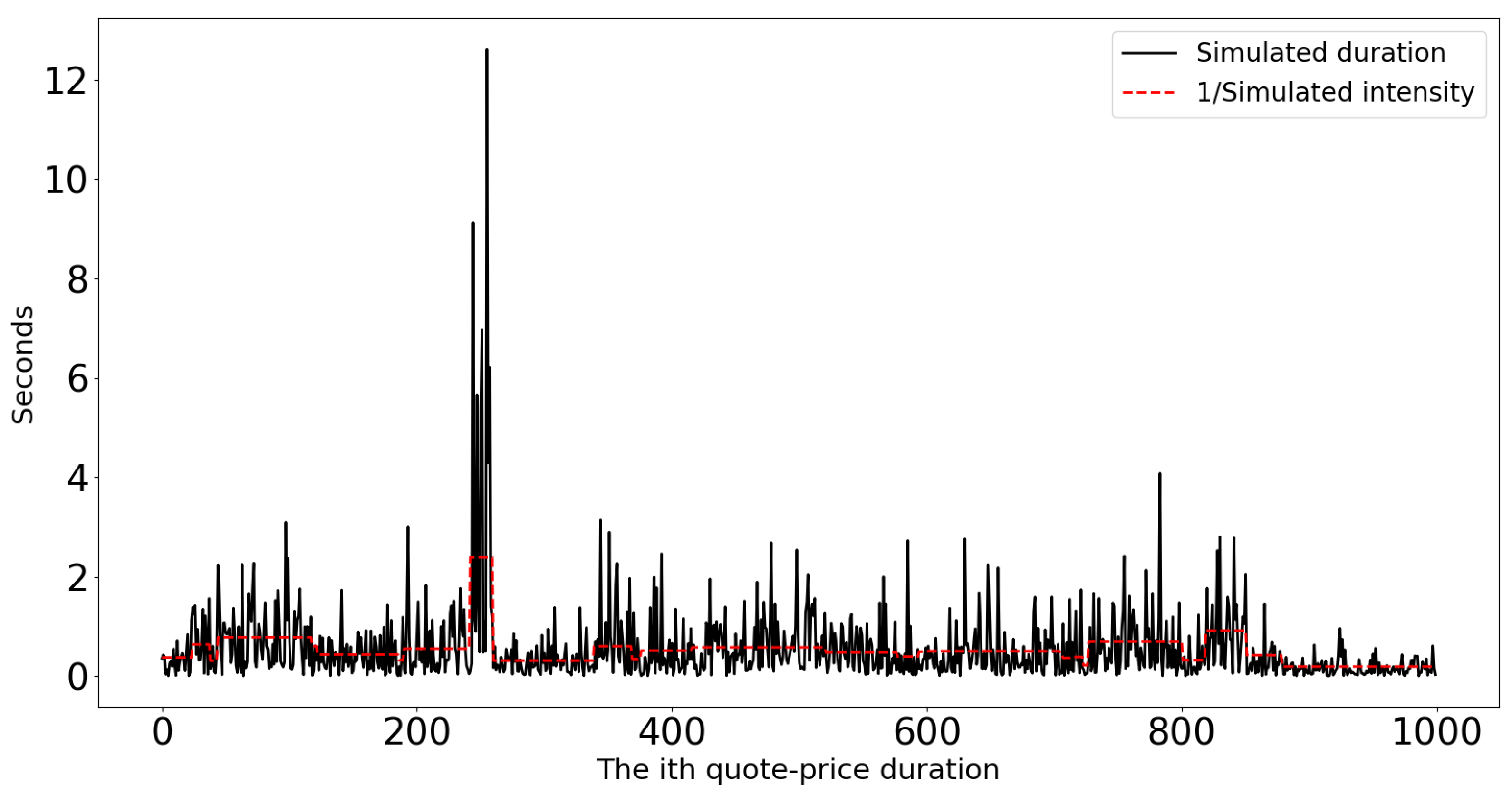
In order to validate the change-point model and the corresponding estimation algorithm, we first simulated data that provided us with the true values of model parameters for comparison. We have simulated 7000 points of price-change events, and the parameters are $\alpha =5.0$ (shape parameter in Gamma), $\beta =2.0$ (rate parameter in Gamma), and $p=0.018$ (the change point probability). Given this data generating process of the price-change intensity, we plot the simulated durations of quote-price changes in Figure 1. We also plot the inverse of simulated intensity ${\lambda }_t$, which is mean duration $m_t$ in Figure 1. From the graph, we can observe that there is a large variation of event duration, i.e., the longest duration is more than 12 s, while the short duration is about $1\times {10}^{-3}$ s. This means that sometimes it takes a couple of seconds for a change in quote price, while sometimes it only needs a millisecond for a price change. Clearly, the volatility of this simulated quote price is not constant.

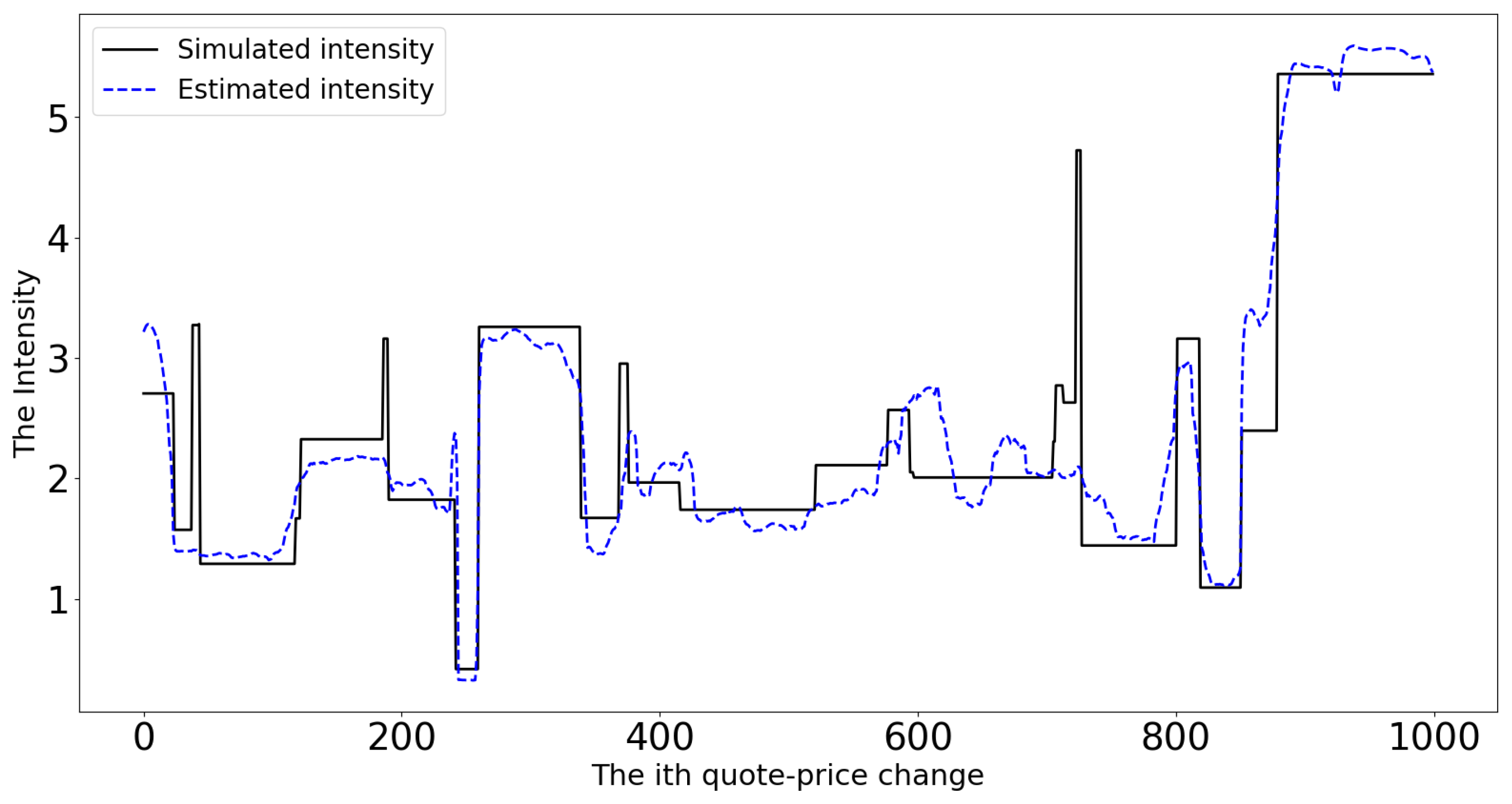
We use the estimation method shown in Section 3.1 to estimate model parameters. We have performed our estimation by using the first 1000 points, 4000 points, and the entire sample, respectively. The results are presented in

Table 1. Estimation results for the simulated data, which has $\alpha =5.0$, $\beta =2.0$, and $p=0.018$.

	$\widehat{\mathit{\alpha }}$	$\widehat{\mathit{\beta }}$	$\widehat{\mathit{p}}$
1000 points	3.47	1.51	0.030
4000 points	3.91	1.67	0.021
7000 points	4.10	1.77	0.019

, and we observe that the estimations are close to real values, especially for the large sample. Moreover, we have plotted simulated intensities and estimated intensities, together with simulated inter-trade durations in Figure 2 for $N_{sample}=7000$, and we find that the estimated intensities of price changes are also close to the ones in the simulated path.

4. Data Environment

Our data are downloaded from LOBSTER (https://lobsterdata.com/ accessed on 2 February 2018), which provides high-quality LOB data of all Nasdaq stocks from June 2007. The LOB data reconstructed by LOBSTER are based on Nasdaq’s Historical TotalView-ITCH data, i.e., the historic record of what Nasdaq calls. LOBSTER simultaneously generates two files for each active trading day of a selected ticker. One is a ‘message’ file, which contains indicators for the type of event causing an update of LOB in the requested price range. The other is an ‘orderbook’ file, which records the ask and bid quotes of LOB at the time when the ‘message’ file is updated.

Table 2. The message file and order book file of LOBSTER data.

Panel A: message file
Time (s)		Event Type	Order ID		Size	Price	Direction
⋮		⋮	⋮		⋮	⋮	⋮
35,101.685250		3	24,832,000		100	2,555,000	−1
35,101.685251		1	24,836,387		100	2,554,700	−1
35,101.685879		1	24,836,403		100	2,550,800	1
⋮		⋮	⋮		⋮	⋮	⋮
Panel B: order book file
Ask Price 1	Ask Size 1	Bid Price 1	Bid Size 1	Ask Price 2	Ask Size 2	Bid Price 2	Bid Size 2
⋮	⋮	⋮	⋮	⋮	⋮	⋮	⋮
25,550,00	300	2,550,700	100	2,555,100	100	2,550,500	100
2,554,700	100	2,550,700	100	2,555,000	300	2,550,500	100
2,554,700	100	2,550,800	100	2,555,000	300	2,550,700	100
⋮	⋮	⋮	⋮	⋮	⋮	⋮	⋮

shows a sample of LOB ‘messages’ and ‘orderbook’ files of AMZN on 2 January 2013. We show three events of the LOB. In panel A of Table 2, which is the ‘messages’ file, type 3 event and type 1 event represent a deletion and submission of a limit order, respectively. The direction ‘−1’ means the order event from the ask side, and ‘1’ denotes the bid-side order. In the meantime, the ‘orderbook’ file in panel B of Table 2 records the ‘shape’ of LOB after these three events. From this, we can observe that after submission of a new order at the bid side with a higher price than the existing best bid, the new best bid changes from 2550700 to 2550800, i.e., $255.07 to $255.08.

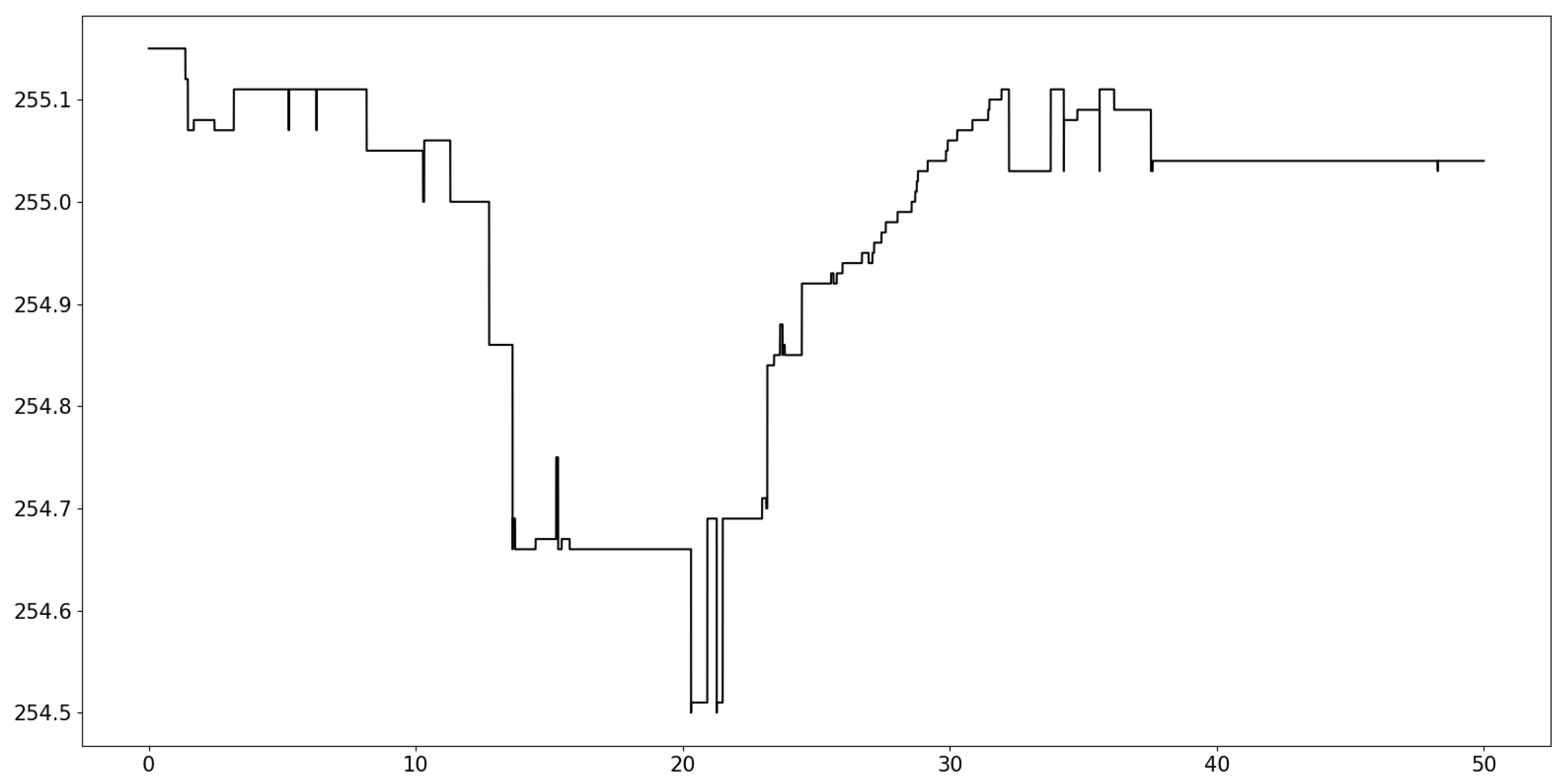
Figure 3 plots the evolution of quote price at the best bid in the first 50 s of AMZN stock on 2 January 2013. From this, we can observe that there is non-constant variation of bid price, with some intervals being much more volatile than others. A liquidity demander with 1 s of latency will encounter a high uncertainty and cost when she posts a (sell-side) market order at $t=20$ or $t=30$, compared with the entering time at $t=40$. Therefore, we need a method to effectively quantify the volatility of the quote price at any time and also the cost of demand for traders with different trading latencies.

5. Model Fitness and In-Sample Analysis

5.1. Model Fit and Instantaneous Volatility

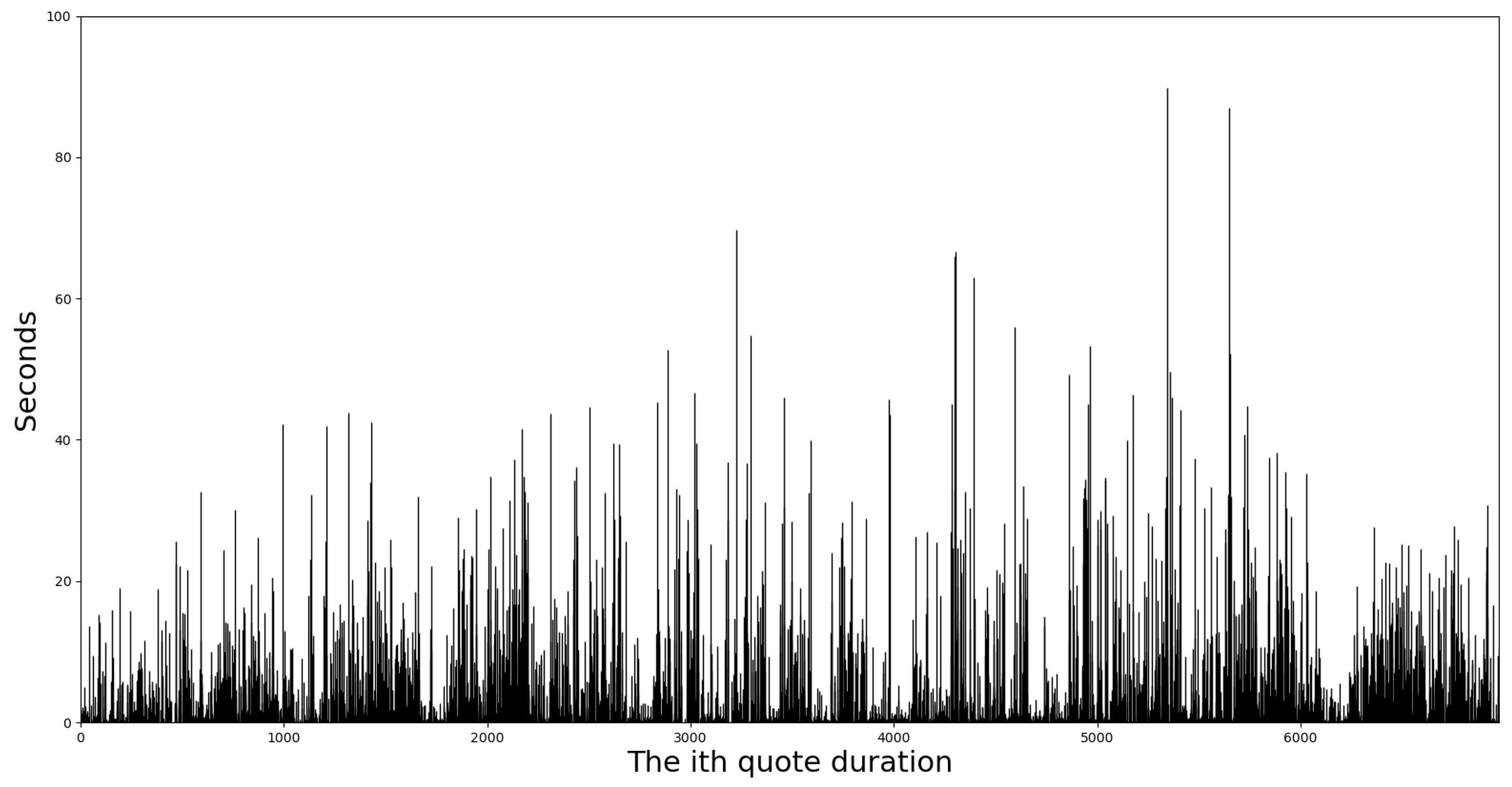
We use AMZN LOB data on 2 January 2013 to illustrate model fitness and to obtain the measurement of quote volatility. We choose the threshold of price change as 3 cents, which is three times the minimum unit of quote price. In Figure 4, we plot the series of quote-price duration (at the best bid level) of AMZN stock on 2 January 2013, given the threshold of price change as 3 cents. There is a large variation for this level of price duration. The shortest duration is ${10}^{-5}$ s, while the longest duration is about 80 s.

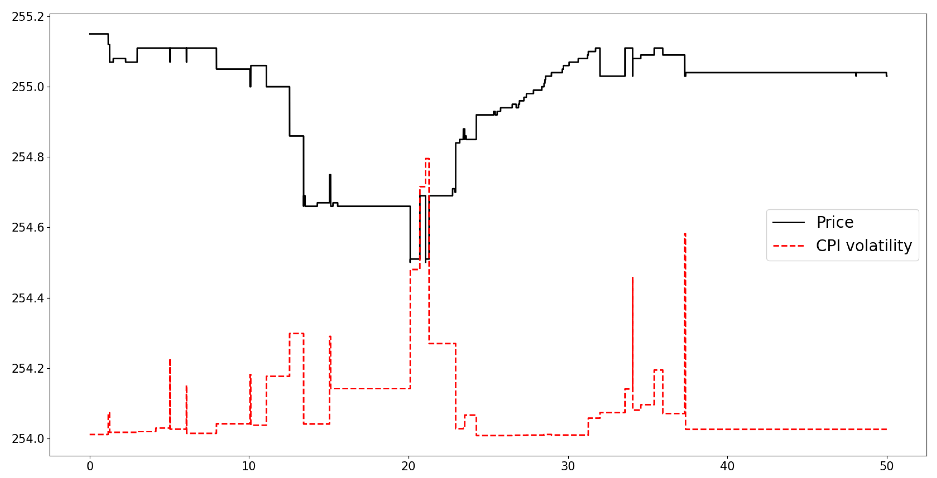
We first use our change-point intensity model (CPI) for estimation. The results are $\widehat{\alpha }=0.25$, $\widehat{\beta }=0.006$, and $\widehat{p}=0.34$. Moreover, we can infer underlying intensities ${\left\{{\lambda }_t\right\}}_{1,\dots ,N}$ according to Equation (26). The instantaneous volatility can be derived according to Equation (1). Specifically, for time $t\in [t_i,t_{i+1})$, we have the following:

$${\sigma }^2(t)=\lambda (t_i){\left(\frac{\delta }{p(t_i)}\right)}^{2}t\in [t_i,t_{i+1})$$

because, in the change-point model, intensity is assumed to be constant between two events. In Figure 5, we plot the fitted instantaneous quote volatility of the best bid price for the first 50 s of AMZN on the trading day of 2 January 2013. From the graph, we can observe that instantaneous quote volatility jumps to a high level when the quote price changes dramatically in a short time. On the other hand, volatility stayed at a low level if the quote price maintains fixed or changes steadily.

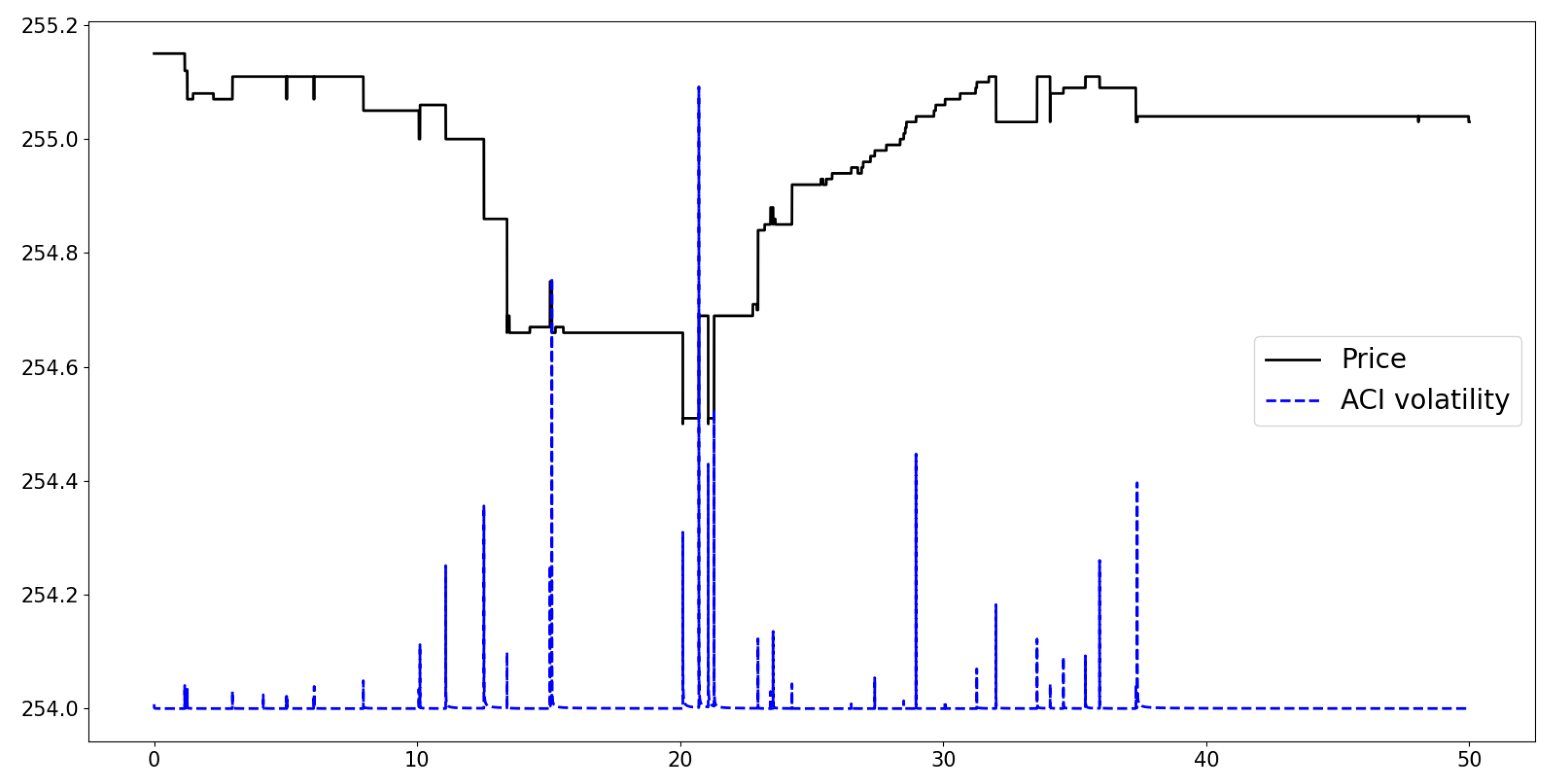
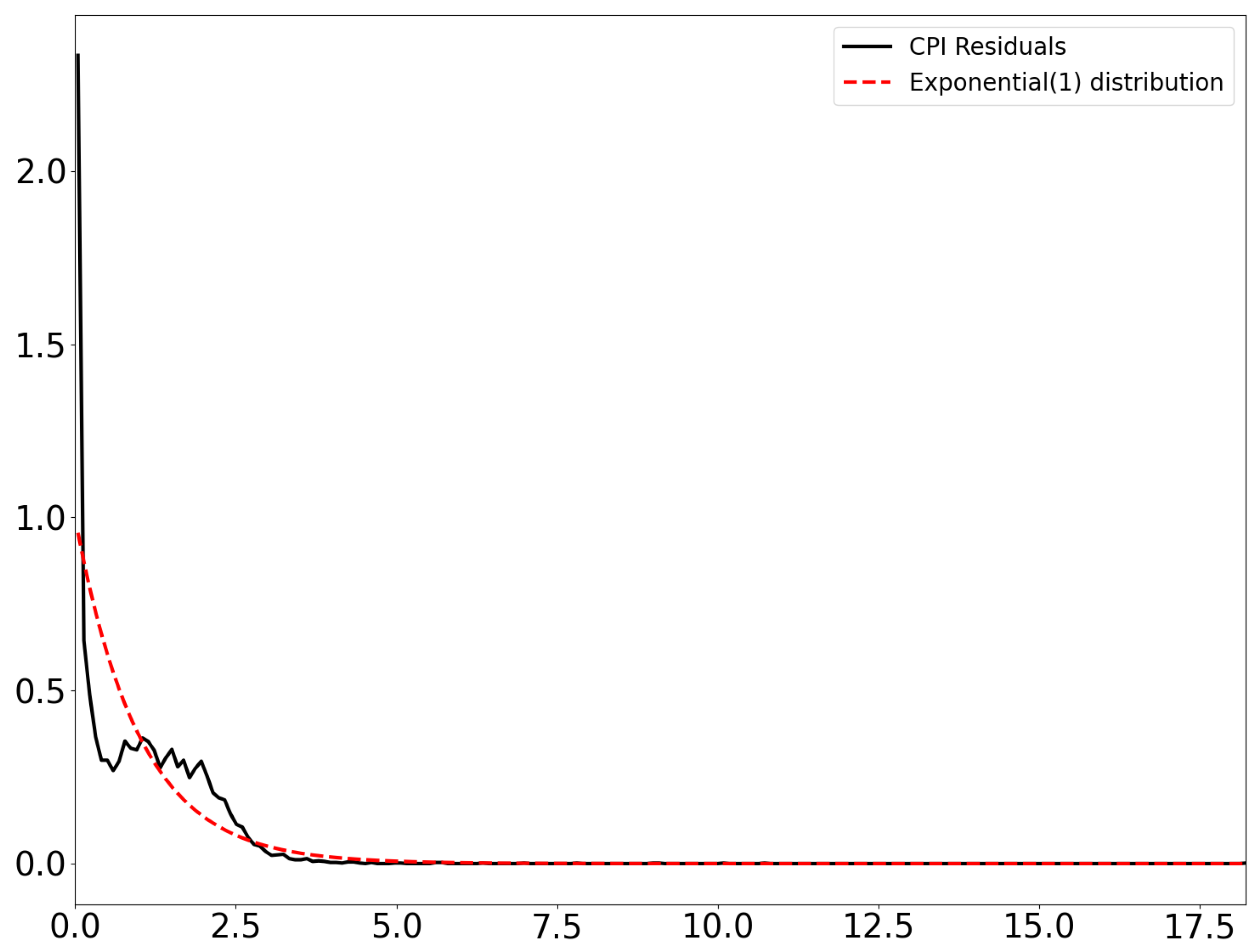
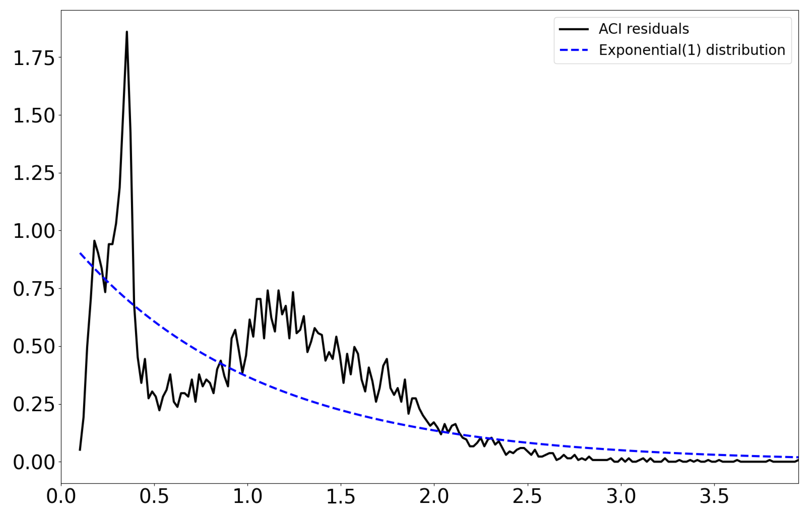
Moreover, we supplement the quote volatility estimation results by the ACI model in Figure 6, from which we can observe that ACI volatility exhibits strong spikes at the point when the quote price suddenly changes over a threshold. Furthermore, we provide the comparison between the models’ fitted residuals in Figure 7 and Figure 8. According to the property of the integrated intensity function shown in Equation (2) and the mixture of exponential expression in Equation (3), we should have the model’s fitted residuals follow an Exponential(1) distribution. From the results, we can clearly observe that the CPI model has a better result in terms of fitness.

5.2. Integrated Variance and Cost of Demand

Denote $p_t$ as the logarithm price of the best bid quote or the best ask quote. Under the assumption of no arbitrage, we suppose it follows a continuous semi-martingale process:

$$p_t=p_0+{\displaystyle {\int }_0^t}\mu (\tau )d\tau +{\displaystyle {\int }_0^t}\sigma (\tau )d{W}_{\tau }$$

where W denotes a standard Wiener process, $\mu (\tau )$ is a finite càdlàg drift process, and $\sigma (\tau )$ is an adapted càdlàg volatility process associated with the instantaneous conditional mean and volatility of the corresponding return.

The integrated variance over a interval $[0,t]$ is as follows:

$$IV(0,t):={\displaystyle {\int }_0^t}{\sigma }^2(\tau )d{W}_{\tau },$$

which also equals to the quadratic variation of a process corresponding to the sum of its squared increments measured on infinitesimal intervals. Hence, it is a natural quantity reflecting the riskiness of an asset over a given time span. Thus, we can use the derived the instantaneous volatility to calculate the the integrated variance.

For liquidity demanders with different trading latency ${\mathsf{\Delta }}_i$, the integrated variances are specifically as follows.

$$IV(t,t+{\mathsf{\Delta }}_i):={\displaystyle {\int }_t^{t+{\mathsf{\Delta }}_i}}{\sigma }^2(\tau )d{W}_{\tau }.$$

Therefore, the trading cost not only depends on latency ${\mathsf{\Delta }}_i$ but also on the magnitude of the (instantaneous) volatility over the interval. In

Table 3. The integrated variances for different traders that calculated for AMZN stock on 2 January 2013.

Latency	Mean	S.D.	Min.	25%	Median	75%	Max.
0.01 S.	$7.6\times {10}^{-5}$	$1.1\times {10}^{-4}$	$3.0\times {10}^{-6}$	$2.0\times {10}^{-5}$	$2.6\times {10}^{-5}$	$8.1\times {10}^{-5}$	$8.0\times {10}^{-4}$
1 S.	$7.5\times {10}^{-3}$	$1.0\times {10}^{-2}$	$3.0\times {10}^{-6}$	$2.2\times {10}^{-3}$	$2.6\times {10}^{-3}$	$9.7\times {10}^{-3}$	$5.1\times {10}^{-2}$
5 S.	$3.5\times {10}^{-2}$	$3.8\times {10}^{-2}$	$3.0\times {10}^{-6}$	$1.1\times {10}^{-2}$	$1.5\times {10}^{-2}$	$4.9\times {10}^{-2}$	$1.3\times {10}^{-1}$

, we calculate the integrated variance for three types of trades, with trading latency of 0.01 s, 1 s, and 5 s, respectively. Clearly, a low-latency trader who has speed advantages in sending orders will encounter a lower risk to obtain her liquidity. For example, the mean value of the volatility of the transaction prices for a trader whose trading latency is 5 s is 0.035, while the value for a trader whose trading latency is 0.01 s is just $7.6\times {10}^{-5}$.

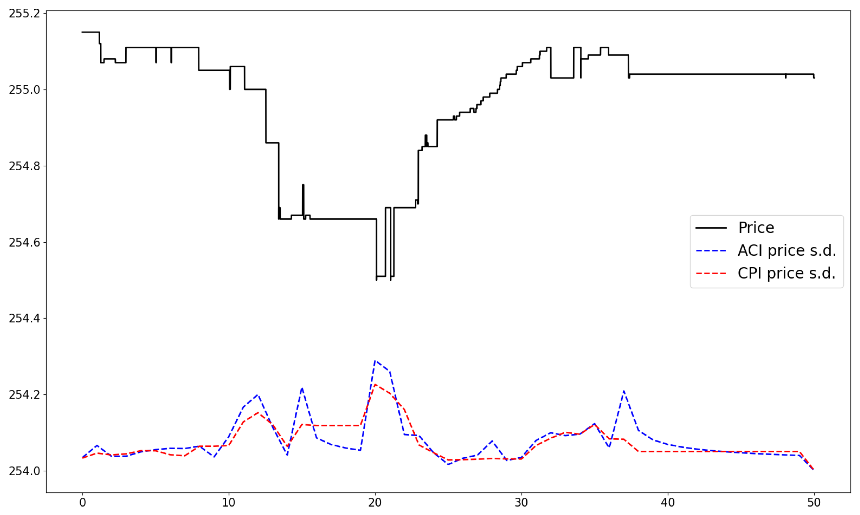
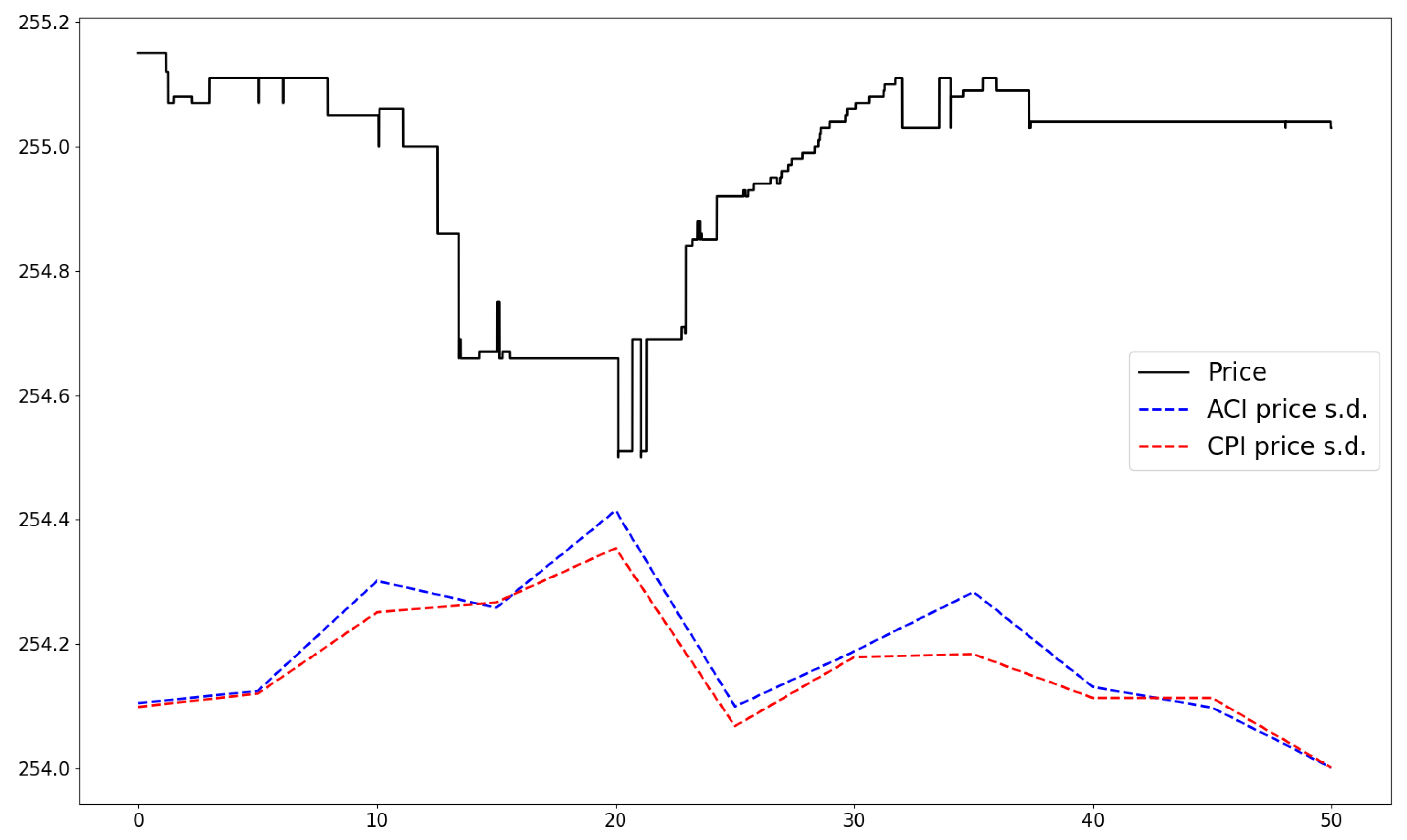
Moreover, in the below figures (Figure 9, Figure 10 and Figure 11), we plot the fitted standard deviation (the square root of the integrated variance) of the bid price for the AMZN stock on 2 January 2013 in the first 50 s for three types of traders, for which their trading latencies are 0.01 s, 1 s, and 5 s, respectively. Compared with the ACI model, the price standard deviation estimated from our CPI model is relatively smooth, especially for the low-latency environment, which helps us to be more effective in evaluating the dynamics of quote volatility for HF traders. As the the evaluating time window increases, say the price standard deviation for 5 s, both models obtain similar results.

We can quantify the cost of demand for a specific type of traders at different time points when initiating her orders. We use the price standard deviation as the cost of demanding liquidity. For example, for a trader whose trading latency is 1 s, she will suffer price uncertainty of USD 0.089 when she enters the market at $t=10$ s. While when this trader enters the market at $t=20$ s, the price uncertainty of her transaction price is about USD 0.289.

6. Out-of-Sample Performance and Model Prediction Power

At last, we want to examine the out-of-sample performance of our CPI model. However, it is hard to predict the volatility directly and to observe the model’s performance because actual volatility is unobserved. Therefore, we only predict the duration length for the next price change as the actual price-change duration is known to us. When the duration for the change of quote price is long, quote volatility is low. On the other hand, when the duration for the change of quote price is short, quote volatility should be high.

We use one-step-ahead forecasting based on the model’s in-sample estimation results. Specifically, for the quote prices (at the best bid) of the AMZN stock on 2 January 2013, we use the first 4000 data points (which are the 4000 events of price changes) for parameter estimation and perform a one-step-ahead prediction for the remaining observations of price durations. The expected price-change duration for the quote price can be derived as follows.

$$\begin{array}{ccc}\hfill {\mathrm{E}}_t(y_{t+1})& =& \frac{1}{{\mathrm{E}}_t({\lambda }_{t+1})}\hfill \\ & =& \frac{1}{\widehat{p}·\widehat{{\lambda }_t}+(1-\widehat{p})·\frac{\widehat{\alpha }}{\widehat{\beta }}}.\hfill \end{array}$$

(27)

This is because, in the CPI model, the intensity for the next price change either retains its past value ${\lambda }_t$ (with probability $\widehat{p}$) or renews from the Gamma distribution (with probability 1 − $\widehat{p}$), and the mean value of the Gamma distribution is $\frac{\widehat{\alpha }}{\widehat{\beta }}$.

We test the model’s out-of-sample performance by using the Mincer–Zarnowitz ordinary least squares (OLS) regressions.

$$y_{t+1}={\beta }_0+{\beta }_1{\mathrm{E}}_t(y_{t+1})+{\mu }_t,$$

(28)

where ${\beta }_0$ is the regression intercept, ${\beta }_1$ is the regression coefficient for ${\mathrm{E}}_t(y_{t+1})$, and ${\mu }_t$ is the regression error term.

Moreover, we compare the model’s performance with the ACI model, and the results are shown in

Table 4. Mincer–Zarnowitz OLS results for CPI and ACI models.

	CPI Model	ACI Model
${\beta }_0$	−0.241	−5.568
	(−2.735)	(−10.953)
${\beta }_1$	4.236	12.614
	(78.800)	(18.310)
$R^2$	0.676	0.101
N	2974	2974

. From the results, we can observe that coefficients ${\beta }_1$ are significantly positive in both models, suggesting that the predictions from both the CPI and ACI models can explain the variation of the real value of price-change durations. Nevertheless, our CPI model is significantly better in terms of prediction power because the R-squared in the fitting of CPI model is much higher.

7. Conclusions

This paper has proposed a new method to measure the volatility of quote prices in the limit order market, which is important to quantify the cost of demanding liquidity in the HF trading environment. We use the point process to describe price-change events that occur at the best quote level (at the best bid or the best ask), and volatility is measured based on the inference of price-change intensity according to realized price-change durations. In particular, we resort to the change-point model proposed by Lai et al. [23] to describe the dynamics of price-change intensity and name it as the change-point intensity (CPI) model. In the model, the underlying price-change intensity follows a Markov process, i.e., either maintains its past value or renews from a Gamma distribution. Thus, we can use the data of price-change durations to infer the underlying price-change intensity and further calculate quote volatility based on the method proposed by Engle and Russell [5].

We apply the CPI model to study the quote volatility of the AMZN stock on 2 January 2013. Specifically, we choose the threshold of price change as 3 cents to define the price-change event and construct the series of price-change durations. The instantaneous quote volatility at any time of the trading day can be derived from the estimated price-change intensity by our CPI model. Furthermore, we have calculated the cost of demand for traders with different trading latency based on the integrated variance. In addition, we compare both the in-sample fitness and out-of-sample prediction power with the benchmark ACI model by Russell [18], and the results suggest that our model performs better.

Our work has made progress in modeling HF quote volatility. Nonetheless, it leaves much room for future development. The current CPI model is a univariate structure that studies the dynamics of quote volatility itself. We can further extend it by incorporating other factors in determining the changes of quote volatility. This can be performed by setting intensity renewal probability p to be time-varying and to be driven by some other factors.

References

1. Hasbrouck, J. High-frequency quoting: Short-term volatility in bids and offers. J. Financ. Quant. Anal. 2018, 53, 613–641. [Google Scholar] [CrossRef]
2. Hasbrouck, J.; Saar, G. Low-latency trading. J. Financ. Mark. 2013, 16, 646–679. [Google Scholar] [CrossRef]
3. Bauwens, L.; Hautsch, N. Modelling financial high frequency data using point processes. Handb. Financ. Time Ser. 2009, 1, 953–979. [Google Scholar]
4. Hautsch, N. Econometrics of Financial High-Frequency Data; Springer Science & Business Media: Berlin/Heidelberg, Germany, 2011. [Google Scholar]
5. Engle, R.F.; Russell, J.R. Autoregressive conditional duration: A new model for irregularly spaced transaction data. Econometrica 1998, 1, 1127–1162. [Google Scholar] [CrossRef]
6. Hautsch, N. Modelling Irregularly Spaced Financial Data: Theory and Practice of Dynamic Duration Models; Springer Science & Business Media: Berlin/Heidelberg, Germany, 2011. [Google Scholar]
7. Žikeš, F.; Baruník, J.; Shenai, N. Modeling and forecasting persistent financial durations. Econom. Rev. 2017, 36, 1081–1110. [Google Scholar] [CrossRef]
8. Yang, J.; Li, Z.; Chen, X.; Xing, H. Modeling inter-trade durations in the limit order market. New Adv. Stat. Data Sci. 2017, 1, 259–276. [Google Scholar]
9. Chen, F.; Diebold, F.X.; Schorfheide, F. A Markov-switching multifractal inter-trade duration model, with application to US equities. J. Econom. 2013, 177, 320–342. [Google Scholar] [CrossRef] [Green Version]
10. Abergel, F.; Jedidi, A. Long-time behavior of a Hawkes process–based limit order book. SIAM J. Financ. Math. 2015, 6, 1026–1043. [Google Scholar] [CrossRef]
11. Swishchuk, A.; Huffman, A. General compound Hawkes processes in limit order books. Risks 2020, 8, 28. [Google Scholar] [CrossRef] [Green Version]
12. Morariu-Patrichi, M.; Pakkanen, M.S. State-dependent Hawkes processes and their application to limit order book modelling. Quant. Financ. 2021, 1, 1–21. [Google Scholar] [CrossRef]
13. Li, Z.; Xing, H.; Chen, X. A multifactor regime-switching model for inter-trade durations in the limit order market. arXiv 2019, arXiv:1912.00764. [Google Scholar] [CrossRef] [Green Version]
14. Cho, D.C.; Frees, E.W. Estimating the volatility of discrete stock prices. J. Financ. 1988, 43, 451–466. [Google Scholar] [CrossRef]
15. Gerhard, F.; Hautsch, N. Volatility estimation on the basis of price intensities. J. Empir. Financ. 2002, 9, 57–89. [Google Scholar] [CrossRef] [Green Version]
16. Tse, Y.-K.; Yang, T.T. Estimation of high-frequency volatility: An autoregressive conditional duration approach. J. Bus. Econ. Stat. 2012, 30, 533–545. [Google Scholar] [CrossRef]
17. Hong, S.Y.; Nolte, I.; Taylor, S.; Zhao, V. Volatility estimation and forecasts based on price durations. J. Financ. Econom. 2021, nbab032. [Google Scholar] [CrossRef]
18. Russell, J.R. Econometric Modeling of Multivariate Irregularly-Spaced High-Frequency Data. Manuscript, GSB, University of Chicago. 1999. Available online: http://citeseerx.ist.psu.edu/viewdoc/download?doi=10.1.1.202.486&rep=rep1&type=pdf (accessed on 1 December 2021).
19. Bauwens, L.; Hautsch, N. Stochastic conditional intensity processes. J. Financ. Econom. 2006, 4, 450–493. [Google Scholar] [CrossRef]
20. Hall, A.D.; Hautsch, N. Modelling the buy and sell intensity in a limit order book market. J. Financ. Mark. 2007, 10, 249–286. [Google Scholar] [CrossRef]
21. Bowsher, C.G. Modelling security market events in continuous time: Intensity based, multivariate point process models. J. Econom. 2007, 141, 876–912. [Google Scholar] [CrossRef] [Green Version]
22. Box, G.E.; Tiao, G.C. Intervention analysis with applications to economic and environmental problems. J. Am. Stat. Assoc. 1975, 70, 70–79. [Google Scholar] [CrossRef]
23. Lai, T.L.; Liu, H.; Xing, H. Autoregressive models with piecewise constant volatility and regression parameters. Stat. Sin. 2005, 1, 279–301. [Google Scholar]
24. Lancaster, T. The Econometric Analysis of Transition Data; Cambridge University Press: Cambridge, UK, 1990. [Google Scholar]
25. Daley, D.J.; Vere-Jones, D. An Introduction to the Theory of Point Processes: Volume I: Elementary Theory and Methods; Springer: New York, NY, USA, 2003. [Google Scholar]
26. Barndorff-Nielsen, O.E.; Shiryaev, A.N. Change of Time and Change of Measure; World Scientific Publishing Company: Singapore, 2015. [Google Scholar]
Figure 1. The simulated quote-price change durations and price-change intensities (first 1000 points).
Mathematics 10 00634 g001
Figure 2. Comparison between actual intensity in the simulation and estimated intensity from model estimation.
Mathematics 10 00634 g002
Figure 3. The evolution of best bid price in the first 50 s of AMZN stock on 2 January 2013.
Mathematics 10 00634 g003
Figure 4. The quote price duration of the best bid price for the AMZN stock on 2 January 2013.
Mathematics 10 00634 g004
Figure 5. The instantaneous quote volatility of the best bid price for AMZN stock on 2 January 2013 calculated by the change-point model.
Mathematics 10 00634 g005
Figure 6. The instantaneous quote volatility of the best bid price for AMZN stock on 2 January 2013 calculated by the ACI model.
Mathematics 10 00634 g006
Figure 7. The distribution of duration residuals of CPI.
Mathematics 10 00634 g007
Figure 8. The distribution of duration residuals of ACI.
Mathematics 10 00634 g008
Figure 9. The fitted 0.01 s price standard deviation of the best bid price for AMZN stock on 2 January 2013.
Mathematics 10 00634 g009
Figure 10. The fitted 1 s price standard deviation of the best bid price for AMZN stock on 2 January 2013.
Mathematics 10 00634 g010
Figure 11. The fitted 5 s price standard deviation of the best bid price for AMZN stock on 2 January 2013.
Mathematics 10 00634 g011