Abstract
In this article, an approach to achieve the anti-disturbance fault-tolerant constrained consensus is proposed for time-delay faulty multi-agent systems under semi-Markov switching topology. Firstly, an observer based on the coupled disturbance and fault information is designed to estimate the disturbance and failure at the same time. Next, because of the conservatism of the traditional control method, a new performance index is constructed to replace the zero initial condition by making use of initial conditions. Then, the time-varying transfer rate is expressed as a convex combination by using the boundedness of transfer rate, so as to solve the numerical solution problem of time-varying transfer rate. On this basis, according to the performance requirements, an anti-disturbance fault-tolerant constrained consensus strategy is proposed. Finally, simulation results are given to verify the feasibility of the approach.
Keywords:
time-delay multi-agent system; fault-tolerant constrained consensus; disturbance observer; H∞ control; semi-Markov switching topology MSC:
93A16
1. Introduction
In the past years, it is obvious that the consensus problem has gradually become one of the most active topics in the field of multi-agent systems. It has attracted extensive research in the fields of building automation [], smart grids [], intelligent transportation [], underwater exploration [], cooperative search [], etc. However, considering security and the particularity of tasks, the agent state is often constrained in practical applications. For example, due to terrain constraints, the agent can only move within constrained areas. Therefore, the constrained consensus of many systems has attracted the attention of more and more researchers; see related articles [,,,,,]. A new distributed primal–dual augmented (sub) gradient algorithm is studied in reference [], and the distributed constrained optimization and consensus problem in uncertain networks via proximal minimization are discussed in [].
Furthermore, in many practical multi-agent systems, considering the limitations and disturbances of obstacles and communication range, the communication topology between agents may change randomly. In order to be more in line with the actual situation, it is a good choice to model the random change in communication topology as a semi-Markov process. The synchronization problem of complex networks with semi-Markov switching topology has attracted more attention of some scholars; see [,]. The change in system topology will affect the implementation of constrained consensus, which is one of the research purposes of this article.
On the other hand, in the actual multi-agent system, faults, external disturbances and communication delays are also inevitable, which will lead to the destruction of the system performance. In order to ensure the safety and reliability of the closed-loop system, it is feasible for fault-tolerant control to be used; see [,,,,,,]. By using the adjacency matrix information, a robust adaptive fault-tolerant protocol is proposed to compensate the actuator bias fault and the partial loss of actuator effectiveness fault in []. In [], the consensus problem of nonlinear multi-agent systems with multi-actuator failure and uncertainty is analyzed. Ref. [] proposed a strategy to solve the bipartite consensus of high-order multi-agent systems with unknown time-varying disturbances. The disturbances are estimated by designing the adaptive law for unknown parameters. Additionally, the proposed adaptive control method can realize consensus control. In [], a nonlinear disturbance observer is proposed to estimate the disturbances to better realize the consensus of linear multi-agent systems. In [], a disturbance observer with adaptive parameters is designed for nonlinear multi-agent systems to suppress the total disturbance, including unknown external disturbances and deviation faults. Ref. [] proposed an accelerated algorithm to solve the linear quadratic optimal consistency problem of multi-agent systems. Ref. [] studied the global consensus problem of a class of heterogeneous multi-agent systems, but both of them ignore the impact of external interference and actuator failure on the constraint consistency of multi-agent systems. Most of the above studies focus on consensus, but there are few studies on anti-disturbance constrained consensus, especially the existence of disturbance and fault coupling in a time-delay system. This is the second motivation of this article.
This article studies the fault-tolerance constrained consensus for time-delay multi-agent systems with external disturbances and faults based on semi-Markov switching topology. The main contributions of this article are as follows:
(a) Owing to the external disturbances and actuator failures being coupled in time-delay multi-agent systems, inspired by [,,,], a new disturbance observer can be used to estimate disturbance and fault concurrently.
(b) In order to make the influence of semi-Markov switching topology weaken, taking [] as the starting point, the time-varying transfer rate is expressed as a convex combination by using the boundedness of transfer rate, so as to solve the numerical solution problem of time-varying transfer rate.
(c) For actuator failures and external disturbances, a novel anti-disturbance fault-tolerant control algorithm is provided to ensure the stability of multi-agent systems, as well as to achieve a consensus on the anti-disturbances’ dynamic fault tolerance constraints.
Notation: denotes the m-dimensional Euclidean space; denotes the set of vectors and matrices of appropriate dimension; and for a symmetric matrix, ‘∗’ denotes the elements below the main diagonal, which are determined by the matrix symmetry. Let be the block-diagonal matrix with matrices on its principal diagonal; for a given matrix A, denotes its transpose; ⊗ denotes the Kronecker product of matrix; stands for the identity matrix of ; and is a column vector with all entries being 1. we use to represent the Euclidean norm of vectors or matrices.
2. Preliminaries and Problem Formulation
2.1. Graph Theory
A vertices set , an edges set and an adjacency matrix make up graph . stands for the projection of the vector x on the closed convex set . Use for each edge, which means that node is a neighbor of , or node is a neighbor of . When the graph is undirected, for all p, q. The adjacency matrix has the following characteristics: (), and the Laplacian matrix can be represented by . Furthermore, the interactive topology of semi-Markov topology switching is noted as: , , where is a switching signal, which is controlled by semi-Markov process. The evolution of semi-Markov processes is determined by the following transition probability:
In the equation above, the transition rate is time-varying and dependent on h, where h is called sojourn time, which represents the duration between two jumps.
2.2. Problem Formulation
Given the multi-agent systems with the following dynamics:
where , stands for the control input. n is the number of the agent. stands for the state of agent. is the external disturbance in the system. Considering the partial failure of actuator, the model can be described as
which denotes the output signal from the dth actuator of the pth agent. d represents the numbers of actuator channels. and stand for the upper and lower bounds of , respectively. When , it represents that there is no failure of the dth actuator. If , it indicates that the dth actuator is partially faulty.
For each agent described by (1), a variable represents the disturbance of the pth agent to be rejected, and it can be described by the following exosystem:
where is a known constant matrix, and the matrix of each agent can be different.
Our ultimate goal is to make the anti-disturbance fault-tolerant constrained consensus of multi-agent systems (1), achieved by designing an appropriate controller in the case of semi-Markov topology switching. The following definition and lemmas are recalled:
Definition 1
([]). When the state of agent p and the state of any other agent q satisfy the following equation, the multi-agent system is said to have constrained consensus:
Note that stands for the projection of the vector x on the closed convex set , and is the vertex set defined in the above graph theory.
Lemma 1
(Schur complement []). Given a symmetric matrix
the following statements are equivalent:
Lemma 2
([]). Let ℘= and and be real matrices of appropriate dimensions with satisfying , then , if and only if there exists some such that .
Lemma 3
([]). The transition rate (h) of semi-Markov is time-varying. If its bound is , the following formulas are recalled:
3. Distributed Fault-Tolerant Protocol Design
In this section, the following control law is designed for systems with constant communication delay :
where represents the controller gain that we need to design. stands for the estimation of the disturbance .
In addition, in an actual system, disturbance and fault are often coupled together, so disturbance observer and fault estimation cannot be designed separately. Therefore, we design the following interconnected disturbance observer and fault adaptive law
where is a subsidiary variable, and is the gain of the observer and can be calculated to obtain it. is the estimation of the failure . , , is a positive number. stands for the projection of the vector x on the closed convex set .
Next, we solve the anti-disturbance fault-tolerant constrained consensus problem of system (1) under semi-Markov switching topology.
4. Main Result
Theorem 1.
For the undirected and connected graph and multi-agent system (1), let the attenuation level Given partial failure coefficient and matrix H, the whole system can achieve anti-disturbance fault-tolerant constrained consensus with an disturbance attention level γ under the control law (4) and disturbance observer (5) (6) if the existence of matrices , , and with suitable dimensions, suitable parameter , , , and a positive number make the following matrix inequalities hold:
where
Proof.
Choose a Lyapunov function, shown as follows:
where
The weak infinitesimal operator of can be calculated as follows:
Define and the following results can be obtained directly:
Therefore, considering the above analysis, using augmented vector and adaptive law (6), we can obtain the following results:
where . See Appendix A for the specific derivation process of Equation (9). It is necessary to ensure that zero initial conditions are met when we use the traditional control theory. This situation will bring some conservatism, and the following performance requirements are built based on initial conditions:
where
Therefore, define , then we have
where and
where
However, θ in Ξ is unknown. How to deal with it? The answer is that we can utilize to reduce its conservation, where
Therefore, the following formula can be obtained from (11):
where
By utilizing (10), (12) and Lemma 2, the following result can be obtained:
Based on Lemma 2, (13) can be converted to (14)
where
According to the above, if inequality (14) holds, we can obtain that , clearly. Next, we can obtain
See Appendix B for the detailed derivation process.
Combined and , when the linear matrix inequalities (14) and (8) are satisfied, , , . Therefore, the whole system can achieve anti-disturbance fault-tolerant constrained consensus with required performance indicators. But the above linear matrix inequality contains coupling terms, definition:
multiply matrices and on the left and right sides of some transformations are introduced to better illustrate the theorem:
From the above, we can obtain the linear matrix inequalities (7) and (8), and the controller gains can be obtained by . The proof of Theorem 1 is completed. □
Since the transition rate of the semi-Markov process in Theorem 1 is time-varying and difficult to solve, in order to solve this problem, we design the following theorem.
Theorem 2.
For the undirected and connected graph and multi-agent system (1), let the attenuation level The transition rate has upper and lower bounds. Given partial failure coefficient and matrix H. The whole system can achieve anti-disturbance fault-tolerant constrained consensus in the presence of time-delay and semi-Markov switching topology with an disturbance attention level γ under the control law (4) and disturbance observer (5) (6) if the existence of matrices , , and with suitable dimensions, suitable parameter , , , , and a positive number make the following matrix inequalities hold:
where:
Proof.
Based on the Lemma 3, the term can be split into portions: one is with the element δ, and the other is without the element δ. Note that and , then one has
That is to say
can be ensured by
Then
Note that
where
We have:
The following can be obtained from (16): is equivalent to , where is the determined constant.
- if , .
- if , .
where
So, is equivalent to Then, we define , . Linear matrix inequality (7) can be transformed into linear matrix inequality (15), and Theorem 2 is proved. □
5. Numerical Example
In this part, it is assumed that the dynamic interaction topology is semi-Markov switching and the semi-Markov process has three modes. Let us take four agents as examples. It is assumed that the weight of the first mode is 1 and that of the other two modes is 10. The corresponding topology is shown in Figure 1.
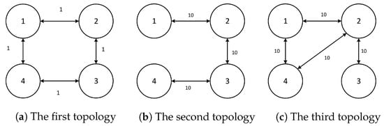
Figure 1.
Topological structure of three modes.
The corresponding Laplacian matrices of communication graph are described as follows:
It is assumed that the transition probability is bounded and satisfies:
In the simulation, the ranges of fault are set to , , and , . The communication delay is set to . Let
Based on Theorem 2, the calculated gain is as follows:
The simulation results of failure estimations and disturbance estimations of each agent are shown in Figure 2, Figure 3, Figure 4 and Figure 5. When there are disturbances and actuator failures in the system, the observer can quickly and accurately estimate the disturbances and judge the occurrence of the failure and, finally, estimate the failure rate of the actuator to improve the control effect.
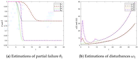
Figure 2.
Estimations of partial failure of actuators and disturbances (Agent 1).
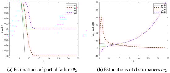
Figure 3.
Estimations of partial failure of actuators and disturbances (Agent 2).
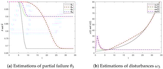
Figure 4.
Estimations of partial failure of actuators and disturbances (Agent 3).
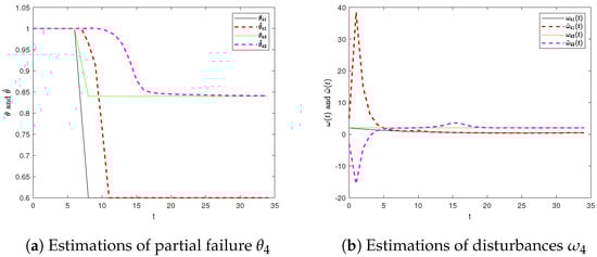
Figure 5.
Estimations of partial failure of actuators and disturbances (Agent 4).
Considering the influence of disturbance, actuator failures and the change in topology on the system, the trajectory of each agent is shown in Figure 6. Set Agent 1 and Agent 3 to fail when the time is 6 seconds, and Agent 2 and Agent 4 to fail at 7 seconds. The change in topology satisfies the semi-Markov process. In reference [], considering the influence of interference and actuator partial failure under the same conditions, the trajectory of each agent is shown in Figure 7. Obviously, in the absence of the application of the anti-disturbance fault-tolerant algorithm, due to the lack of strong robustness, once partial actuator failures and disturbances occur during system operation, and the control performance of the system will be greatly affected. Figure 8 shows the semi-Markov switching signal with three modes. We can clearly see in Figure 6 that under the influence of the fault-tolerant controller we designed, after constantly fluctuating the trajectory, all the agents finally reach the consensus point in Ω.
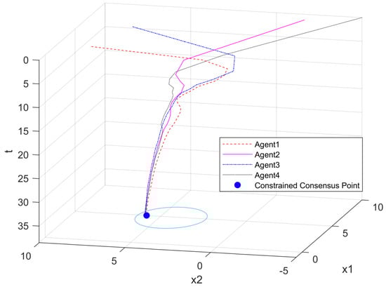
Figure 6.
All state trajectories of agents in our method.
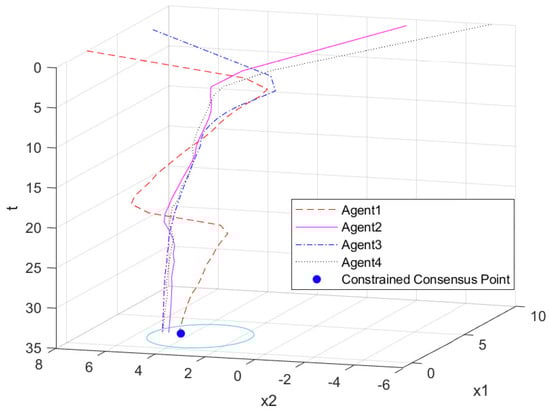
Figure 7.
All state trajectories of agents in other method.
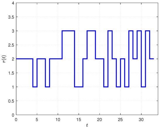
Figure 8.
Semi-Markov switching signal with three modes.
6. Conclusions
This article studies the consensus problem of anti-disturbance and fault-tolerant constraints of a time-delay multi-agent with semi-Markov topology switching. Firstly, a disturbance observer is designed to observe the external disturbance, and an adaptive law is designed to estimate the fault information combined with the known information of the system. Then, in order to bypass the zero initial condition in the harsh control method, a new performance index is designed by using the zero initial condition, and the time-varying problem is solved by using the upper and lower bounds of the time-varying transfer rate of the semi-Markov topology switching, so as to calculate the gain of the controller and disturbance observer. After this, the interference suppression level γ of the closed-loop system is given. Finally, the feasibility of our approach is verified by numerical simulations. Compared with the reference [], it is obvious that the multi-agent system has better anti-interference performance and fault tolerance in case of failure after the use of the anti-disturbance fault-tolerant control algorithm. This article mainly discusses the actuator failure fault of a constant time-delay multi-agent, and the number of agents is fixed. In future work, we can consider more complex fault models with time-varying delay and an uncertain number of agents in the system.
Author Contributions
Conceptualization, Y.C.; methodology, Y.C. and F.Z.; validation, Y.C., F.Z. and J.L.; formal analysis, F.Z. and J.L.; investigation, Y.C.; writing—original draft preparation, Y.C.; writing—review and editing, Y.C. All authors have read and agreed to the published version of the manuscript.
Funding
This work was supported by the Zhejiang Provincial Natural Science Foundation of China (No. LZ22F030008), the National Natural Science Foundation of China (No. 61733009), the Fundamental Research Funds for the Provincial Universities of Zhejiang (No. GK229909299001-012).
Institutional Review Board Statement
Not applicable.
Informed Consent Statement
Not applicable.
Data Availability Statement
Not applicable.
Conflicts of Interest
The authors declare no conflict of interest.
Appendix A
The detailed process of obtaining in Theorem 1 is as follows. First, according to the derivation of , , in Theorem 1, we have
Next, for ease of description, define the following augmented vectors as following:
Therefore, we have:
Then, combine (9) with adaptive law (6), and we can finally obtain the following results
where .
Appendix B
On the complex derivation process in the proof of theorem one
References
- Yang, R.; Wang, L. Development of multi-agent system for building energy and comfort management based on occupant behaviors. Energy Build. 2013, 56, 1–7. [Google Scholar] [CrossRef]
- Pipattanasomporn, M.; Feroze, H.; Rahman, S. Multi-agent systems in a distributed smart grid: Design and implementation. In Proceedings of the IEEE/PES Power Systems Conference and Exposition, Seattle, WA, USA, 15–18 March 2009; pp. 1–8. [Google Scholar]
- Adler, J.L.; Satapathy, G.; Manikonda, V.; Bowles, B.; Blue, V.J. A multi-agent approach to cooperative traffic management and route guidance. Transp. Res. Part Methodol. 2005, 39, 297–318. [Google Scholar] [CrossRef]
- Yan, Z.; Yang, Z.; Yue, L.; Wang, L.; Jia, H.; Zhou, J. Discrete-time coordinated control of leader-following multiple AUVs under switching topologies and communication delays. Ocean. Eng. 2019, 172, 361–372. [Google Scholar] [CrossRef]
- Jin, X.; Wang, S.; Qin, J.; Zheng, W.X.; Kang, Y. Adaptive fault-tolerant consensus for a class of uncertain nonlinear second-order multi-agent systems with circuit implementation. IEEE Trans. Circuits Syst. I Regul. Pap. 2017, 65, 2243–2255. [Google Scholar] [CrossRef]
- Nedic, A.; Ozdaglar, A.; Parrilo, P.A. Constrained consensus and optimization in multi-agent networks. IEEE Trans. Autom. Control. 2010, 55, 922–938. [Google Scholar] [CrossRef]
- Ren, W.; Beard, R.W. Consensus algorithms for double-integrator dynamics. In Distributed Consensus in Multi-Vehicle Cooperative Control: Theory and Applications; Springer: Berlin/Heidelberg, Germany, 2008; pp. 77–104. [Google Scholar]
- Lin, P.; Ren, W.; Yang, C.; Gui, W. Distributed consensus of second-order multiagent systems with nonconvex velocity and control input constraints. IEEE Trans. Autom. Control. 2017, 63, 1171–1176. [Google Scholar] [CrossRef]
- Lin, P.; Ren, W. Distributed H∞ constrained consensus problem. Syst. Control. Lett. 2017, 104, 45–48. [Google Scholar] [CrossRef]
- Li, H.; Lü, Q.; Huang, T. Convergence analysis of a distributed optimization algorithm with a general unbalanced directed communication network. IEEE Trans. Netw. Sci. Eng. 2018, 6, 237–248. [Google Scholar] [CrossRef]
- Margellos, K.; Falsone, A.; Garatti, S.; Prandini, M. Distributed constrained optimization and consensus in uncertain networks via proximal minimization. IEEE Trans. Autom. Control. 2017, 63, 1372–1387. [Google Scholar] [CrossRef]
- Shen, H.; Park, J.H.; Wu, Z.G.; Zhang, Z. Finite-time H∞ synchronization for complex networks with semi-Markov jump topology. Commun. Nonlinear Sci. Numer. Simul. 2015, 24, 40–51. [Google Scholar] [CrossRef]
- Liang, K.; Dai, M.; Shen, H.; Wang, J.; Wang, Z.; Chen, B. L2-L∞ synchronization for singularly perturbed complex networks with semi-Markov jump topology. Appl. Math. Comput. 2018, 321, 450–462. [Google Scholar] [CrossRef]
- Li, J.N.; Pan, Y.J.; Su, H.Y.; Wen, C.L. Stochastic reliable control of a class of networked control systems with actuator faults and input saturation. Int. J. Control. Autom. Syst. 2014, 12, 564–571. [Google Scholar] [CrossRef]
- Li, J.N.; Bao, W.D.; Li, S.B.; Wen, C.L.; Li, L.S. Exponential synchronization of discrete-time mixed delay neural networks with actuator constraints and stochastic missing data. Neurocomputing 2016, 207, 700–707. [Google Scholar] [CrossRef]
- Li, J.N.; Li, L.S. Reliable control for bilateral teleoperation systems with actuator faults using fuzzy disturbance observer. IET Control. Theory Appl. 2017, 11, 446–455. [Google Scholar] [CrossRef]
- Li, J.N.; Xu, Y.F.; Gu, K.Y.; Li, L.S.; Xu, X.B. Mixed passive/H∞ hybrid control for delayed Markovian jump system with actuator constraints and fault alarm. Int. J. Robust Nonlinear Control. 2018, 28, 6016–6037. [Google Scholar] [CrossRef]
- Fan, Q.Y.; Yang, G.H. Event-based fuzzy adaptive fault-tolerant control for a class of nonlinear systems. IEEE Trans. Fuzzy Syst. 2018, 26, 2686–2698. [Google Scholar] [CrossRef]
- Wu, C.; Liu, J.; Xiong, Y.; Wu, L. Observer-based adaptive fault-tolerant tracking control of nonlinear nonstrict-feedback systems. IEEE Trans. Neural Netw. Learn. Syst. 2017, 29, 3022–3033. [Google Scholar] [CrossRef]
- Liu, Y.; Ma, H. Adaptive fuzzy fault-tolerant control for uncertain nonlinear switched stochastic systems with time-varying output constraints. IEEE Trans. Fuzzy Syst. 2018, 26, 2487–2498. [Google Scholar] [CrossRef]
- Yazdani, S.; Haeri, M. Robust adaptive fault-tolerant control for leader-follower flocking of uncertain multi-agent systems with actuator failure. ISA Trans. 2017, 71, 227–234. [Google Scholar] [CrossRef] [PubMed]
- Yao, D.J.; Dou, C.X.; Yue, D.; Zhao, N.; Zhang, T.J. Adaptive neural network consensus tracking control for uncertain multi-agent systems with predefined accuracy. Nonlinear Dynamics 2020, 101(1), 243–255. [Google Scholar] [CrossRef]
- Wu, Y.; Zhao, Y.; Hu, J. Bipartite consensus control of high-order multiagent systems with unknown disturbances. IEEE Trans. Syst. Man, Cybern. Syst. 2017, 49, 2189–2199. [Google Scholar] [CrossRef]
- Wu, Y.; Hu, J.; Zhang, Y.; Zeng, Y. Interventional consensus for high-order multi-agent systems with unknown disturbances on coopetition networks. Neurocomputing 2016, 194, 126–134. [Google Scholar] [CrossRef]
- Ren, C.E.; Fu, Q.; Zhang, J.; Zhao, J. Adaptive event-triggered control for nonlinear multi-agent systems with unknown control directions and actuator failures. Nonlinear Dyn. 2021, 105, 1657–1672. [Google Scholar] [CrossRef]
- Wang, Q.S.; Duan, Z.S.; Wang, J.Y.; Wang, Q.; Chen, G. An accelerated algorithm for linear quadratic optimal consensus of heterogeneous multiagent systems. IEEE Trans. Autom. Control. 2022, 67, 421–428. [Google Scholar] [CrossRef]
- Li, X.B.; Yu, Z.H.; Li, Z.W.; Wu, N. Group consensus via pinning control for a class of heterogeneous multi-agent systems with input constraints. Inf. Sci. 2021, 542, 247–262. [Google Scholar] [CrossRef]
- Sun, J.; Geng, Z.; Lv, Y.; Li, Z.; Ding, Z. Distributed adaptive consensus disturbance rejection for multi-agent systems on directed graphs. IEEE Trans. Control. Netw. Syst. 2016, 5, 629–639. [Google Scholar] [CrossRef]
- Li, J.N.; Xu, Y.F.; Bao, W.D.; Li, Z.J.; Li, L.S. Finite-time non-fragile state estimation for discrete neural networks with sensor failures, time-varying delays and randomly occurring sensor nonlinearity. J. Frankl. Inst. 2019, 356, 1566–1589. [Google Scholar] [CrossRef]
- Li, J.; Li, Z.; Xu, Y.; Gu, K.; Bao, W.; Xu, X. Event-triggered non-fragile state estimation for discrete nonlinear Markov jump neural networks with sensor failures. Int. J. Control. Autom. Syst. 2019, 17, 1131–1140. [Google Scholar] [CrossRef]
- Li, J.N.; Liu, X.; Ru, X.F.; Xu, X. Disturbance rejection adaptive fault-tolerant constrained consensus for multi-agent systems with failures. IEEE Trans. Circuits Syst. II Express Briefs 2020, 67, 3302–3306. [Google Scholar] [CrossRef]
- Shen, H.; Wu, Z.G.; Park, J.H. Reliable mixed passive and filtering for semi-Markov jump systems with randomly occurring uncertainties and sensor failures. Int. J. Robust Nonlinear Control. 2015, 25, 3231–3251. [Google Scholar] [CrossRef]
- Zhou, Z.; Wang, X. Constrained consensus in continuous-time multiagent systems under weighted graph. IEEE Trans. Autom. Control. 2017, 63, 1776–1783. [Google Scholar] [CrossRef]
- Horn, R.A.; Johnson, C.R. Matrix Analysis; Cambridge University Press: Cambridge, UK, 2012. [Google Scholar]
- Xie, L. Output feedback H∞ control of systems with parameter uncertainty. Int. J. Control. 1996, 63, 741–750. [Google Scholar] [CrossRef]
- Liang, K.; He, W.; Xu, J.; Qian, F. Impulsive effects on synchronization of singularly perturbed complex networks with semi-Markov jump topologies. IEEE Trans. Syst. Man, Cybern. Syst. 2021, 52, 3163–3173. [Google Scholar] [CrossRef]
- Wen, G.H.; Duan, Z.S.; Yu, W.W.; Chen, G. Consensus in multi-agent systems with communication constraints. Int. J. Robust Nonlinear Control. 2012, 22, 170–182. [Google Scholar] [CrossRef]
Publisher’s Note: MDPI stays neutral with regard to jurisdictional claims in published maps and institutional affiliations. |
© 2022 by the authors. Licensee MDPI, Basel, Switzerland. This article is an open access article distributed under the terms and conditions of the Creative Commons Attribution (CC BY) license (https://creativecommons.org/licenses/by/4.0/).