A 3D Cuboid Image Encryption Algorithm Based on Controlled Alternate Quantum Walk of Message Coding

Abstract

In order to solve various security risks faced by image privacy protection, we propose a 3D cuboid image encryption scheme based on message-encoded controlled alternate quantum walks. Firstly, we calculated the initial parameters of the quantum system and performed a one-dimensional quantum walk to generate a probability distribution sequence. Secondly, we encoded the sequence into a quaternary message using multiple sets of encoded messages to control the alternate quantum walk model, generating a 3D probability amplitude matrix and 3D probability distribution matrix to obtain the 3D quantum hash sequence through the 3D probability distribution matrix. Then, the image was divided into blocks and integrated into a cuboid. The image cuboid was scrambled between layers using the probability value sequence, and the 3D probability distribution matrix was used to complete the scrambling of the cross-section between layers. Finally, we converted each pixel value of the scrambled cuboid into a binary cube and controlled it to perform the rotation operation through the 3D probability magnitude matrix, then used the 3D quantum hash sequence to XOR the obtained cuboid image and tilted it to obtain the final encrypted image. The simulation results show that the image encryption scheme can resist various typical attacks and has good security performance.

1. Introduction

With the development and rise of 5G, more and more devices are connected to a mobile network, and the data traffic on mobile networks has increased dramatically. In daily life, people process and transmit digital information on mobile networks through various devices every day, among which, digital image information accounts for a large proportion. Preventing digital images from being stolen and tampered with by attackers and ensuring information security is a research topic that cannot be ignored.

People can intuitively obtain a lot of information through images. To prevent image information from being attacked and tampered with, digital watermarking and image encryption technologies can be used to secure data [1,2,3,4]. It is necessary to encrypt images according to their characteristics that are different from text: reduce the amount of data contained in images, break the strong correlation between adjacent pixels, and reduce information redundancy [5,6]. Based on this idea, combined with chaos, DNA coding, and other theories, many researchers have proposed a variety of image encryption algorithms [7,8,9,10,11,12,13,14,15,16]. Mansouri et al. [17] proposed a one-dimensional chaotic mapping amplifier (1-DCMA) and used its generated chaotic sequence to design an asymmetric image encryption scheme which uses a key to add rows and implements a new index representation (IR) concept using a shift sequence to manipulate the position and value of pixels synchronously. Cao et al. [3] proposed a 2D infinite collapse map and compared it with the existing 2D chaotic maps.Two-dimensional ICM has better ergodicity, hyper chaos, unpredictability, and a wider chaotic region. The image is encrypted by 2D-ICM, which makes the system more secure. Wang et al. [18] used the chaotic sequences generated by the Chen hyperchaotic system for interblock index scrambling and intrablock Fisher–Yates scrambling, and then diffused by different DNA encoding rules and different operating rules corresponding to the chaotic sequences, thereby improving the algorithm security. Encryption methods based on chaotic mapping have better performance. However, one-dimensional chaos-based ones only have a very limited range of parameters. Although hyperchaotic ones have a wider range of chaotic regions, most suffer from high-computational cost. In addition, researchers have proposed new methods for image encryption models based on fractal theory [19,20,21], optical theory [22,23], neural network models [4,24,25,26,27], compressed sensing [28,29], optimization algorithms [30,31,32], and quantum theory [33,34].

Quantum walks are divided into two models: continuous and discrete. Discrete quantum walks are nonlinear mappings between quantum operators and the probability of their occurrence positions and are extremely sensitive to the initial state. A discrete quantum walk ensures the security performance of the system through the infinite possibility of the initial state. It has similar characteristics to the chaotic dynamics in determining the walk state in the system, so it is used by researchers in image encryption models [35,36,37]. Yang et al. [38] used the nonlinear chaotic dynamic performance of a quantum walk (QW) to construct a key generator with good performance, and based on this, they proposed an image encryption algorithm that combines quantum computing with image encryption, which has better security. In addition, Yang et al. [39] designed a quantum hash function based on one-dimensional controlled alternating quantum walks and applied it to image encryption. Abd EL-Latif et al. [40] designed an image encryption mechanism based on the controlled alternating quantum walk model. The replacement and scrambling stages are based on independently calculated quantum walks, which well protect the patient privacy in the medical system. However, the initial parameters of the quantum wander described above are fixed, and the quantum wander key is fixed for different images, which has low security and poor key sensitivity. When performing a controlled alternating quantum wander, its controlled coin operator is relatively single, and the redundancy of binary messages is high. At the same time, it only encrypts the original image in the two-dimensional plane using the probability matrix, which has a limited effect on image dislocation and diffusion.

Based on the above research questions, in this paper, we propose a new 3D cuboid image encryption algorithm based on message-encoded controlled alternating quantum walks. In order to solve the problem of fixed initial parameters of quantum wandering, we designed a key set with good security that can calculate the initial parameters of the quantum system and perform a one-dimensional quantum walk to generate a probability distribution sequence. In order to avoid excessive message redundancy, we encoded this sequence into a quaternary message and used multiple sets of encoded messages to control the alternate quantum walk model. Meanwhile, we divided the plane image into blocks and converted it into a three-dimensional cuboid image for processing. Combined with the quantum mechanical properties of the quantum walk model, our scheme has good security performance and can effectively prevent digital image information from being stolen and tampered with by attackers.

The rest of this paper is organized as follows: Section 2 presents one-dimensional discrete quantum walks and controlled alternating quantum walks on circles. Section 3 presents 3D cuboid image encryption based on the message-encoded controlled alternating quantum walks model. The fourth section introduces the security performance analysis and testing of this model. The last section is the conclusion.

2. Preliminary Works

The quantum walk model is a quantization of the classical random walk model by using a quantized description of the position of the particle to construct the entanglement between the particle position and the quantized Markov state variable [35]. There are two models of quantum walks: discrete QWs and continuous QWs. Discrete quantum walks determine the motion state of the system and have similar properties to chaotic dynamics, which can be used in the process of image encryption algorithms. The discrete QWs model consists of two parts: the coin and the walker. The coin and the walker are in a Hilbert space $H_t=H_s\otimes H_o$. By applying a conditional shift operator to the coin operator, the moving state of the walker is changed. On an odd circle with $T$ nodes, the probabilities at all points are essentially nonzero when $t \ge T-1$.

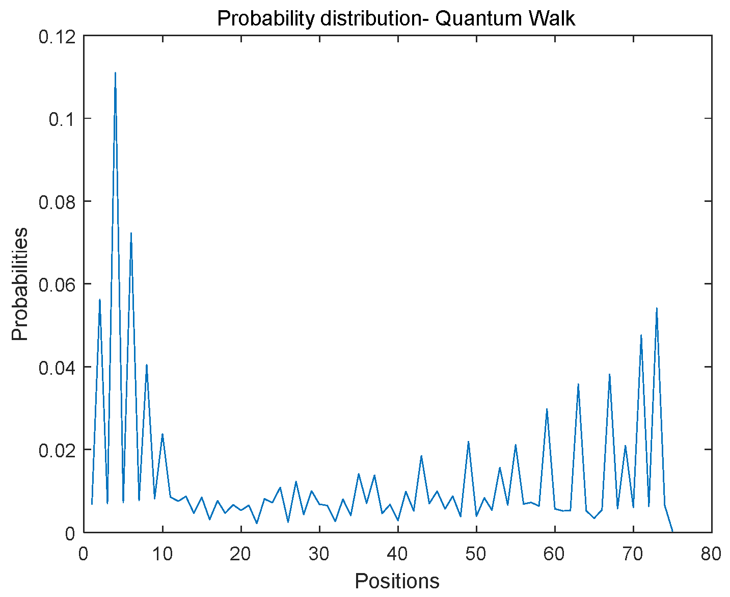
2.1. One-Dimensional Discrete Quantum Walks (1DQWs) on Circles

A one-dimensional discrete quantum walk on a circle [38] whose initial state of the coin operator $O$ is $|o\rangle =\mathsf{\alpha }|0\rangle +\mathsf{\beta }|1\rangle$, where $\alpha$ and $\beta$ are the amplitudes of the initial coin operator which satisfy the normalization equation ${|\alpha |}^2+{|\beta |}^2=1$. During the evolution of the quantum system, the quantum walk is realized by applying the shift operator to the coin operator, which is represented by the global unitary operator $\widehat{M}$, such as in Equation (1):

$$\widehat{M}=\widehat{N}(\widehat{I}\otimes \widehat{O})$$

(1)

where $\widehat{N}$ represents the shift operator, and its expression is Equation (2):

$$\widehat{N}={\displaystyle \sum }_x(|(x+1)mod T,0\rangle \langle x,0|+|(x-1)mod T,1\rangle \langle x,1|)$$

(2)

$\widehat{I}$ represents the identity matrix. $\widehat{O}$ represents the coin operator, and its expression is Equation (3):

$$\widehat{O}=\left(\begin{array}{cc}\cos \theta & \sin \theta \\ \sin \theta & -\cos \theta \end{array}\right)$$

(3)

where $\theta \in \left[0,\frac{\pi }{2}\right]$.

After $t$ steps, the final state of the entire quantum system is Equation (4):

$${|\psi \rangle }_t={(\widehat{M})}^t{|\psi \rangle }_0$$

(4)

After $t$ steps, the probability of finding a walker at position $x$ is Equation (5):

$$P(x,t)={\displaystyle \sum }_{c\in \left\{0,1\right\}}{|\langle x,c|{(\widehat{M})}^t{|\psi \rangle }_0|}^2$$

(5)

The general situation of the probability distribution of one-dimensional discrete quantum walks on a circle (number of nodes 75; ${\mathsf{\theta }}_0=\frac{\mathsf{\pi }}{3}$; step count $k=165$; the initial coin operator is $\mathrm{c}=\frac{1}{\sqrt{2}}\left[\begin{array}{c}1\\ 1\end{array}\right]$) is shown in Figure 1.

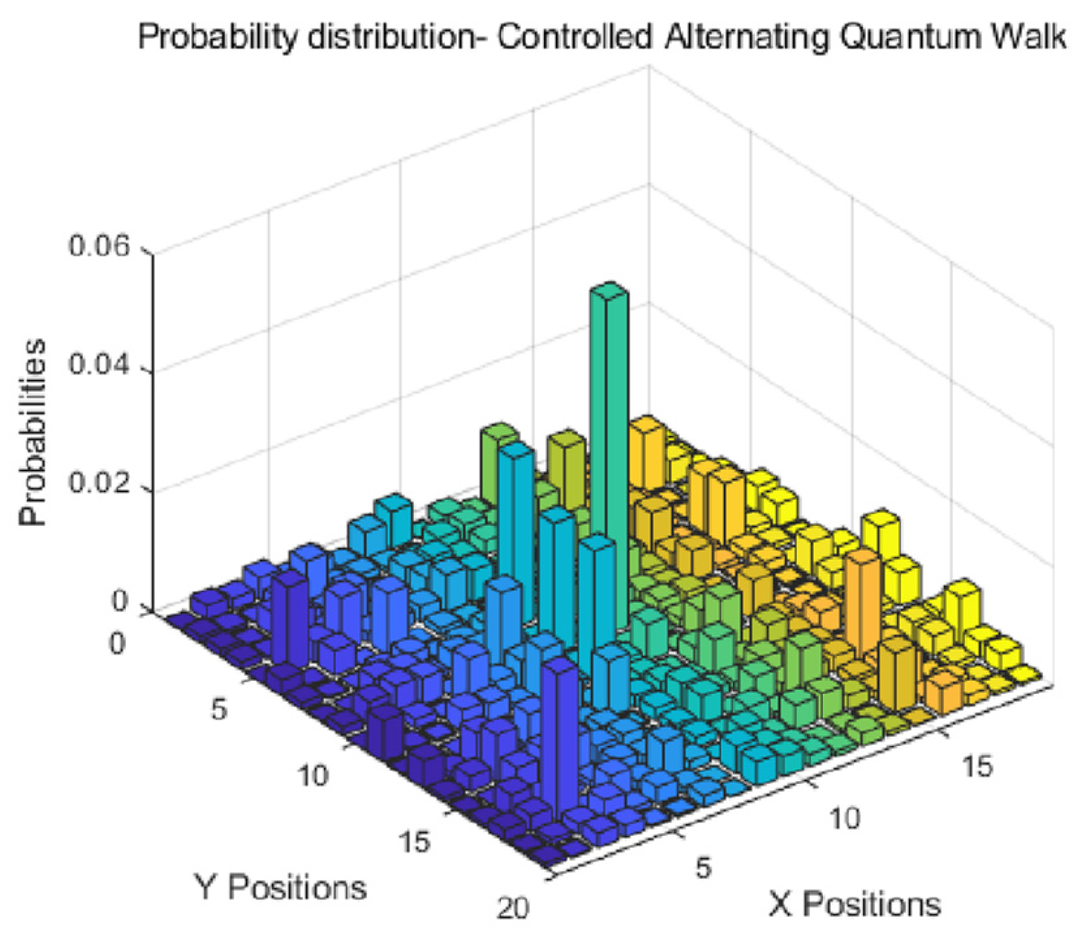
2.2. Controlled Alternate Quantum Walks (CAQWs) on Circles

A controlled alternate quantum walk process on a circle has a string of messages controlling the transform operator at each step [41]. When the $t$-th bit of the message is zero or one, the evolution operator ${\widehat{M}}_0$ or ${\widehat{M}}_1$ is applied to the coin operator, which is expressed as Equations (6) and (7):

$${\widehat{M}}_0={\widehat{N}}_y(\widehat{I}\otimes {\widehat{O}}_0){\widehat{N}}_x(\widehat{I}\otimes {\widehat{O}}_0)$$

(6)

$${\widehat{M}}_1={\widehat{N}}_y(\widehat{I}\otimes {\widehat{O}}_1){\widehat{N}}_x(\widehat{I}\otimes {\widehat{O}}_1)$$

(7)

where ${\widehat{N}}_x$, ${\widehat{N}}_y$ represent the shift operators acting in the $x$ and $y$ directions, respectively, which are expressed as Equations (8) and (9):

$${\widehat{N}}_x={\displaystyle \sum }_{x,y}^T(|(x+1)modT,y,0\rangle \langle x,y,0|+|(x-1)modT,y,1\rangle \langle x,y,1|)$$

(8)

$${\widehat{N}}_y={\displaystyle \sum }_{x,y}^T(|x,(y+1)modT,0\rangle \langle x,y,0|+|x,(y-1)modT,1\rangle \langle x,y,1|)$$

(9)

$\widehat{I}$ represents the identity matrix. ${\widehat{O}}_0$, ${\widehat{O}}_1$ represent two alternating coin operators, whose construction is in the following Equations (10) and (11):

$${\widehat{O}}_0=\left(\begin{array}{cc}\cos {\theta }_0& \sin {\theta }_0\\ \sin {\theta }_0& -\cos {\theta }_0\end{array}\right)$$

(10)

$${\widehat{O}}_1=\left(\begin{array}{cc}\cos {\theta }_1& \sin {\theta }_1\\ \sin {\theta }_1& -\cos {\theta }_1\end{array}\right)$$

(11)

After $t$ steps, the final state of the entire quantum system is Equation (12):

$${|\psi \rangle }_t={(\widehat{M})}^t{|\psi \rangle }_0$$

(12)

After $t$ steps, the magnitude of the probability of finding a walker at position $(x,y)$ is Equation (13). The probability is Equation (14):

$$F(x,y,t)={\displaystyle \sum }_{c\in \left\{0,1\right\}}\langle x,y,c|{(\widehat{M})}^t{|\psi \rangle }_0$$

(13)

$$P(x,y,t)={\displaystyle \sum }_{c\in \left\{0,1\right\}}{|\langle x,y,c|{(\widehat{M})}^t{|\psi \rangle }_0|}^2$$

(14)

The probability distribution of quantum walks controlled by binary message string M on a circle (number of nodes: 19;${\theta }_0=\frac{\pi }{3}$;${\theta }_1=\frac{\pi }{5}$; the initial coin operator is $c=\frac{1}{\sqrt{2}}\left[\begin{array}{c}1\\ 1\end{array}\right]$; $message=\left[01000000111101010101010010100000011110101010101001\right]$), as is shown in Figure 2.

3. Proposed Method

In the following subsections, we describe our proposed encryption algorithm in detail.

3.1. Generate Initial Key

Our key consists of four parts: initial parameters $d_1~d_8$, $sumP$ of plaintext image pixel values, image block size $Bsize$, supplementary parameters $M1$,$N1$, and the number of blocks $Bnum$.

3.1.1. Initial Parameters $d_1~d_8$

We took a plaintext image as the input of SHA-512 and obtained a 128-bit hexadecimal sequence which was divided into 64 groups of sequences $k_1\sim k_{64}$. Each group was an 8-bit byte sequence. According to the 64 groups of sequences, we calculated and generated initial parameters $d_1~d_8$ and use them as keys, such as in Equation (15), the specific steps are as follows:

Step one: Convert $k_1\sim k_{32}$ to binary sequence.

Step two: Convert $k_{33}\sim k_{64}$ into a decimal sequence and take the entire sequence modulo 8 to obtain the cyclic shift bits of the sequence $k_1\sim k_{32}$.

Step three: According to $k_{33}\sim k_{64}$, we need to rotate $k_1\sim k_{32}$, convert it into a decimal sequence, and calculate the initial parameters $d_1~d_8$.

$$\{\begin{array}{c}{d}_1=\frac{k_1\ll mod(k_{33},8)+k_2\ll mod(k_{34},8)+k_3\ll mod(k_{35},8)+k_4\ll mod(k_{36},8)}{4\ast 256+1}\\ d_2=\frac{k_5\ll mod(k_{37},8)+k_6\ll mod(k_{38},8)+k_7\gg mod(k_{39},8)+k_8\gg mod(k_{40},8)}{4\ast 256+1}\\ d_3=\frac{k_9\gg mod(k_{41},8)+k_{10}\gg mod(k_{42},8)+k_{11}\gg mod(k_{43},8)+k_{12}\gg mod(k_{44},8)}{4\ast 256+1}\\ d_4=\frac{k_{13}\ll mod(k_{45},8)\oplus k_{14}\ll mod(k_{46},8)\oplus k_{15}\ll mod(k_{47},8)\oplus k_{16}\ll mod(k_{48},8)}{256+1}\\ d_5=\frac{k_{17}\gg mod(k_{49},8)\oplus k_{18}\gg mod(k_{50},8)\oplus k_{19}\gg mod(k_{51},8)\oplus k_{20}\gg mod(k_{52},8)}{256+1}\\ d_6=\frac{k_{21}\gg mod(k_{53},8)+k_{22}\ll mod(k_{54},8)\oplus k_{23}\ll mod(k_{55},8)\oplus k_{24}\ll mod(k_{56},8)}{2\ast 256+1}\\ d_7=\frac{k_{25}\gg mod(k_{57},8)\oplus k_{26}\gg mod(k_{58},8)\oplus k_{27}\gg mod(k_{59},8)+k_{28}\ll mod(k_{60},8)}{2\ast 256+1}\\ d_8=\frac{k_{29}\gg mod(k_{61},8)\oplus k_{30}\gg mod(k_{62},8)+k_{31}\ll mod(k_{63},8)\oplus k_{32}\ll mod(k_{64},8)}{2\ast 256+1}\end{array}$$

(15)

where $\ll$ represents a cyclic left shift to the binary sequence, $\gg$ represents a cyclic right shift to a binary sequence, and $\oplus$ represents the exclusive-or operator.

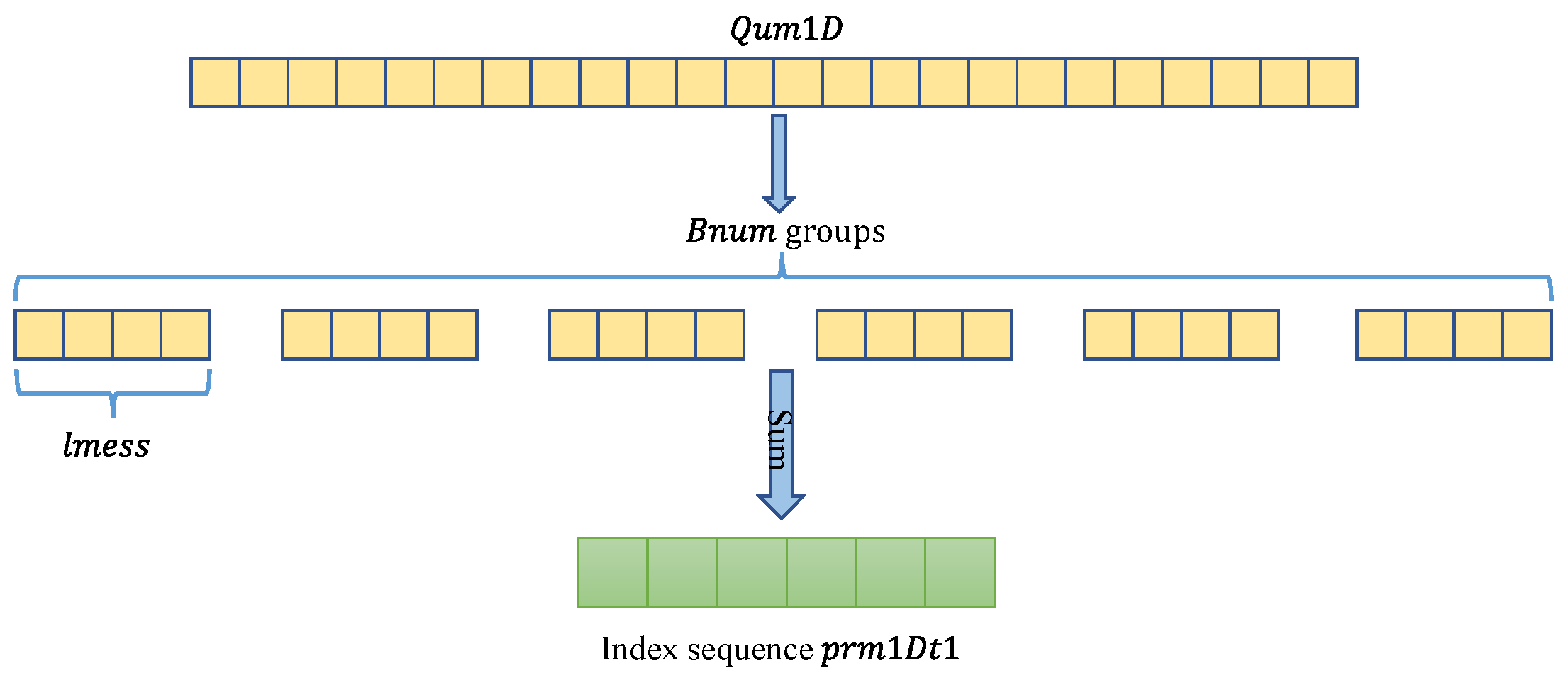
3.1.2. Sum of Plaintext Image Pixel Values $sumP$

Accumulate and sum all pixel values of the plaintext image to obtain the key $sumP$, whose expression is Equation (16):

$$sumP={\displaystyle \sum }_{x=1}^m{\displaystyle \sum }_{y=1}^{n}P(x,y)$$

(16)

where $P(x,y)$ represents the pixel value at the $(x,y)$ position.

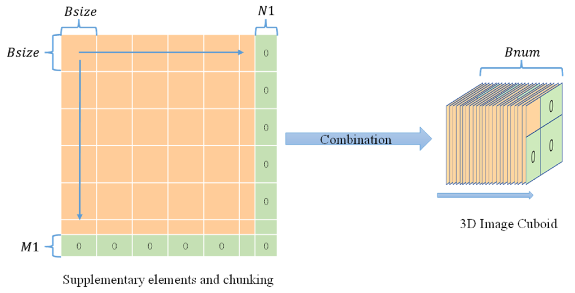
3.1.3. Image block size $Bsize$

First, select the short side of the image, and assume $M$ is the short side. Then, divide $M$ by an odd number within 11$~$30, and select the odd number corresponding to the number with the largest fractional part from the result as the block size $Bsize$.

3.1.4. Supplementary Parameters $M1$, $N1$ and Number of Blocks $Bnum$

According to the block size $Bsize$, the rows and columns of the image are filled with numbers that are divisible by $Bsize$, and the number of rows $M1$ and the number of columns $N1$ of the supplementary element 0 are used as the key. The calculation formula is Equation (17):

$$M1=mod(M,Bsize);N1=mod(N,Bsize)$$

(17)

where $mod$ represents the modulo, $M$ and $N$ are the number of rows and columns of the original image, and $Bsize$ is the block size.

After adding elements to the original image, its row and column are $M2 and N2$, and the number of blocks is calculated by the following Equation (18):

$$Bnum=\frac{M2}{Bsize}\ast \frac{N2}{Bsize}$$

(18)

3.2. Generating 3D Probability Magnitude Matrix, 3D Probability Distribution Matrix, and 3D Quantum Hash Sequence by Using Quantum Walks

We used a one-dimensional quantum walk to generate a one-dimensional probability distribution sequence, then encoded the probability distribution sequence to generate a quaternary message and performed controlled alternating quantum walks by encoding the message. Finally, it generated the probability amplitude matrix and probability distribution matrix of multiple CAQWs by combining a 3D probability amplitude matrix and 3D probability distribution matrix and then generated a 3D quantum hash sequence according to the probability distribution matrix. We applied the generated one-dimensional probability distribution sequence, 3D probability amplitude matrix, 3D probability distribution matrix, and 3D quantum hash sequence to the three-dimensional cuboid image encryption algorithm.

3.2.1. Generation of Initial Parameters for 1DQWs

(1)

Number of nodes on the circle

According to the key $sumP$ generated in Section 3.1.2, the ten-digit number $SP$ of the sum of pixel values is calculated by Equation (19). Then calculate the length $lmess$ of the message through the parameter $d_1$ in Section 3.1.1, as shown in Equation (20). If $sumP=0$, then the length of the message $lmess1$ is Equation (21). Finally, the number of nodes $TC$ of the circle is given by Equation (22).

$$SP=floor({log}_{10}sumP)$$

(19)

$$lmess=mod(floor(sumP\ast d_1\ast {10}^{15-SP}),2^5)+1+Bsize$$

(20)

$$lmess1=13+Bsize$$

(21)

$$TC=lmess1\ast Bnum$$

(22)

where $floor$ means rounding down, $lo{g}_{10}$ is a logarithmic function with base 10, and $mod$ means a modulo operation.

(2)

Coin parameter $\theta$

The coin parameter $\theta$ is calculated by the parameter $d_2$ of Section 3.1.1, as shown in Equation (23).

$$\theta =mod(d_2\ast {10}^{15}\ast (\frac{\pi }{7}+2),\frac{\pi }{2})$$

(23)

where $mod$ represents the modulo operation.

(3)

The initial state of the coin

The initial state of the coin is $\alpha |0\rangle +\beta |1\rangle$. We used the parameters $d_3$ and $d_4$ in Section 3.1.1 to generate the initial state of the coin $\alpha ,\beta$, $\alpha ,\beta$ is expressed as the following Equation (14). Because the coin operator needs to satisfy ${|\alpha |}^2+{|\beta |}^2=1$, we constructed the quadratic equation of one variable of Equation (25) to calculate the initial state of the generated coins.

$$\mathsf{\alpha }=d_3+(\frac{d_3}{2})i;\mathsf{\beta }=(\frac{d_4}{2})+xi$$

(24)

$$f=1-{\left(\sqrt{d_3^2+{(\frac{d_3}{2})}^2}\right)}^2-{\left(\sqrt{{(\frac{d_4}{2})}^2+x^2}\right)}^2=0$$

(25)

where $\alpha ,\beta$ are the amplitude and phase of the initial state (complex number), $i$ represents the complex unit, $f$ represents the quadratic equation to be solved, and $x$ represents the unknown parameter.

3.2.2. Generation of Initial Parameters of CAQWs

(1)

The number of nodes on the circle of CAQWs is equal to the block size $Bsize$.

(2)

Coin parameters ${\theta }_0,{\theta }_1$

The coin parameters ${\theta }_0,{\theta }_1$ are calculated by the parameters $d_7$ and $d_8$ in Section 3.1.1, as shown in Equations (26) and (27)

$${\theta }_0=mod(d_7\ast {10}^{15}+(\frac{\pi }{5}+2),\frac{\pi }{2})$$

(26)

$${\theta }_1=mod(d_8\ast {10}^{15}+(\frac{\pi }{5}+0.1),\frac{\pi }{2})$$

(27)

(3)

Initial state of the coin

Similar to the initial state of the coin of 1DQWs, the expressions of $\alpha 1,\beta 1$ are Equation (28). Because the coin operator needs to satisfy ${|\alpha 1|}^2+{|\beta 1|}^2=1$, we constructed the quadratic equation of one variable of Equation (29) to calculate the initial state of the generated coins.

$$\alpha 1=(\frac{d_5}{2})+(\frac{d_5}{3})i;\beta 1=(\frac{d_6}{2})+x1i$$

(28)

$$f1=1-{\left(\sqrt{{(\frac{d_5}{2})}^2+{(\frac{d_5}{3})}^2}\right)}^2-{\left(\sqrt{{(\frac{d_6}{2})}^2+x{1}^2}\right)}^2=0$$

(29)

where $\alpha 1,\beta 1$ are the amplitude and phase of the initial state (complex number), $i$ represents the complex unit. $f1$ represents the quadratic equation to be solved, and $x1$ represents the unknown parameter.

3.2.3. Generating Probability Distribution Sequences Using 1DQWs

According to the initial parameters, we performed a 1D discrete quantum walk [38]. After $t$ steps, the probability of finding a walker at position $x$ is Equation (30), and we denoted this sequence of probability distributions as $Qum1D$.

$$P(x,t)={\displaystyle \sum }_{c\in \left\{0,1\right\}}{|\langle x,c|{(\widehat{M})}^t{|\psi \rangle }_0|}^2$$

(30)

where $P(x,t)$ represents the probability of finding a walker at $x$ after $t$ steps.

3.2.4. Message Encoding

We mapped the probability distribution sequence $Qum1D$ generated by 1DQWs to values 0–255, as shown in Equation (31), and quaternary encoded it and the encoded $message$ as the message.

$$message=mod(mod(floor(Qum1D\ast {10}^{200}),256),4)$$

(31)

where $mod$ represents the modulo operation, and $floor$ represents the rounding down.

3.2.5. Controlled Alternate Quantum Walks for Message Encoding

In the proposed image encryption algorithm, we improved the two-dimensional controlled alternating walk model and encoded the sequence generated by 1DQWs into a quaternary sequence as a control message. We also applied the quaternary message encoding to the evolution process of the quantum system [40] by using Equation (32) to represent the global unitary operators ${\widehat{M}}_0$, ${\widehat{M}}_1$, ${\widehat{M}}_2$, ${\widehat{M}}_3$.

$$\{\begin{array}{c}{\widehat{M}}_0={\widehat{N}}_y(\widehat{I}\otimes {\widehat{O}}_0){\widehat{N}}_x(\widehat{I}\otimes {\widehat{O}}_0)\\ {\widehat{M}}_1={\widehat{N}}_y(\widehat{I}\otimes {\widehat{O}}_0){\widehat{N}}_x(\widehat{I}\otimes {\widehat{O}}_1)\\ {\widehat{M}}_2={\widehat{N}}_y(\widehat{I}\otimes {\widehat{O}}_1){\widehat{N}}_x(\widehat{I}\otimes {\widehat{O}}_0)\\ {\widehat{M}}_3={\widehat{N}}_y(\widehat{I}\otimes {\widehat{O}}_1){\widehat{N}}_x(\widehat{I}\otimes {\widehat{O}}_1)\end{array}$$

(32)

Assuming that the message string generated by 1DQWs is “320102”, the state of the entire system can be expressed as Equation (33):

$${|\psi \rangle }_6={\widehat{M}}_2{\widehat{M}}_0{\widehat{M}}_1{\widehat{M}}_0{\widehat{M}}_2{\widehat{M}}_3{|\psi \rangle }_0$$

(33)

After $t$ steps, the final state of the entire quantum system is Equation (34):

$${|\psi \rangle }_t={(\widehat{M})}^t{|\psi \rangle }_0$$

(34)

After $t$ steps, the probability amplitude of finding a walker at position $(x,y)$ is Equation (35), and the probability is Equation (36):

$$F(x,y,t)={\displaystyle \sum }_{c\in \left\{0,1\right\}}\langle x,y,c|{(\widehat{M})}^t{|\psi \rangle }_0$$

(35)

$$P(x,y,t)={\displaystyle \sum }_{c\in \left\{0,1\right\}}{|\langle x,y,c|{(\widehat{M})}^t{|\psi \rangle }_0|}^2$$

(36)

3.2.6. Three-Dimensional Probability Amplitude Matrix and Three-Dimensional Probability Distribution Matrix

According to the number of blocks $Bnum$ in Section 3.1.4, we divided the message encoding $message$ into $Bnum$ groups and used Section 3.2.2 to calculate the generated initial parameters of the system. According to the corresponding message encoding, we performed $Bnum$ times of message encoding-controlled alternate quantum walks on the circle and finally generated a 3D probability amplitude matrix $fre$ of size $2\ast (Bsize\ast Bsize)\ast Bnum$, whose expression is Equation (37). At the same time, a 3D probability distribution matrix $Qum2D$ of size $Bsize\ast Bsize\ast Bnum$ was generated, and its expression is Equation (38).

$$fre(2,Bsize\ast Bsize,i)=\phi (F(x,y,t),message(i))i=1,\dots ,Bnum$$

(37)

where $\phi (F(x,y,t),message(i))$ represents the probability amplitude matrix which generated under the control of the $i-th$ group of $message$ encoding messages.

$$Qum2D(Bsize,Bsize,i)=\omega (P(x,y,t),message(i))i=1,\dots ,Bnum$$

(38)

where $\omega (P(x,y,t),message(i))$ represents the probability matrix which generated under the control of the $i-th$ group of $message$ encoding messages.

3.2.7. Three-Dimensional Quantum Hash Sequence

Quantum hash sequences have chaotic-dynamics-like properties and can be used to generate pseudorandom numbers. We converted the 3D probability distribution matrix $Qum2D$, which was generated in Section 3.2.6, into a binary string using Equations (39) and (40) and finally obtained the 3D quantum hash sequence $Btest$. In the diffusion stage, we used the 3D quantum hash sequence $Btest$ to complete the diffusion operation.

$$B=mod(floor(Qum2D\ast {10}^{15}),256)$$

(39)

$$Btest=dec2bin(B)$$

(40)

where $dec2bin$ means converting a decimal number to binary.

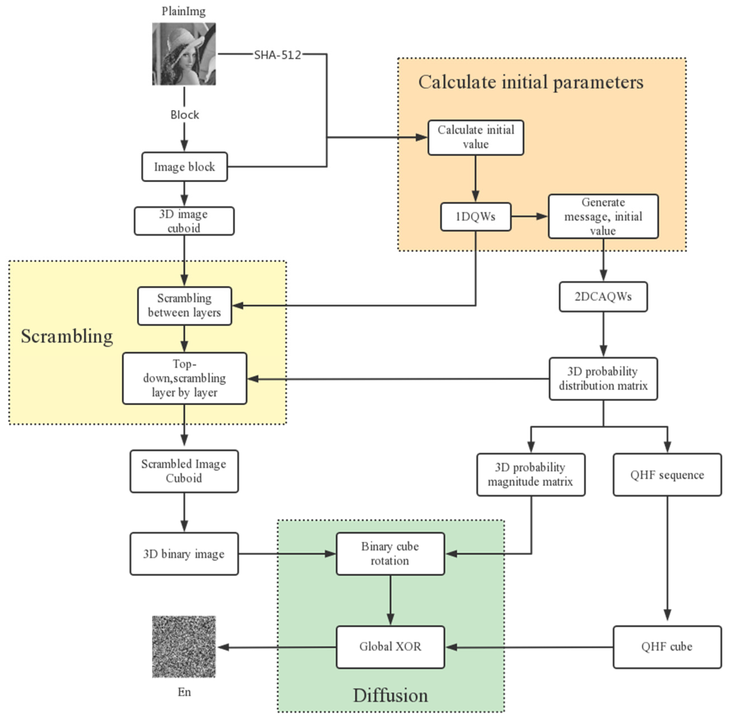
3.3. Image Encryption Process

Combining the discrete quantum walk model, we propose a three-dimensional cuboid image encryption algorithm with two rounds of scrambling and two rounds of diffusion operations. First, we used 1DQWs to generate a probability value sequence $Qum1D$, then encoded $Qum1D$ into a quaternary message $message$. Then, we used the encoded message to control the alternate quantum walk model to generate a 3D probability amplitude matrix and 3D probability distribution matrix. Finally, we used the 3D probability distribution matrix obtain the 3D quantum hash series. The operation is shown in Algorithm 1. We used the probability value sequence $Qum1D$ and 3D probability distribution matrix to complete the image scrambling and used the 3D probability magnitude matrix and 3D quantum hash series to diffuse the image to obtain the final encrypted image. The operation is shown in Algorithm 2. The following are the specific steps of our proposed encryption scheme, and its flow chart is shown in Figure 3.

Algorithm 1. Sequence generation.

Input: Original image(PlainImg) Output$: d_1~d_8, Qum1D, message, fre, Qum2D, Btest$ 1 $k_1\sim k_{64}\leftarrow$SHA-512(PlainImg) 2 $d_1~d_8\leftarrow$Generate initial key parameters based on $k_1\sim k_{64}$ 3 Calculation of 1DQWs and 2DCAQWs 4 $Qum1D\leftarrow 1DQWs$($TC,t,\theta ,\alpha ,\beta$) // 1DQWs on a circle with node number $TC$ 5 $message\leftarrow encoding(Qum1D)$ // Quadratic encoding 6 $fre(2,Bsize\ast Bsize,i)\leftarrow \phi (F(x,y,t),message(i))i=1,\dots ,Bnum;$ 7 $Qum2D(Bsize,Bsize,i)\leftarrow \omega (P(x,y,t),message(i))i=1,\dots ,Bnum$ // Alternating quantum walks with $Bnum$ sub-message encoding control on a circle 8 $Btest\leftarrow dec2bin(Qum2D)$ // Complete diffusion operation using 3D quantum hash sequence Btest

Algorithm 2. Encryption algorithms.

Input: Original image(PlainImg), $Qum1D$, $message$, $fre$, $Qum2D$, $Btest$ Output: Encrypted images($En$) 1 Image block ($Bsize\ast Bsize\ast Bnum)\leftarrow$chunking the image 2 $Plain3D\leftarrow$Integrating image blocks as rectangles 3 $prm1Dt\leftarrow sum(reshape(Qum1D,lmess,Bnum))$; //Group summation 4 $\left[~,prm1Dindex\right]\leftarrow sort(prm1Dt)$ // Sort 5 $PrmP3D\leftarrow$ Displacement between layers according to its index sequence $prm1Dindex$ for the image rectangle $Plain3D$ 6 $Prm2\leftarrow$ Sorting and dislocation inside each depth layer using $Qum2D$ 7 for j $\leftarrow$ 1 to B_num 8  $\mathrm{BinP}3=\mathrm{dec}2\mathrm{bin}(Prm2$); 9  for i$\leftarrow$1 to x ∗ y do 10    $\mathrm{BinP}3\_\mathrm{t}\leftarrow$reshape$(\mathrm{BinP}3)$ 11    If A > B 12     Bin_P3$\leftarrow$$\mathrm{rot}90(\mathrm{BinP}3\_\mathrm{t}$ Upper)// Upper layer rotated 90 degrees counterclockwise 13    else 14     Bin_P3$\leftarrow$$\mathrm{rot}90(\mathrm{BinP}3\_\mathrm{t}$ Lower) //Lower layer rotated clockwise by 90 degrees 15    end 16    P3bin(i,:) = reshape(Bin_P3); 17   end 18   P3bin1 = bin2dec(P3bin); 19   P3bin2 = reshape(P3bin1, x, y); 20 end 21 $Ctest=bitxor(Btest,P3bin2)$ // Global xor 22 $En\leftarrow$Tiling the image block $Ctest$

3.3.1. Generation of Image Cuboid

Step one: Image segmentation

According to the supplementary parameters $M1$ and $N1$ generated in Section 3.1.4, the plaintext image blocks were supplemented with zero elements in row $M1$ and column $N1$, and then according to the image block size $Bsize$ generated in Section 3.1.3 and the number of blocks $Bnum$ generated in Section 3.1.4, we divided the filled image into image blocks whose size is $Bsize\ast Bsize$, $Bnum$ number.

Step two: Combine into a 3D image cuboid

The $Bnum$ image blocks generated by Step One were converted into a three-dimensional image cuboid $plain3D$ with the size of $Bsize\ast Bsize\ast Bnum$, line by line, from left to right, and from top to bottom, as shown in Figure 4.

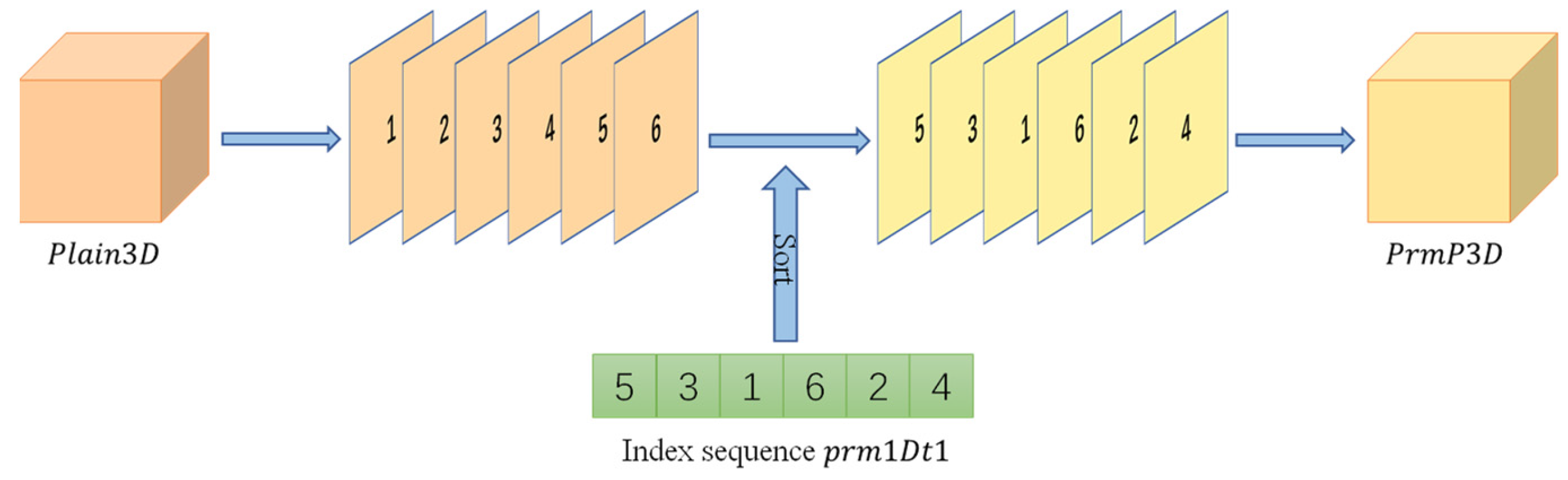
3.3.2. Two Rounds of Scrambling

Step one: Interlayer scrambling based on one-dimensional quantum walk.

According to Equation (41), we divided the probability distribution sequence $Qum1D$ generated in Section 3.2.3 into $Bnum$ groups and then summed the sequences of each group to obtain the sequence $prm1Dt$. The operation process is shown in Figure 5.

Then, Equation (42) was used to sort $prm1Dt$ from small to large, and the image cuboid $Plain3D$ was scrambled between layers according to its index sequence $prm1Dindex$ to obtain the scrambled image block $PrmP3D$ between layers, as shown in Figure 6.

$$prm1Dt=sum(reshape(Qum1D,lmess,Bnum))$$

(41)

where $reshape$ is an array reconstruction function, $lmess$ represents the message length, $Bnum$ represents the number of blocks, and $sum$ represents the sum of the array by columns.

$$\left[~,prm1Dindex\right]=sort(prm1Dt)$$

(42)

where $sort$ is the sorting function and $prm1Dindex$ is the sequence of index sorting.

Step Two: Layer-by-layer scrambling based on 3D probability distribution matrix

The three-dimensional probability distribution matrix $Qum2D$ generated in Section 3.2.6 sorted the image block from smallest to largest in order from top to bottom in each depth layer and used the index sort matrix generated at each layer. The image block $PrmP3D$ was scrambled layer by layer to obtain a new image block $Prm2$, as shown in Figure 7.

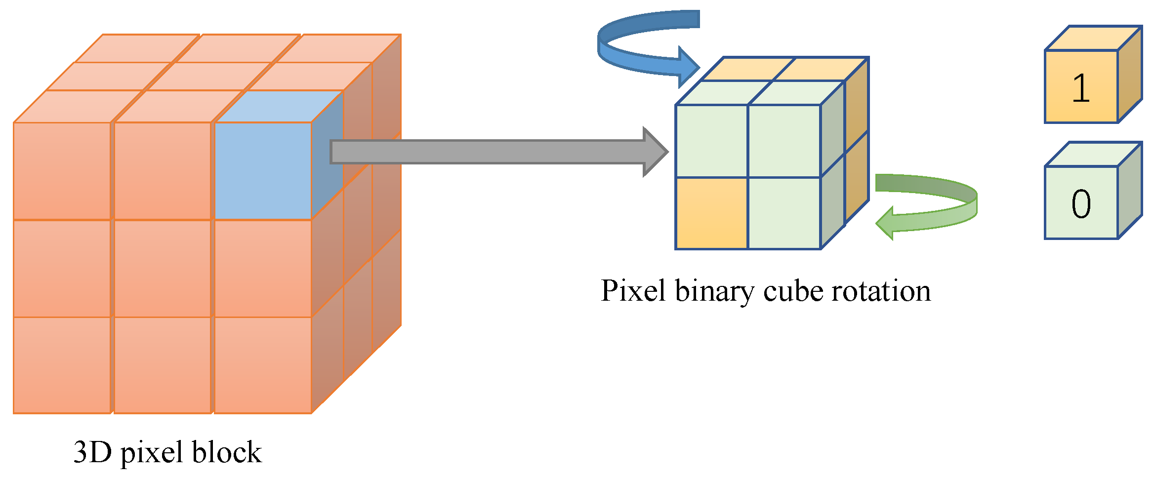
3.3.3. Two Rounds of Diffusion

Step one: Binary cube rotation based on probability magnitude matrix

As shown in Figure 8, each 0–255 pixel value of the image block $Prm2$ obtained by scrambling in Section 3.3.2 was operated from left to right, layer by layer. Then, we operated it from back to front and top to bottom and encoded as a binary cube. According to the 3D probability amplitude matrix obtained in Section 3.2.6, the binary cube was rotated. We divided the probability amplitude into A direction and B direction. If A > B, the upper layer of the binary cube was rotated 90 degrees counterclockwise; otherwise, the lower layer of the binary cube was rotated 90 degrees clockwise. Finally, the binary cube corresponding to each pixel value was converted into a binary sequence, and we obtained the 3D image block $P3bin$ after the binary cube rotation operation.

Step two: Diffusion based on 3D quantum hash sequence

By using the 3D quantum hash series $Btest$ obtained in Section 3.2.7, we performed a global bitwise XOR operation with the 3D image block $P3bin$ according to Equation (43). We converted it into a decimal sequence and obtained the image block $Ctest$. Then, we tiled the image block $Ctest$ to obtain the final encrypted image $En$.

$$Ctest=bitxor(Btest,P3bin)$$

(43)

where $bitxor$ means bitwise exclusive or.

3.4. Image Decryption Process

The image decryption process is the reverse operation of the encryption process, and the steps are as follows:

Step one: According to the key $Bsize$ in Section 3.1.3 and the key $Bnum$ in Section 3.1.4, we divided the encrypted image $En$ into blocks and then combined them into cubes $De3D$.

Step two: We converted each pixel value of the cube $De3D$ into a binary sequence and performed a global bitwise XOR operation with the 3D quantum hash series $Btest$ which was obtained in Section 3.2.7 to acquire the image block $De1$.

Step three: Each pixel value of image block $De1$ was encoded into a binary cub, and a reverse rotation operation was performed on the binary cube according to the three-dimensional probability amplitude matrix obtained in Section 3.2.6. This operation is a reverse of Section 3.3.3, resulting in an image block $De2$.

Step four: The 3D probability distribution matrix $Qum2D$ generated in Section 3.2.6 was sorted by index for each layer, in the order from the top to the bottom. The image block $De2$ was inversely indexed and scrambled layer by layer according to the index order to obtain $De3$.

Step five: According to the index $prm1Dindex$ generated in Section 3.3.2, $De3$ was scrambled with interlayer inverse index to obtain $De4$.

Step six: By tiling the image block $De4$ obtained in the previous step and removing the supplementary zero elements by row and column according to the keys $M1$ and $N1$ obtained in Section 3.1.4, we obtained the final decrypted image $De$.

4. Simulation Results and Security Analysis

In order to test the security performance of the proposed image encryption scheme, we used MATLAB R2020b software to conduct simulation experiments on a computer with Windows 10 system, 16 GB memory, and i5-10500 CPU. The images we used in testing included 256 ∗ 256 square images (Lena, Baboon, Peppers, White, Black), 512 ∗ 512 square images (Barbara, Cameraman, Livingroom), irregular Lena image, and images from standard 25 grayscale images of the USC-SIPI image database.

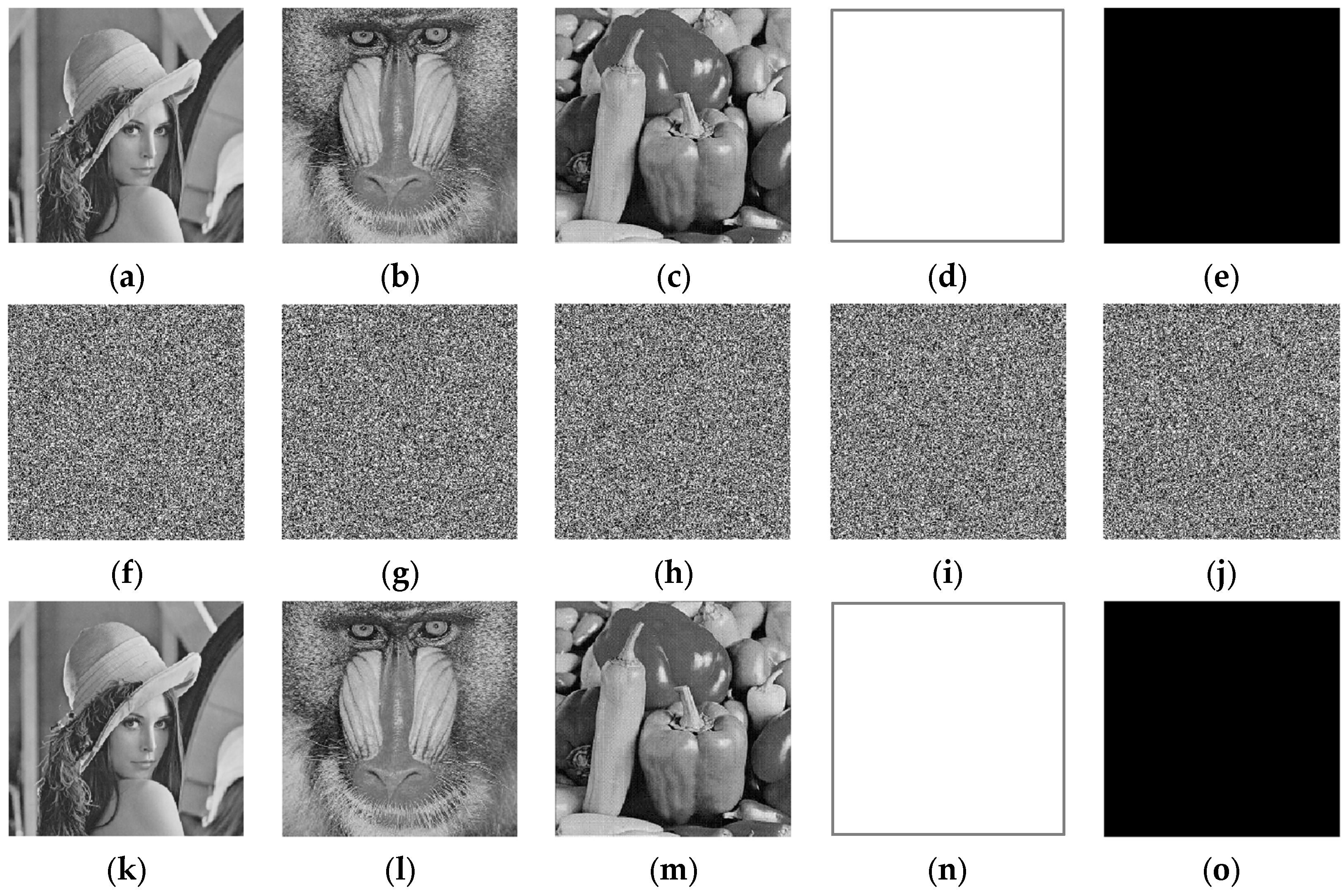
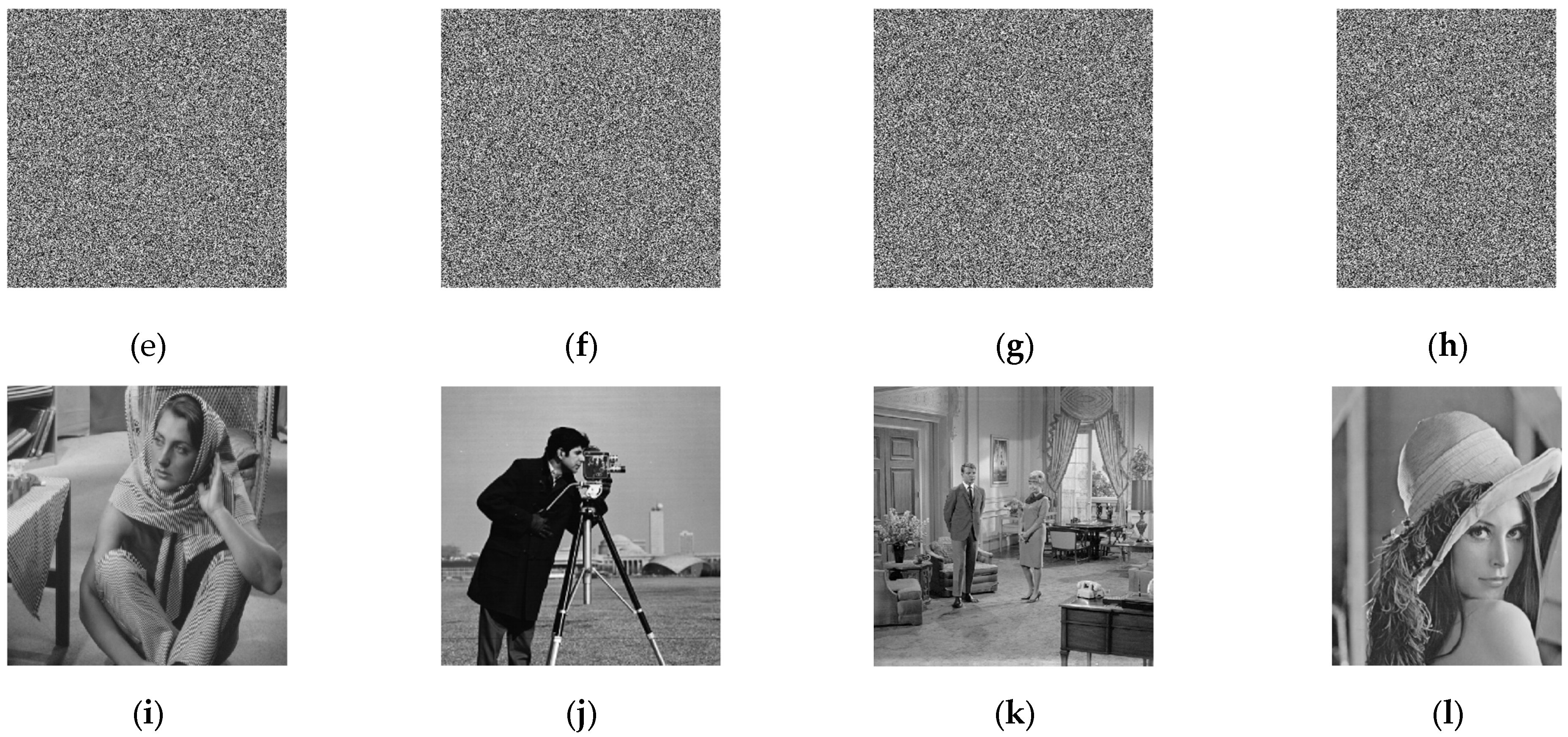
4.1. Encryption and Decryption Results

In this paper, 256 ∗ 256, 512 ∗ 512 square images and irregular Lena image were used for testing. The test results of 256 ∗ 256 images (Lena, Baboon, Peppers, White, Black) are shown in Figure 9. The encryption and decryption results of 512 ∗ 512 images (Barbara, Cameraman, Livingroom) and irregular Lena images are shown in Figure 10. The encrypted images shown in the figure cannot show any meaningful information, and the original images with rich information can be obtained by decrypting with the correct key.

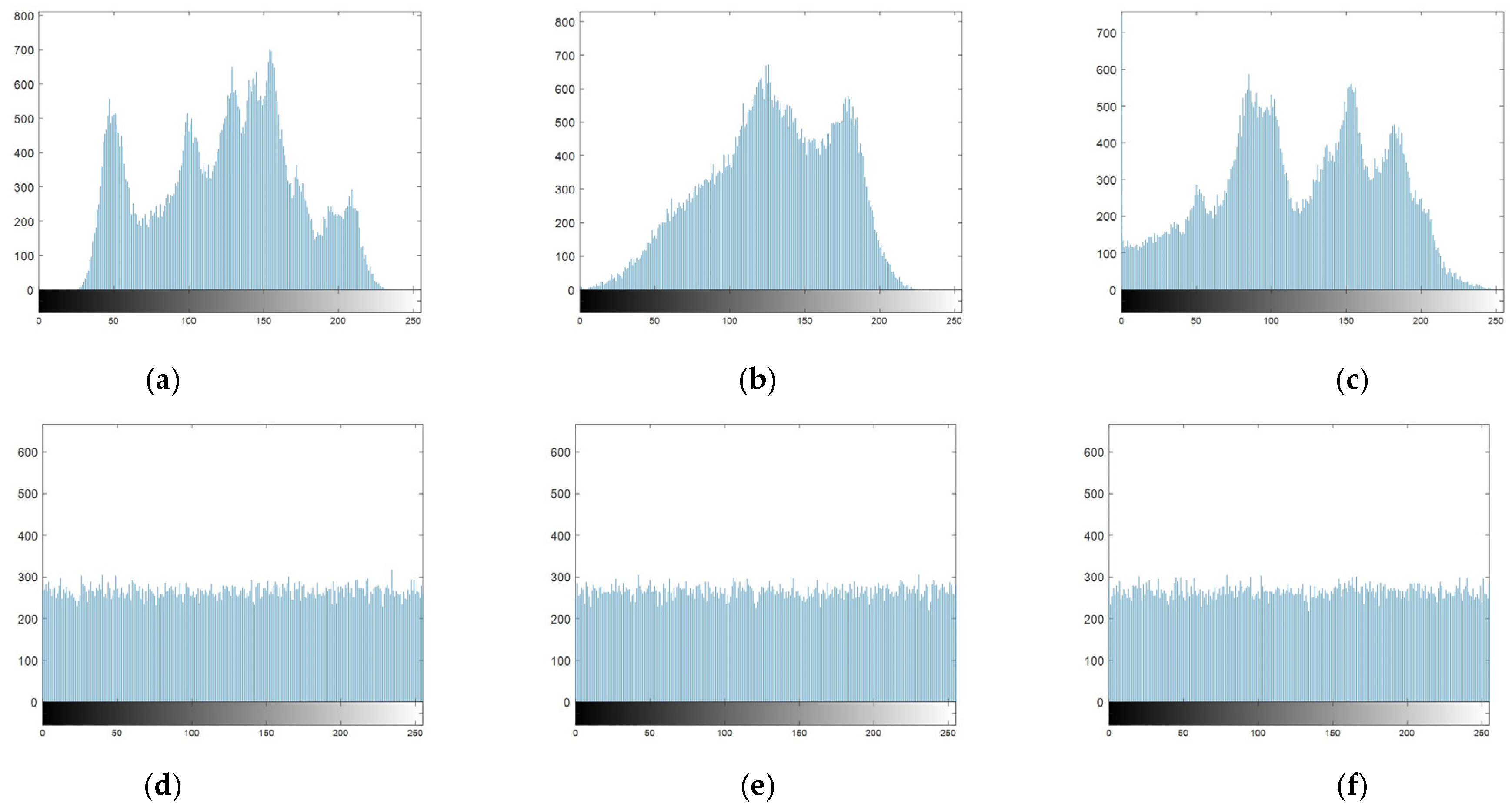
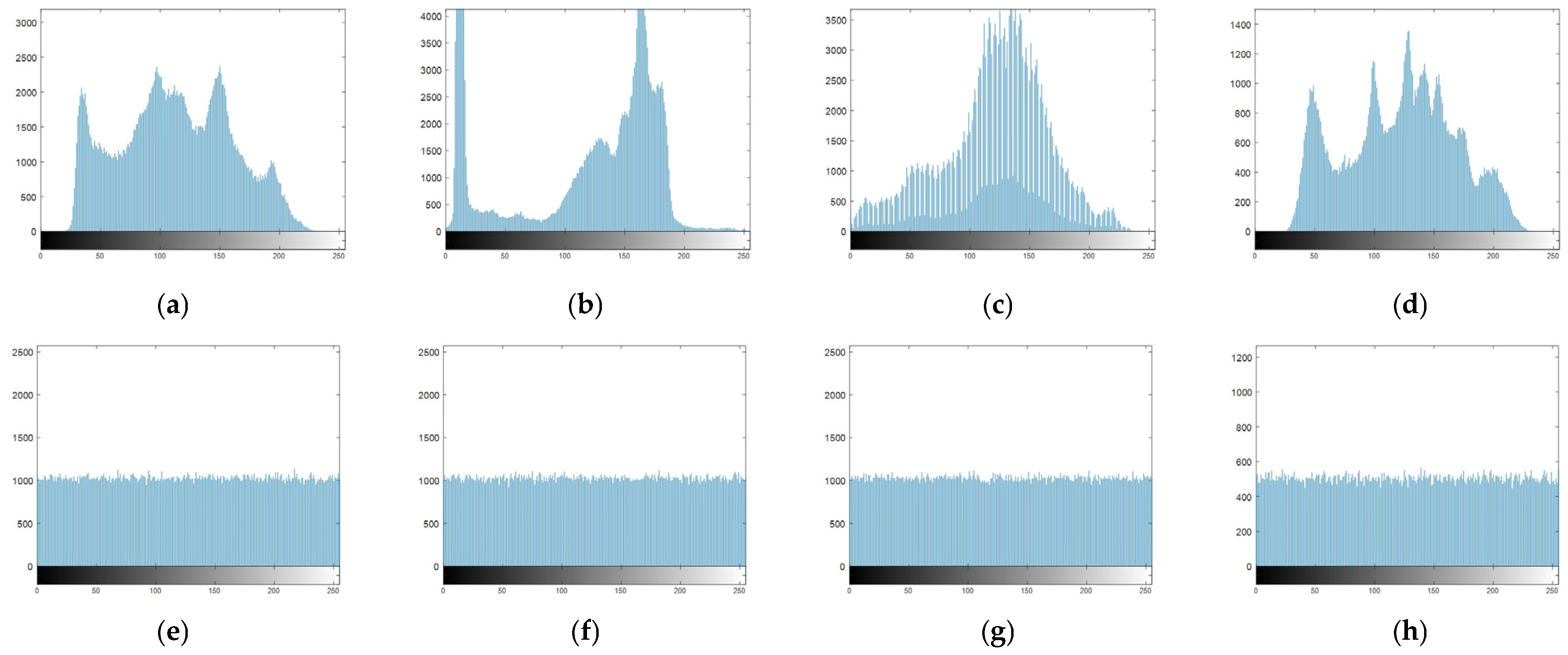
4.2. Histogram Analysis

The pixel histogram shows the distribution of different pixel values in the image. We tested and analyzed the histogram of encrypted images. The histogram analysis results of 256 ∗ 256 size images are shown in Figure 11, and the histogram analysis results of 512 ∗ 512 size images and irregular Lena image are shown in Figure 12. It can be seen that the distribution frequency of pixel values in the encrypted images is relatively uniform, and the trend of the histogram is stable, which has a good ability to resist statistical attacks.

4.3. ${\chi }^2$ Test

We use the ${\chi }^2$ test to describe the distribution of the pixel histogram [42], whose formula is Equation (44):

$${\chi }^2={\displaystyle \sum }_{i=1}^{255}\frac{{(v_i-v_0)}^2}{v_0}$$

(44)

where ${\chi }^2$ represents the value of the chi-square test, $i$ represents the pixel value, $v_i$ represents the frequency of the pixel value $i$ in the image, and $v_0$ represents the expected frequency of the pixel value $i$, $v_0=(M\ast N)/256$. The smaller the value of the ${\chi }^2$ test, the more uniform the pixel distribution. When the confidence is $\alpha =0.05$, the condition for passing the test is that ${\chi }^2$ is less than $293.24783$.

Table 1. ${\chi }^2$ test (256 ∗ 256).

Image	Lena	Baboon	Peppers	White	Black	Avg.	Ref. [9]	Ref. [33]
Plaintext	39,868.727	44,739.305	26,311.578	16,711,680	16,711,680	-	-	-
Ciphertext	219.269	216.589	225.765	259.881	241.390	232.579	244.159	254.078

(Lena, Baboon, Peppers, White, Black) and

Table 2. ${\chi }^2$ test (512 ∗ 512 and irregular).

Image	Barbara	Cameraman	Livingroom	Irregular Lena	Avg.	Ref. [18]
Plaintext	14,4101.119	418,530.147	276,815.883	74,075.357	-	-
Ciphertext	238.454	250.778	245.376	250.828	246.359	260.400

(Barbara, Cameraman, Livingroom, Irregular Lena) show the test results of plaintext images and the results in comparison with others’ methods. The images were encrypted with different sizes, and all results passed the test conditions, which shows that our algorithm has a good ability to resist statistical attacks.

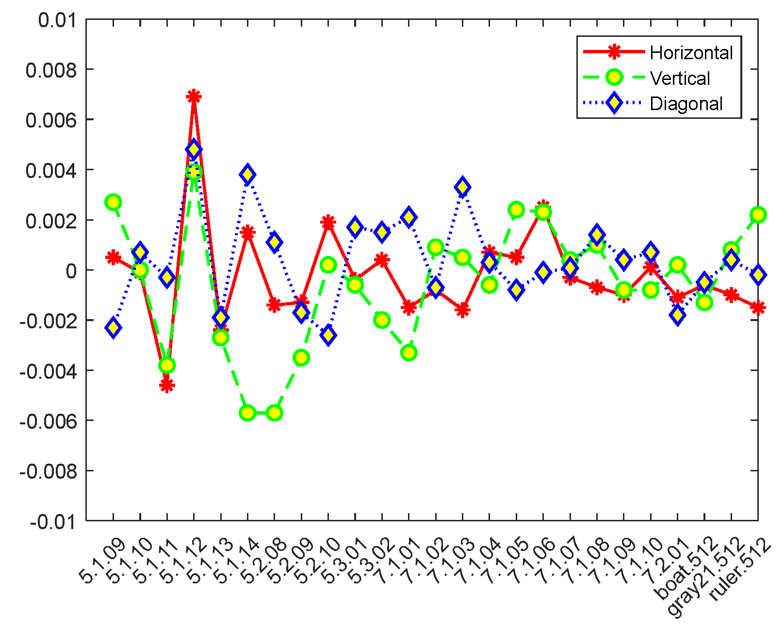
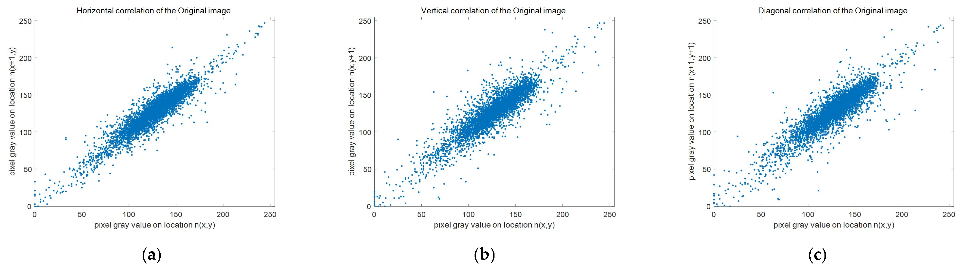
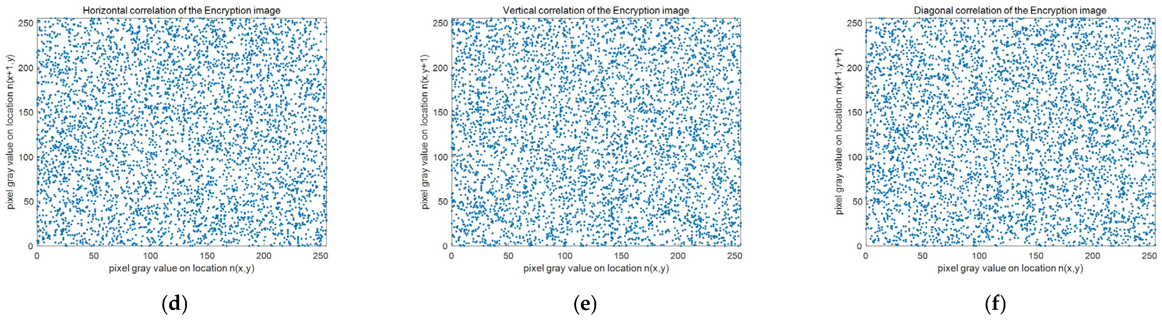
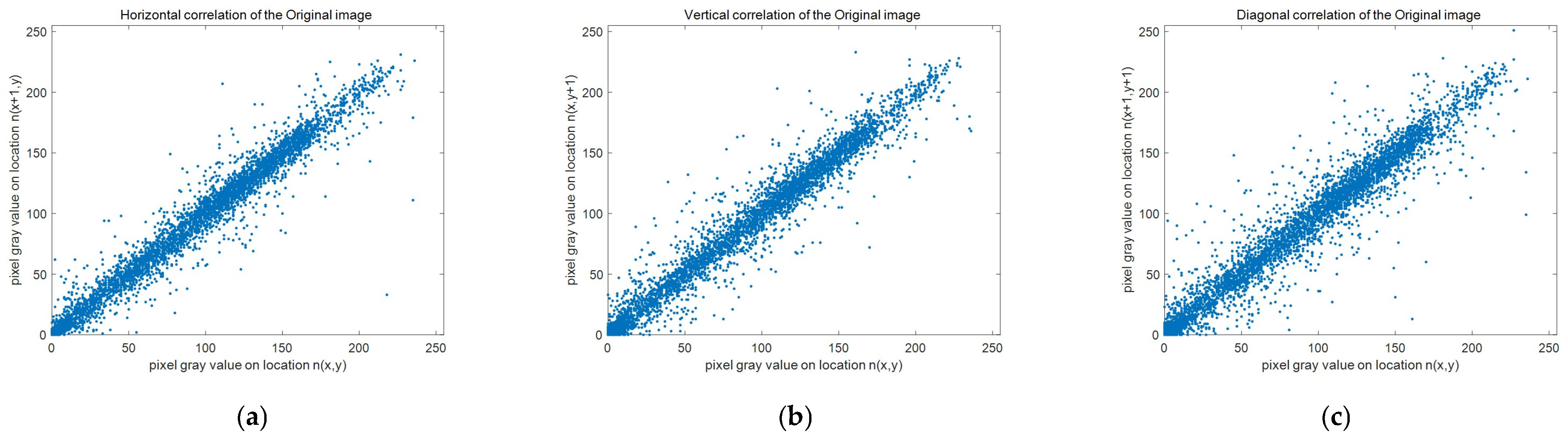
4.4. Correlation Coefficient Analysis

There is a strong correlation between the adjacent pixels of the original image, and the lower the correlation of the ciphertext image, the stronger the resistance of the algorithm to statistical attacks. The calculation formula of pixel correlation is such as Equations (45)–(47):

$$r_{xy}=\frac{E((x-E(x))(y-E(y)))}{\sqrt{D(x)D(y)}}$$

(45)

$$E(x)=\frac{1}{N}{\displaystyle \sum }_{i=1}^N{x}_i$$

(46)

$$D(x)=\frac{{{\displaystyle \sum }}_{i=1}^n{(x_i-E(x))}^2}{N}$$

(47)

where $r_{xy}$ is the pixel correlation coefficient, and $E(x)$ and $D(x)$ are the expectation and variance.

We selected 2000 pairs of pixels on the horizontal, vertical, and diagonal lines of the image for 30 tests and took the average value. Figure 13 shows the correlation distribution of the horizontal, vertical, and diagonal lines of the images in the USC-SIPI image database, and their values all hovered around zero. For example, the correlations in the horizontal, vertical, and diagonal directions are shown in Figure 14, Figure 15 and Figure 16.

Table 3. Pixel correlation in different directions.

Image	Plain Image			Cipher Image			Ref. [11]
	H	V	D	H	V	D	H	V	D
5.1.09	0.9026	0.9406	0.9098	0.0005	0.0027	−0.0023	0.0031	−0.0016	0.0014
5.1.10	0.9016	0.8688	0.8311	−0.0001	1.0819 × 10−6	0.0007	0.0044	−0.0006	−0.0052
5.1.11	0.9574	0.9480	0.8966	−0.0046	−0.0038	−0.0003	0.0005	−0.0019	−0.0049
5.1.12	0.9576	0.9741	0.9408	0.0069	0.0039	0.0048	0.0068	−0.0002	−0.0055
5.1.13	0.8804	0.8497	0.7419	−0.0024	−0.0027	−0.0019	5.76 × 10−6	0.0017	−0.0072
5.1.14	0.9522	0.9018	0.8589	0.0015	−0.0057	0.0038	−0.0056	0.0001	0.0044
5.2.08	0.9289	0.8784	0.8472	−0.0014	−0.0057	0.0011	0.0028	0.0006	−0.0027
5.2.09	0.9059	0.8701	0.8122	−0.0013	−0.0035	−0.0017	0.0006	−0.0123	0.0001
5.2.10	0.9409	0.9274	0.8948	0.0019	0.0002	−0.0026	−0.0024	−0.0005	0.0031
5.3.01	0.9756	0.9811	0.9669	−0.0004	−0.0006	0.0017	0.0015	4.43 × 10−5	−0.0017
5.3.02	0.9154	0.9053	0.8608	0.0004	−0.0020	0.0015	−0.0024	−0.0011	0.0008
7.1.01	0.9635	0.9194	0.9080	−0.0015	−0.0033	0.0021	−0.0021	0.0011	0.0067
7.1.02	0.9468	0.9478	0.9032	−0.0008	0.0009	−0.0007	0.0084	0.0017	0.0021
7.1.03	0.9410	0.9306	0.8998	−0.0016	0.0005	0.0033	0.0045	8.67 × 10−5	−0.0056
7.1.04	0.9762	0.9646	0.9546	0.0007	−0.0006	0.0003	−0.0031	0.0073	0.0002
7.1.05	0.9449	0.9193	0.8983	0.0005	0.0024	−0.0008	−0.0040	−0.0004	−0.0002
7.1.06	0.9378	0.9004	0.8791	0.0025	0.0023	−0.0001	0.0002	−0.0014	−0.0057
7.1.07	0.8872	0.8735	0.8296	−0.0003	0.0004	7.5782 × 10−5	0.0020	−0.0009	−0.0160
7.1.08	0.9563	0.9335	0.9245	−0.0007	0.0010	0.0014	0.0083	−0.0008	0.0057
7.1.09	0.9667	0.9277	0.9160	−0.0010	−0.0008	0.0004	0.0007	−0.0005	0.0063
7.1.10	0.9659	0.9497	0.9341	0.0001	−0.0008	0.0007	0.0058	−0.0001	0.0050
7.2.01	0.9670	0.9468	0.9463	−0.0011	0.0002	−0.0018	−0.0008	−0.0031	−0.0044
boat.512	0.9371	0.9722	0.9220	−0.0006	−0.0013	−0.0005	0.0024	−6.53 × 10−7	−0.0036
gray21.512	0.9965	0.9998	0.9963	−0.0010	0.0008	0.0004	0.0011	0.0007	−0.0056
ruler.512	0.4332	0.5068	−0.0207	−0.0015	0.0022	−0.0002	0.0007	0.0120	3.59 × 10−5
Mean	0.9215	0.9095	0.8581	−0.0014	0.0019	0.0014	0.0013	0.0020	0.0042

shows the results of ours and the comparison with others’ methods, bold indicates the average of pixel correlation coefficients in different directions of the image, and the pixel correlation coefficient is much lower than that of the plaintext image, which fully shows that our method has strong resistance to statistical analysis.

4.5. Information Entropy Analysis

Information entropy can be used to measure the randomness of information [43]. Its calculation formula is Equation (48):

$$H(m)=-{\displaystyle \sum }_{i=0}^{255}P(x_i)\times logP(x_i)$$

(48)

where $H(m)$ represents the information entropy, $m$ represents the information source, $x_i$ represents the gray value of the pixel value $i$, and $P(x_i)$ represents the probability of the gray value.

The closer the information entropy is to eight, the stronger the randomness of the image and the higher the security performance of its encryption algorithm. We selected multiple sets of images from the USC-SIPI image database for testing, and

Table 4. Information entropy of encrypted images.

Images	Size	Plain Image	Cipher Image
			Ref. [6]	Ref. [12]	Ours
5.1.09	256 ∗ 256	6.7093	7.9973	7.9971	7.9970
5.1.10	256 ∗ 256	7.3118	7.9973	7.9974	7.9977
5.1.11	256 ∗ 256	6.4523	7.9970	7.9969	7.9974
5.1.12	256 ∗ 256	6.7057	7.9975	7.9972	7.9974
5.1.13	256 ∗ 256	1.5483	7.9972	7.9969	7.9974
5.1.14	256 ∗ 256	7.3424	7.9970	7.9974	7.9977
5.2.08	512 ∗ 512	7.5237	7.9992	7.9993	7.9994
5.2.09	512 ∗ 512	6.9940	7.9994	7.9993	7.9993
5.2.10	512 ∗ 512	5.7056	7.9993	7.9993	7.9993
5.3.01	1024 ∗ 1024	7.5237	7.9998	7.9998	7.9998
5.3.02	1024 ∗ 1024	6.8303	7.9998	7.9998	7.9997
7.1.01	512 ∗ 512	6.0274	7.9993	7.9991	7.9993
7.1.02	512 ∗ 512	4.0045	7.9993	7.9992	7.9994
7.1.03	512 ∗ 512	5.4957	7.9993	7.9993	7.9994
7.1.04	512 ∗ 512	6.1074	7.9992	7.9993	7.9993
7.1.05	512 ∗ 512	6.5632	7.9993	7.9992	7.9993
7.1.06	512 ∗ 512	6.6953	7.9992	7.9993	7.9993
7.1.07	512 ∗ 512	5.9916	7.9993	7.9993	7.9992
7.1.08	512 ∗ 512	5.0534	7.9994	7.9993	7.9992
7.1.09	512 ∗ 512	6.1898	7.9993	7.9992	7.9994
7.1.10	512 ∗ 512	5.9088	7.9993	7.9993	7.9993
7.2.01	1024 ∗ 1024	5.6415	7.9998	7.9998	7.9998
boat.512	512 ∗ 512	7.1914	7.9993	7.9994	7.9994
gray21.512	512 ∗ 512	4.3923	7.9992	7.9994	7.9993
ruler.512	512 ∗ 512	0.5000	7.9993	7.9992	7.9993
Mean of 256 ∗ 256	256 ∗ 256	-	7.9972	7.9972	7.9974
Mean of 512 ∗ 512	512 ∗ 512	-	7.9993	7.9993	7.9993
Mean of 1024 ∗ 1024	1024 ∗ 1024	-	7.9998	7.9998	7.9998

is a comparison of our results with other methods, bold indicates indicators of better performance. The results show that the entropy of the images encrypted by our method is closer to eight.

4.6. Antidifferential Attack (NPCR and UACI Standard Evaluation)

Differential attack is to change specific elements of the plaintext image, corresponding to the degree of influence of different ciphertexts, to obtain as much of the key as possible. The ability of an encryption algorithm to resist differential attacks can be measured by two important parameters: number of pixel change rate (NPCR) and uniform average change intensity (UACI) [44], which are calculated as Equation (49)–(51):

$$C(i,j)=\{\begin{array}{ccc}0,& if& T_1(i,j)=T_2(i,j)\\ 1,& if& T_1(i,j)\ne T_2(i,j)\end{array}$$

(49)

$$NPCR=\frac{{{\displaystyle \sum }}_{i=1}^m{{\displaystyle \sum }}_{j=1}^{n}C(i,j)}{m\times n}\times 100\%$$

(50)

$$UACI=\frac{{{\displaystyle \sum }}_{i=1}^m{{\displaystyle \sum }}_{j=1}^n|T_1(i,j)-T_2(i,j)|}{255\times m\times n}\times 100\%$$

(51)

where $m$ and $n$ are the height and width of the image, and $T_1$ and $T_2$ represent the encrypted ciphertext images of two different original images.

In the paper [44], we can see the theoretical values of the three levels of NPCR and UACI for images of different sizes. We chose the confidence level to be 0.05 and tested the images in the USC-SIPI image database. The results are shown in

Table 5. NPCR and UACI for different images (%).

Image	NPCR				UACI
$\mathit{\alpha }=0.05$	Ref. [6]	Ref. [7]	Ref. [8]	Proposed	Ref. [6]	Ref. [7]	Ref. [8]	Proposed
256 ∗ 256	Theoretical NPCR		99.5693		Theoretical UACI		33.2824~33.6447
5.1.09	99.6109	99.603	99.5124	99.5787	33.4475	33.552	33.5214	33.3580
5.1.10	99.5972	99.636	99.6121	99.6565	33.4846	33.453	33.4215	33.5306
5.1.11	99.5865	99.942	99.5943	99.5860	33.4482	33.586	33.4014	33.5725
5.1.12	99.6323	99.792	99.5811	99.5992	33.4453	33.453	33.4158	33.5240
5.1.13	99.6216	99.792	99.5963	99.5802	33.4531	33.520	33.4236	33.4265
5.1.14	99.6078	99.621	99.5945	99.5831	33.4293	33.440	33.3951	33.5393
512 ∗ 512	Theoretical NPCR		99.5893		Theoretical UACI		33.3730~33.5541
5.2.08	99.6105	99.960	99.5878	99.6136	33.5035	33.692	33.3978	33.5362
5.2.09	99.6033	99.876	99.5812	99.6022	33.4674	33.548	33.4182	33.3835
5.2.10	99.6101	99.654	99.6100	99.6147	33.4253	33.454	33.4263	33.4199
7.1.01	99.6136	99.957	99.6028	99.6310	33.4885	33.648	33.4474	33.5258
7.1.02	99.6040	99.918	99.6078	99.6151	33.4508	33.465	33.4326	33.4589
7.1.03	99.6101	99.849	99.5811	99.6124	33.4352	33.273	33.4836	33.4771
7.1.04	99.6178	99.991	99.5946	99.5930	33.5024	33.202	33.4782	33.4340
7.1.05	99.5979	99.942	99.5937	99.6136	33.4739	33.830	33.4716	33.4699
7.1.06	99.6269	99.670	99.5912	99.6041	33.4764	33.627	33.4365	33.4511
7.1.07	99.6193	99.983	99.6014	99.5995	33.4310	33.609	33.4313	33.4637
7.1.08	99.5979	99.818	99.6013	99.6170	33.4997	33.375	33.4460	33.4841
7.1.09	99.6113	99.874	99.6148	99.6109	33.4630	33.530	33.3856	33.4925
7.1.10	99.6166	99.697	99.6097	99.6079	33.4701	33.438	33.3941	33.4423
boat.512	99.6227	99.715	99.6101	99.6212	33.4448	33.374	33.3973	33.4156
gray21.512	99.6067	99.643	99.6034	99.5946	33.5113	33.507	33.4089	33.4367
ruler.512	99.6124	99.637	99.5945	99.6056	33.4620	33.415	33.4635	33.4649
1024 ∗ 1024	Theoretical NPCR		99.5994		Theoretical UACI		33.4183~33.5088
5.3.01	99.6067	99.950	99.6032	99.6294	33.5013	33.508	33.4392	33.5005
5.3.02	99.6015	99.982	99.6108	99.6128	33.4255	33.514	33.4547	33.4263
7.2.01	99.6005	99.980	99.6036	99.6088	33.4438	33.487	33.4301	33.4511
Mean	99.6098	99.8192	99.5957	99.6076	33.4634	33.5	33.4329	33.4674
Std	0.0103	0.2665	0.0200	0.0173	0.0268	0.0459	0.0328	0.0518
Pass/All	25/25	25/25	22/25	25/25	25/25	17/25	25/25	25/25

, which shows that our results are in line with the theoretical expectations, underlined data indicates that the test did not pass, so our algorithm can resist differential attacks.

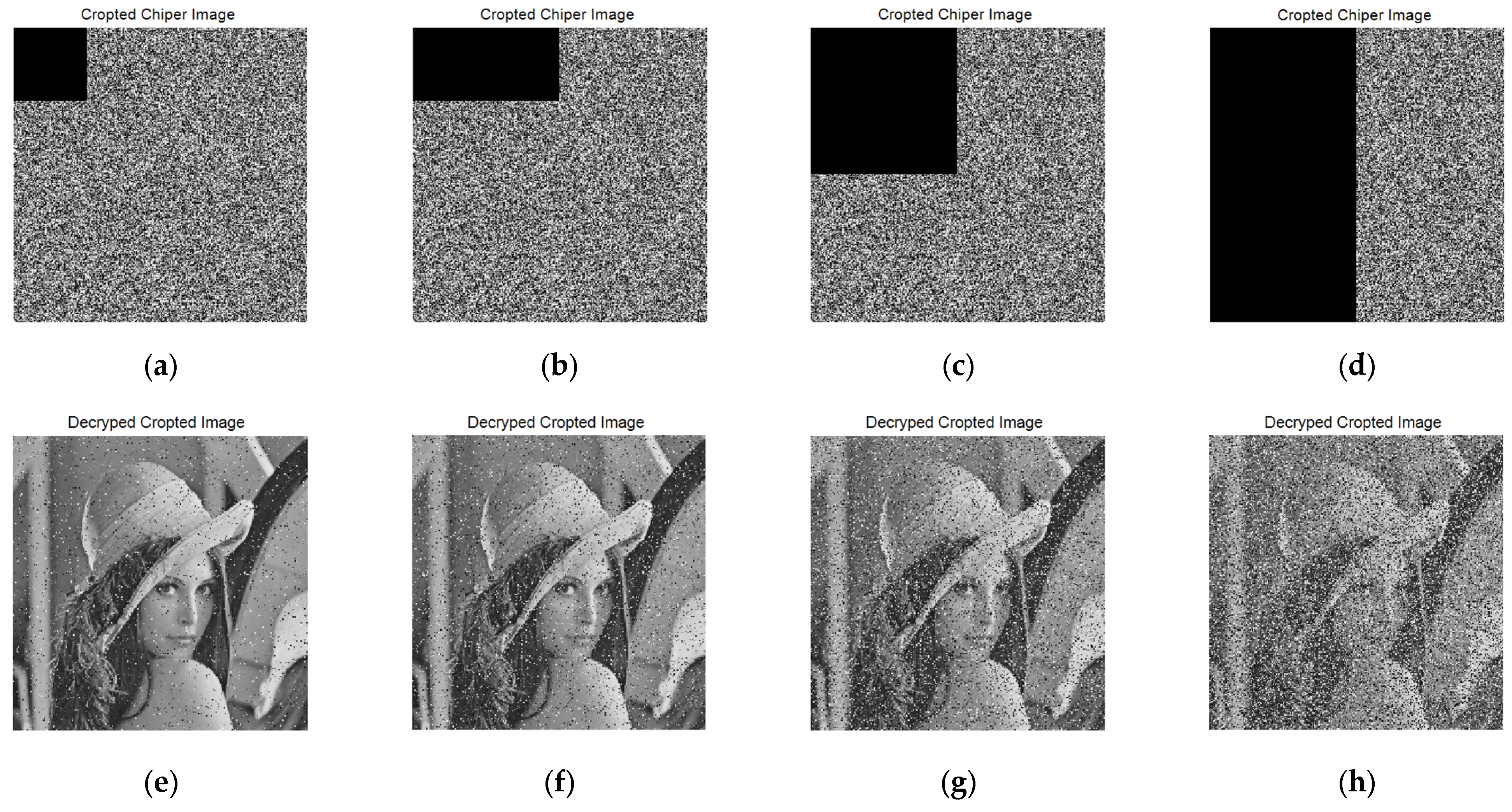
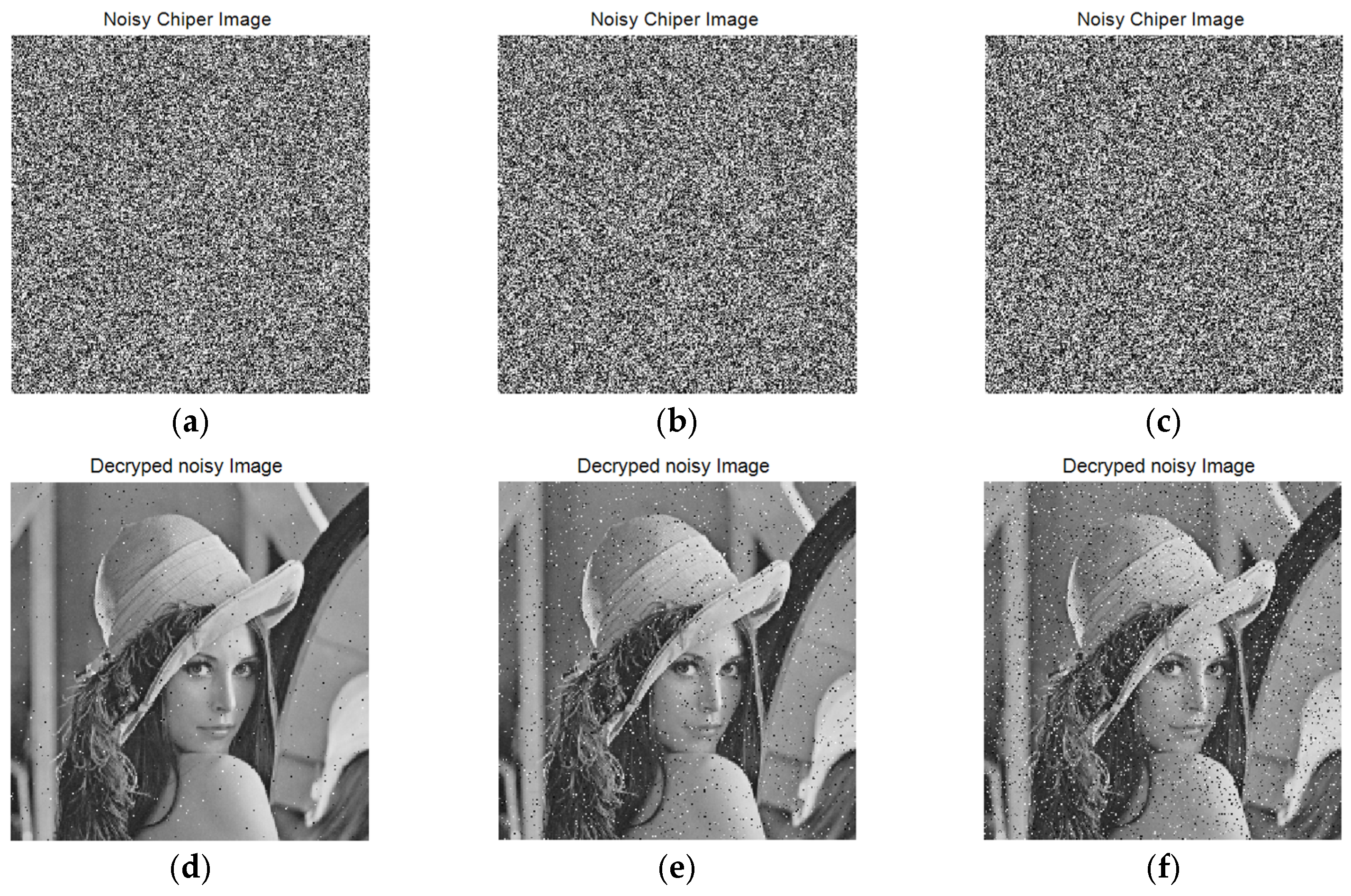
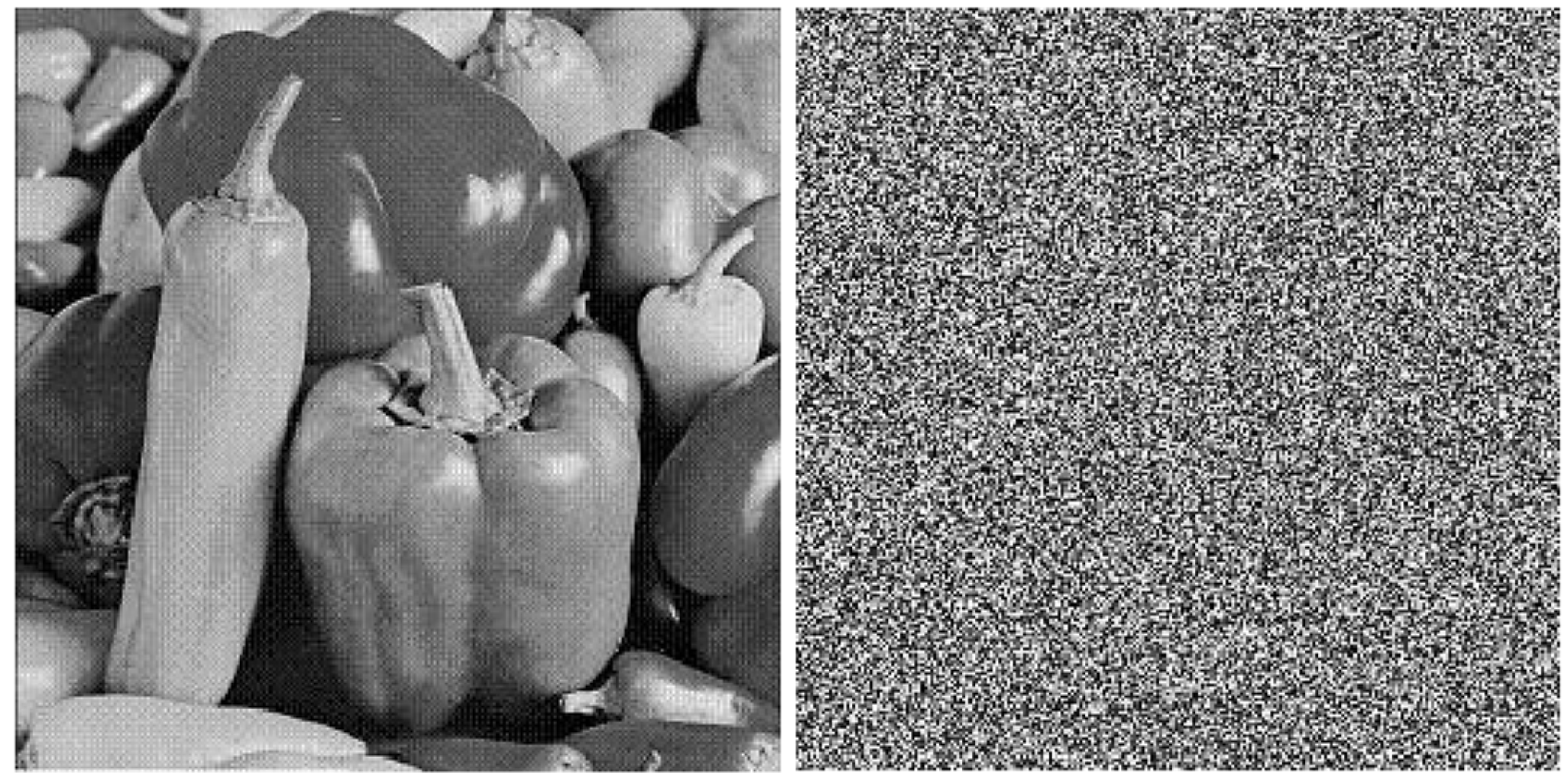
4.7. Anticlipping and Noise Attacks

When the image information is transmitted on the channel, the image information may be subjected to cropping attacks, noise attacks, and other attack methods by the attacker so that the transmitted image information is damaged, and the useful information cannot be obtained after decryption with the correct key. Therefore, we conducted cropping attack and noise attack tests on the images respectively to check the robustness of our algorithm. We used the peak signal-to-noise ratio (PSNR) between the ciphertext image and the plaintext image as a standard [45], and its calculation formula is as Equations (52) and (53):

$$MSE=\frac{{{\displaystyle \sum }}_{i=1}^m{{\displaystyle \sum }}_{j=1}^n{(T_1(i,j)-T_2(i,j))}^2}{m\times n}$$

(52)

$$PSNR=20\ast {log}_{10}(\frac{255}{sqrt(MSE)})$$

(53)

where $m\times n$ is the image size, and $T_1(i,j)$ and $T_2(i,j)$ represent the original image and the encrypted image.

We cropped the image by 1/16, 1/8, 1/4, and 1/2, and set the pixel value of these parts to zero.

Table 6. PSNR of different degrees of clipping attack.

Area	1/16	1/8	1/4	1/2
PSNR	21.314192	18.380856	15.342343	12.250188

shows the peak signal-to-noise ratio (PSNR) of different degrees of cropping attack; Figure 17 shows the decrypted image after the ciphertext is subjected to different degrees of cropping attack. We can see that the general information of the decrypted image can still be identified after being subjected to different degrees of cropping attack; therefore, our algorithm is resistant to clipping attacks.

Then, we applied noise of 0.01, 0.05, and 0.15 intensity to the ciphertext image and decrypted it with the correct key. The PSNR of the decrypted image is shown in

Table 7. PSNR for noise attack.

Noise Level	0.01 Level	0.05 Level	0.1 Level
PSNR	28.971428	22.408105	19.258843

, and the decrypted image is shown in Figure 18, which means that our algorithm is also resistant to noise attacks.

4.8. Key Space Analysis

When the key space is large enough, the algorithm can resist brute force attack. The key in this paper has four parts: initial parameters $d_1~d_8$, $sumP$ of plaintext image pixel values, image block size $Bsize$, supplementary parameters $M1$, $N1$, and the number of blocks Bnum. The calculation accuracy is ${10}^{-15}$. Taking a 256 ∗ 256 image as an example, the main key space is Equation (54):

keyspace = 10¹⁵ ∗ 8 + 10⁸ + 10 + 20 + 10² > 2¹⁰⁰

(54)

Its key space is much larger than $2^{100}$, so it can resist brute force attacks [46].

4.9. Key Sensitivity Analysis

An encryption algorithm is sufficiently secure when it is sensitive to subtle changes in the key, so we tested this on the peppers images. Since our main initial keys $d_1~d_8$ are generated by the SHA-512 function, we randomly selected the correct key $key$, then increased the last digit sequence value generated by SHA-512 by 1, and then calculated and generated a new initial key $key1$, which was only slightly different from the correct key. Figure 19 shows the results of decryption with the changed key, indicating that our method has better key sensitivity.

$key hash value=$ (275afc80927870608dfa79743a56d02e3ff7d009aa78655e9affbcb25e74e1ce102df926ffe0670ca599cc5ef2d57299429bfba3d45b66143fb075b69e590896);

$key=$ (0.385365853658537, 0.412682926829268, 0.578536585365854, 0.237354085603113, 0.038910505836576, 0.578947368421053, 0.578947368421053, 0.290448343079922);

$key1 hash value=$ (275afc80927870608dfa79743a56d02e3ff7d009aa78655e9affbcb25e74e1ce102df926ffe0670ca599cc5ef2d57299429bfba3d45b66143fb075b69e590897);

$key1=$ (0.385365853658537, 0.412682926829268, 0.578536585365854, 0.237354085603113, 0.038910505836576, 0.578947368421053, 0.426900584795322, 0.391812865497076);

4.10. Computational Complexity

Our computational complexity is divided into three parts: generation of initial values, disorder, and diffusion. In the process of generating initial values, we computed them within a constant value $O(m\ast n)$, where $m$ and $n$ denote images and rows and columns, respectively. In the process of dislocation, we dislocated between $Bnum$ layers and $Bisze$ layers, and its computational complexity is a constant value $O(b)$, where $b$ denotes the corresponding maturity. In the process of diffusion, we performed cubic diffusion, whose computational complexity $O(x\ast y\ast z)$, $x,y,z$ are the sizes of the three dimensions of the probability amplitude matrix. With the change of image size and resolution, its computational complexity is $O(m\ast n)+O(x\ast y\ast z)$, which is roughly the same for different images. Therefore, it can be better implemented in practical applications.

5. Conclusions

In this paper, we propose a 3D cuboid image encryption scheme based on message-encoded controlled alternate quantum walks. We used SHA-512 to obtain the key set and used the key set to generate the system parameters of a one-dimensional discrete quantum walk and controlled alternate quantum walk on a circle. Then, we used the one-dimensional discrete quantum walk model and controlled alternating quantum walk model encrypted image to design a three-dimensional cuboid image encryption algorithm. In the scrambling stage, the image was scrambled between layers and layer-by-layer cross-sections; in the diffusion stage, the pixel binary cube was rotated first and combined with the 3D quantum hash, then XORed with the 3D quantum hash sequence and tiled to obtain the encrypted image. Simulation results and image data tests show that the scheme can resist various typical attacks and has good security performance. In the future, we plan to introduce advanced, new technologies and methods [47,48,49,50,51,52], such as deep learning models, neural networks, some concepts of image fusion and recognition, etc. into image encryption and further propose new algorithms with better encryption effects.

References

1. Wan, W.; Wang, J.; Li, J.; Sun, J.; Zhang, H.; Liu, J. Hybrid JND model-guided watermarking method for screen content images. Multimed. Tools Appl. 2020, 79, 4907–4930. [Google Scholar] [CrossRef]
2. Aminuddin, A.; Ernawan, F. AuSR2: Image watermarking technique for authentication and self-recovery with image texture preservation. Comput. Electr. Eng. 2022, 102, 108207. [Google Scholar] [CrossRef]
3. Cao, W.; Mao, Y.; Zhou, Y. Designing a 2D infinite collapse map for image encryption. Signal Process. 2020, 171, 107457. [Google Scholar] [CrossRef]
4. Man, Z.; Li, J.; Di, X.; Sheng, Y.; Liu, Z. Double image encryption algorithm based on neural network and chaos. Chaos Solitons Fractals 2021, 152, 111318. [Google Scholar] [CrossRef]
5. Singh, K.N.; Singh, A.K. Towards integrating image encryption with compression: A survey. ACM Trans. Multimed. Comput. Commun. Appl. 2022, 18, 1–21. [Google Scholar] [CrossRef]
6. Yan, X.; Liu, F.; Yan, W.Q.; Yang, G.; Lu, Y. Weighted visual cryptographic scheme with improved image quality. Multimed. Tools Appl. 2020, 79, 21345–21360. [Google Scholar] [CrossRef]
7. Wang, T.; Wang, M.-H. Hyperchaotic image encryption algorithm based on bit-level permutation and DNA encoding. Opt. Laser Technol. 2020, 132, 106355. [Google Scholar] [CrossRef]
8. Khalil, N.; Sarhan, A.; Alshewimy, M.A. An efficient color/grayscale image encryption scheme based on hybrid chaotic maps. Opt. Laser Technol. 2021, 143, 107326. [Google Scholar] [CrossRef]
9. Zhou, S. A real-time one-time pad DNA-chaos image encryption algorithm based on multiple keys. Opt. Laser Technol. 2021, 143, 107359. [Google Scholar] [CrossRef]
10. Zhang, Y. The fast image encryption algorithm based on lifting scheme and chaos. Inf. Sci. 2020, 520, 177–194. [Google Scholar] [CrossRef]
11. Wang, X.; Guan, N.; Yang, J. Image encryption algorithm with random scrambling based on one-dimensional logistic self-embedding chaotic map. Chaos Solitons Fractals 2021, 150, 111117. [Google Scholar] [CrossRef]
12. Alawida, M.; Teh, J.S.; Samsudin, A. An image encryption scheme based on hybridizing digital chaos and finite state machine. Signal Process. 2019, 164, 249–266. [Google Scholar] [CrossRef]
13. Himeur, Y.; Boukabou, A. A robust and secure key-frames based video watermarking system using chaotic encryption. Multimed. Tools Appl. 2018, 77, 8603–8627. [Google Scholar] [CrossRef]
14. Yu, J.; Xie, W.; Zhong, Z.; Wang, H. Image encryption algorithm based on hyperchaotic system and a new DNA sequence operation. Chaos Solitons Fractals 2022, 162, 112456. [Google Scholar] [CrossRef]
15. Jasra, B.; Moon, A.H. Color image encryption and authentication using dynamic DNA encoding and hyper chatic system. Expert Syst. Appl. 2022, 206, 117861. [Google Scholar] [CrossRef]
16. Qiu, H.; Xu, X.; Jiang, Z.; Sun, K.; Xiao, C. A color image encryption algorithm based on hyperchaotic map and Rubik’s Cube scrambling. Nonlinear Dyn. 2022, 1–19. [Google Scholar] [CrossRef]
17. Mansouri, A.; Wang, X. A novel one-dimensional chaotic map generator and its application in a new index representation-based image encryption scheme. Inf. Sci. 2021, 563, 91–110. [Google Scholar] [CrossRef]
18. Wang, X.; Zhao, M. An image encryption algorithm based on hyperchaotic system and DNA coding. Opt. Laser Technol. 2021, 143, 107316. [Google Scholar] [CrossRef]
19. Xian, Y.; Wang, X. Fractal sorting matrix and its application on chaotic image encryption. Inf. Sci. 2021, 547, 1154–1169. [Google Scholar] [CrossRef]
20. Jithin, K.; Sankar, S. Colour image encryption algorithm combining Arnold map, DNA sequence operation, and a Mandelbrot set. J. Inf. Secur. Appl. 2020, 50, 102428. [Google Scholar] [CrossRef]
21. Gao, W.; Sun, J.; Qiao, W.; Zhang, X. Digital image encryption scheme based on generalized Mandelbrot-Julia set. Optik 2019, 185, 917–929. [Google Scholar] [CrossRef]
22. Gao, Y.; Jiao, S.; Fang, J.; Lei, T.; Xie, Z.; Yuan, X. Multiple-image encryption and hiding with an optical diffractive neural network. Opt. Commun. 2020, 463, 125476. [Google Scholar] [CrossRef] [Green Version]
23. Chen, H.; Liu, Z.; Tanougast, C.; Liu, F. A novel chaos based optical cryptosystem for multiple images using DNA-blend and gyrator transform. Opt. Lasers Eng. 2021, 138, 106448. [Google Scholar] [CrossRef]
24. Wang, F.; Ni, R.; Wang, J.; Zhu, Z.; Hu, Y. Invertible encryption network for optical image cryptosystem. Opt. Lasers Eng. 2022, 149, 106784. [Google Scholar] [CrossRef]
25. Zhang, Y.; Chen, A.; Tang, Y.; Dang, J.; Wang, G. Plaintext-related image encryption algorithm based on perceptron-like network. Inf. Sci. 2020, 526, 180–202. [Google Scholar] [CrossRef]
26. Ding, Y.; Wu, G.; Chen, D.; Zhang, N.; Gong, L.; Cao, M.; Qin, Z. DeepEDN: A deep-learning-based image encryption and decryption network for internet of medical things. IEEE Internet Things J. 2020, 8, 1504–1518. [Google Scholar] [CrossRef]
27. Yu, F.; Zhang, Z.; Shen, H.; Huang, Y.; Cai, S.; Du, S. FPGA implementation and image encryption application of a new PRNG based on a memristive Hopfield neural network with a special activation gradient. Chin. Phys. B 2022, 31, 020505. [Google Scholar] [CrossRef]
28. Shi, Y.; Hu, Y.; Wang, B. Image encryption scheme based on multiscale block compressed sensing and Markov model. Entropy 2021, 23, 1297. [Google Scholar] [CrossRef]
29. Sun, C.; Wang, E.; Zhao, B. Image encryption scheme with compressed sensing based on a new six-dimensional non-degenerate discrete hyperchaotic system and plaintext-related scrambling. Entropy 2021, 23, 291. [Google Scholar] [CrossRef]
30. Wang, X.; Li, Y. Chaotic image encryption algorithm based on hybrid multi-objective particle swarm optimization and DNA sequence. Opt. Lasers Eng. 2021, 137, 106393. [Google Scholar] [CrossRef]
31. Abbasi, A.A.; Mazinani, M.; Hosseini, R. Chaotic evolutionary-based image encryption using RNA codons and amino acid truth table. Opt. Laser Technol. 2020, 132, 106465. [Google Scholar] [CrossRef]
32. Liang, Z.; Qin, Q.; Zhou, C. An image encryption algorithm based on Fibonacci Q-matrix and genetic algorithm. Neural Comput. Appl. 2022, 34, 19313–19341. [Google Scholar] [CrossRef]
33. Liu, X.; Xiao, D.; Huang, W.; Liu, C. Quantum block image encryption based on arnold transform and sine chaotification model. IEEE Access 2019, 7, 57188–57199. [Google Scholar] [CrossRef]
34. Wang, J.; Chen, J.; Wang, F.; Ni, R. Optical image encryption scheme based on quantum s-box and meaningful ciphertext generation algorithm. Opt. Commun. 2022, 525, 128834. [Google Scholar] [CrossRef]
35. Ma, Y.; Li, N.; Zhang, W.; Wang, S.; Ma, H. Image encryption scheme based on alternate quantum walks and discrete cosine transform. Opt. Express 2021, 29, 28338–28351. [Google Scholar] [CrossRef] [PubMed]
36. Khan, M.; Hussain, I.; Jamal, S.S.; Amin, M. A privacy scheme for digital images based on quantum particles. Int. J. Theor. Phys. 2019, 58, 4293–4310. [Google Scholar] [CrossRef]
37. Yan, T.; Li, D. A Novel Quantum Color Image Encryption Scheme Based on Controlled Alternate Quantum Walks. In Proceedings of the International Conference on Security, Privacy and Anonymity in Computation, Communication and Storage, New York, NY, USA, 9–13 August 2021; Springer: Cham, Switzerland, 2021; pp. 519–530. [Google Scholar]
38. Yang, Y.-G.; Pan, Q.-X.; Sun, S.-J.; Xu, P. Novel image encryption based on quantum walks. Sci. Rep. 2015, 5, 7784. [Google Scholar] [CrossRef] [PubMed] [Green Version]
39. Yang, Y.-G.; Xu, P.; Yang, R.; Zhou, Y.-H.; Shi, W.-M. Quantum Hash function and its application to privacy amplification in quantum key distribution, pseudo-random number generation and image encryption. Sci. Rep. 2016, 6, 19788. [Google Scholar] [CrossRef] [PubMed] [Green Version]
40. Abd EL-Latif, A.A.; Abd-El-Atty, B.; Abou-Nassar, E.M.; Venegas-Andraca, S.E. Controlled alternate quantum walks based privacy preserving healthcare images in internet of things. Opt. Laser Technol. 2020, 124, 105942. [Google Scholar] [CrossRef]
41. Abd EL-Latif, A.A.; Abd-El-Atty, B.; Venegas-Andraca, S.E. Controlled alternate quantum walk-based pseudo-random number generator and its application to quantum color image encryption. Phys. A Stat. Mech. Appl. 2020, 547, 123869. [Google Scholar] [CrossRef]
42. Boriga, R.E.; Dăscălescu, A.C.; Diaconu, A.V. A new fast image encryption scheme based on 2D chaotic maps. IAENG Int. J. Comput. Sci. 2014, 41, 249–258. [Google Scholar]
43. Shannon, C.E. A mathematical theory of communication. Bell Syst. Tech. J. 1948, 27, 379–423. [Google Scholar] [CrossRef] [Green Version]
44. Wu, Y.; Noonan, J.P.; Agaian, S. NPCR and UACI randomness tests for image encryption. Cyber J. Multidiscip. J. Sci. Technol. J. Sel. Areas Telecommun. 2011, 1, 31–38. [Google Scholar]
45. Hore, A.; Ziou, D. Image Quality Metrics: PSNR vs. SSIM. In Proceedings of the 2010 20th International Conference on Pattern Recognition, Istanbul, Turkey, 23–26 August 2010; pp. 2366–2369. [Google Scholar]
46. Alvarez, G.; Li, S. Some basic cryptographic requirements for chaos-based cryptosystems. Int. J. Bifurc. Chaos 2006, 16, 2129–2151. [Google Scholar] [CrossRef] [Green Version]
47. Li, Y. Research and Application of Deep Learning in Image Recognition. In Proceedings of the 2022 IEEE 2nd International Conference on Power, Electronics and Computer Applications (ICPECA), Shenyang, China, 21–23 January 2022; pp. 994–999. [Google Scholar]
48. Falcetta, A.; Roveri, M. Privacy-preserving deep learning with homomorphic encryption: An introduction. IEEE Comput. Intell. Mag. 2022, 17, 14–25. [Google Scholar] [CrossRef]
49. Chen, J.; Qiu, X.; Ding, C.; Wu, Y. SAR image classification based on spiking neural network through spike-time dependent plasticity and gradient descent. ISPRS J. Photogramm. Remote Sens. 2022, 188, 109–124. [Google Scholar] [CrossRef]
50. Yan, S.; Gu, Z.; Park, J.H.; Xie, X. Synchronization of delayed fuzzy neural networks with probabilistic communication delay and its application to image encryption. IEEE Trans. Fuzzy Syst. 2022. [Google Scholar] [CrossRef]
51. Li, J.; Liu, J.; Zhou, S.; Zhang, Q.; Kasabov, N.K. Learning a coordinated network for detail-refinement multi-exposure image fusion. IEEE Trans. Circuits Syst. Video Technol. 2022. [Google Scholar] [CrossRef]
52. Feng, L.; Chen, X. Image recognition and encryption algorithm based on artificial neural network and multidimensional chaotic sequence. Comput. Intell. Neurosci. 2022, 2022, 9576184. [Google Scholar] [CrossRef]
Figure 1. 1D discrete quantum walk probability distribution on a circle.
Mathematics 10 04441 g001
Figure 2. Controlled alternate quantum walk probability distribution on a circle.
Mathematics 10 04441 g002
Figure 3. A 3D Cuboid Image Encryption Framework Based on Message-Encoded Controlled Alternate Quantum Walks.
Mathematics 10 04441 g003
Figure 4. Generation of image cuboid.
Mathematics 10 04441 g004
Figure 5. Generation of index sequence p r m 1 D t .
Mathematics 10 04441 g005
Figure 6. Interlayer scrambling of image cuboids.
Mathematics 10 04441 g006
Figure 7. Top-down layer-by-layer scrambling based on 3D probability distribution matrix.
Mathematics 10 04441 g007
Figure 8. Binary cube rotation based on probability magnitude matrix.
Mathematics 10 04441 g008
Figure 9. Simulation results (256 ∗ 256): (ae) original images; (fj) encrypted images; (ko) decrypted images.
Mathematics 10 04441 g009
Figure 10. Simulation results (512 ∗ 512 and irregular): (ad) original images; (eh) encrypted images; (il) decrypted images.
Mathematics 10 04441 g010aMathematics 10 04441 g010b
Figure 11. Histogram Analysis (256 ∗ 256): (ac) original images; (df) encrypted image.
Mathematics 10 04441 g011
Figure 12. Histogram Analysis (512 ∗ 512 and irregular): (ad) original images; (eh) encrypted image.
Mathematics 10 04441 g012
Figure 13. Correlation of different ciphertext images.
Mathematics 10 04441 g013
Figure 14. Adjacent pixel correlation of image 5.1.09: (ac) original image; (df) encrypted image.
Mathematics 10 04441 g014aMathematics 10 04441 g014b
Figure 15. Adjacent pixel correlation of image 5.2.08: (ac) original image; (df) encrypted image.
Mathematics 10 04441 g015
Figure 16. Adjacent pixel correlation of image 5.3.01: (ac) original image; (df) encrypted image.
Mathematics 10 04441 g016aMathematics 10 04441 g016b
Figure 17. Decrypted images for varying degrees of cropping attacks: (a) 1/16 crop; (b) 1/8 crop; (c) 1/4 crop; (d) 1/2 crop; (eh) decrypted images of (ad).
Mathematics 10 04441 g017
Figure 18. Noise attack test results: (ac) noisy cipher image of different noise level; (df) decrypted noisy image.
Mathematics 10 04441 g018
Figure 19. Decryption result of correct key k e y and changed key k e y 1 .
Mathematics 10 04441 g019