Abstract
The total heat exchange factor is one of the most important thermal physical parameters in the heat transfer model for a reheating furnace machine. In this paper, a novel general strategy, which is combined with the first-optimize-then-discretize (FOTD) approach and an improved hybrid conjugate gradient (IHCG) algorithm, is proposed to identify the total heat exchange factor by solving a nonlinear inverse heat conduction problem (IHCP). Firstly, a nonlinear IHCP with the Dirichlet-type boundary condition is built to determine the unknown total heat exchange factor . Secondly, the analysis of the Fréchet gradient of the cost functional is given and the gradient is proved as Lipschitz continuous by the FOTD approach. Thirdly, based on the gradient information by FOTD, a new IHCG algorithm, whose global convergence is proved by us, is proposed for fast solving of the optimization problem. Finally, simulation experiments are given to verify the effectiveness of the proposed strategy. Compared with the first-discretize-then-optimize (FDTO) approach, the FOTD approach can reduce running time and iteration number. Compared with other CG algorithms, the proposed IHCG algorithm has better convergence performance. The experimental data by the thermocouples experiments from a reheating furnace are also given to identify the total heat exchange factor.
Keywords:
first-optimize-then-discretize; hybrid conjugate gradient algorithm; inverse heat conduction problem; lipschitz continuity; nonlinear PDEs; total heat exchange factor MSC:
35K05
1. Introduction
The method of total heat exchange factor is often used to build the temperature prediction model for the reheating furnace, and has been widely used in the online control due to its simplicity and lower computer cost [1]. The total heat exchange factor is one of the most important thermal physical parameters. It has significant effects on the accuracy of temperature fields in the calculation process of the prediction model [2]. However, the determination of the total heat exchange factor is very complicated due to the complex environment, in which many various factors (such as: structural parameters, operating parameters, thermal parameters, etc.) should be considered. Generally, the inverse heat conduction problem (IHCP), in which some characteristics are unknown, is often used to determine the unknown parameters. For instance, the unknown temperature-dependent parameters (such as: local convective heat transfer coefficients [3], surface heat flux [4,5], thermal conductivity [6], surface heat sources [7], etc.) can be evaluated in the solution of IHCP. Thus, a new IHCP is built to determine the total heat exchange factor, and it should be solved both quickly and accurately in this paper.
Methods for solving the IHCP include the conjugate gradient (CG) method [6], the maximum entropy (ME) method [8], the neural network (NN) method [9] and so on. These algorithms can be generally classified into two categories: the stochastic intelligent algorithms and the gradient-based algorithms [10]. The disadvantage of the stochastic intelligent methods is the low computation efficiency. Especially, a large number of iterations are required and only few parameters can be reconstructed [11]. The advantages of the gradient-based methods are the fast convergence speed and the high accuracy. However, it is not easy to obtain the gradient information for real applications. Since we want to solve the IHCP quickly and accurately, the gradient-based method is chosen to construct an effective gradient-based algorithm in this paper.
Current gradient-based numerical methods are divided into two groups: the first-discretize-then-optimize (FDTO) approach with the sensitivity matrix and the first-optimize-then-discretize (FOTD) approach with the adjoint equation [12]. In the past few decades, researchers pay more attention to the FDTO approach with the sensitivity matrix, and proposed a variety of numerical algorithms. For instance, Tseng et al. [13] developed a direct sensitivity coefficient (DSC) method to solve multidimensional IHCPs. Anderson et al. [14] determined the effective heat transfer coefficients by using an inverse method, in which the sensitivity coefficient is solved in an iterative manner. Han et al. [15] used the finite element method (FEM) to solve the sensitivity matrix, and the sensitivity analysis of the transient IHCP is carried out in this paper. Cui et al. [16] presented a complex variable differentiation method (CVDM) for accurately calculating sensitivity coefficients for a Levenberg–Marquardt (LM) algorithm to solve IHCPs. Zhang et al. [17] calculated the sensitivity matrix coefficients by the newly developing FEM and CVDM though ABAQUS. In general, sensitivity coefficients are difficult to accurately calculate. Besides, if the IHCP has some other properties (such as: multi-dimensions, transient states or nonlinearities), the calculation process will be a more difficult and challenging work.
Recently, some researchers have proposed a series of FOTD approaches and successfully introduced them into IHCPs. For instance, Azar et al. [18] proposed an iterative regularization method, in which the adjoint equation is given to determine the gradient of the cost function, to identify the unknown parameter by solving the IHCP. Xiong et al. [5] proposed a sequential CG method to reconstruct the undetermined surface heat flux for nonlinear IHCP. The adjoint partial differential equation (PDE) is introduced to describe the gradient of the objective function. On the bases of our earlier studies [19,20], an improved hybrid conjugate gradient (IHCG) algorithm based on the FOTD approach is proposed to determine the unknown total heat exchange factor by solving the IHCP with the Dirichlet-type boundary condition .
This paper is composed as follows. In Section 2, mathematical models of reheating furnace and a nonlinear inverse heat conduction problem are built. Based on the FOTD approach, the explicit formula for the Fréchet gradient of the cost function is obtained, and the Lipschitz continuity of the gradient is proved in Section 3. In Section 4, an improved hybrid conjugate gradient (IHCG) algorithm is given, and a detailed mathematics proof of global convergence is published. In Section 5, simulation experiment and analysis are given to verify the effectiveness of the FOTD approach and the proposed IHCG algorithm. The experimental data by the thermocouples experiments are also given to identify the total heat exchange factor for the furnace. Finally, the conclusion is summarized in Section 6.
2. Problem Formulation
2.1. Mathematical Model for the Reheating Furnace
The heat transferred to the slab is extremely complicated. It is mainly in the form of heat convection, heat conduction and thermal radiation, as shown in Figure 1. To solve the model in practical engineering applications, some assumptions are given to build a low-dimensional mathematical model: 1. The heat conduction inside the slab is only transferred along the slab’s thickness direction. Because the temperature difference along the length and width direction is much smaller than the slab’s thickness direction [19]. 2. Thermal radiation is the only considered mode of heat exchange between the slabs and their environment. Other heat transfers such as conduction, skid marks, oxide scale layer, etc., are omitted [21]. 3. A half part of the slab is considered for the mathematical model. As the slab is symmetrically heated approximately in the furnace [4]. Finally, the 1-dimensional transient nonlinear mathematical model with the temperature-dependent material parameters is considered and shown as Equation (1). In this analysis, neither source term nor phase change inside the solid are considered.
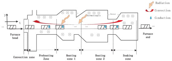
Figure 1.
The structure of the reheating furnace.
Here, is the temperature field in the slab along the thickness dimension y with . The symbol l is the thickness of the slab , and and are the charging and discharging time of the slab. is the slab’s charging temperature (K), and is the Stefan–Boltzmann constant, (W/m K). The symbol defines the heat flux density, which is determined by the total heat exchange factor , upper furnace temperatures , and slab’s upper surface temperature . Furthermore, is density (kg/m), and are the specific heat (J/(kg·K)) and the thermal conductivity (W/(m·K)), respectively. According to the paper [22], and are temperature-dependent and shown in Figure 2 for the 20MnSi steel slab.
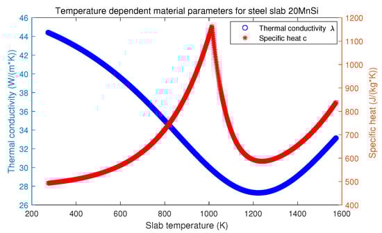
Figure 2.
Temperature dependent material parameters for steel slab 20MnSi.
As verified in [23,24], a time-invariant transformation function, , is chosen to isolate the nonlinear material characteristics in Equation (1). Then, after utilization of the transformation law into PDEs (1), the new PDE equations are obtained:
Here, , , ; still defines the heat flux density, which does not depend on y.
2.2. Inverse Heat Conduction Problem
To obtain more accurate measurement data, the slab is equipped with a set of thermocouples to go through the reheating process [20]. The center temperatures in the slab are seldom affected by the environment relative to the surface temperatures. Thus, the measured output data can be used as the Dirichlet-type boundary condition in this paper. Then, the IHCP can be described by the following PDEs-constrained optimization problem:
3. The Fréchet Gradient Based on the FOTD Approach
In this section, the FOTD approach based on the adjoint equation is introduced to obtain the Fréchet gradient of the cost functional. Afterward, the Lipschitz continuous is proved.
3.1. The Adjoint PDEs Based on Weak Solutions
To derive the adjoint PDEs, the Lagrange function-based approach [12] is applied. is introduced to transfer all constraints into cost functional and formulate the strong version of the Lagrange function, which is shown as:
From the book [12], the adjoint equation is obtained by solving for . It is shown as:
Denote by are the solutions of problem (2). Then, will be the weak solution of the following parabolic problem:
3.2. Fréchet Gradient of the Cost Functional
The first variation of the cost functional (3) is obtained as:
By the FOTD approach, an explicit formula for the gradient of the cost functional will be defined by the solution of the adjoint Equation (5). A simple derivation for the first term of the right-hand of Equation (7) is given in Lemma 1.
Lemma 1.
Proof.
From the boundary conditions of Equation (5), the left-hand side of Equation (8) can be rewritten as:
Lemma 1 is proved. □
Then, Lemma 2 is given and proved for the second term of the right-hand of Equation (7).
Lemma 2.
Let be the solution of the parabolic problem (6) for a given . Then, the following equation with a constant is obtained:
where , , , , , and .
Proof.
Multiply both sides of by , and integrate over , we can obtain the following equation:
By , the left-hand of Equation (12) can be transferred as:
The right-hand of Equation (12) can be converted to the following equation:
Then, the -inequality: is introduced for the right-hand side of Equation (15), which is converted to the following inequality:
Equation (17) requires . Then, with , we can obtain two inequalities:
Finally, with , we obtain the following estimate:
Theorem 1.
Let Lemmas 1 and 2 hold. Then the cost functional is the Fréchet -differential . Moreover, the Fréchet derivative of the cost functional at can be defined by the solution of the adjoint Equation (5) as follows:
3.3. Lipschitz Continuous
Using lemmas in the previous section, we can show that the gradient of the cost functional is Lipschitz continuous.
Lemma 3.
Let the condition of Theorem 1 hold. Then, there is a constant to make the following inequality hold:
where, , , , , , and,
The process of proof is shown in Appendix A.
4. The Improved Hybrid Conjugate Gradient Algorithm
In Section 3, the gradient can be calculated by the formula (20) based on the FOTD approach. This suggests an idea of constructing a new gradient-based optimization algorithm based on the FOTD approach.
There are many innovative CG algorithms with different values of , such as the LS algorithm [25], HS algorithm [26], MCD algorithm [27], the variant Flétcher–Reeves (VFR) algorithm [28], the modified Polak–Ribière–Polyak (MPRP) algorithm [29], the spectral conjugate gradient (SCG) algorithm [30], the Nonlinear three-term conjugate gradient (NTTCG) algorithm [31]. In the past few years, some hybrid algorithms [32,33,34,35] have been developed based on the above algorithms. Inspired by these CG algorithms, this paper presents an improved hybrid conjugate gradient (IHCG) algorithm, which is given as follows:
where,
Here, represents the gradient by Equation (20). The flowchart of IHCG algorithm is shown in Algorithm 1.
| Algorithm 1: IHCG algorithm based on the FOTD approach. | |
| Begin | |
| 1: | Set parameters . Choose an initial point . |
| 2: | Solve the direct problem (2) to determine the temperature distribution , and estimate the cost function ; |
| 3: | Solve the adjoint problem (5) to determine the gradient of the cost function . If or , stop the algorithm. |
| 4: | Estimate the descent depth based on and Equation (23). |
| 5: | Determine a step length by the standard Wolfe line search method.
|
| 6: | Update , and go to Step 2. |
| end | |
4.1. Property of the Proposed Algorithm
In this section, the global convergence of Algorithm 1 is proved under the Wolfe line search condition (25). Sufficient descent property is very important for the global convergence of the iterative method [36]. The following lemmas are given to state that the search directions in Algorithm 1 are all of descent.
Lemma 4.
Proof.
Obviously, when . When , we divide the proof into the two situations by .
Situation 1: If and , we can obtain .
Situation 2: If and , the proof is divided by the following four cases:
Case 1: If and , we can obtain that . Then, the following inequality is derived:
Case 2: If and , we can obtain that . The following inequality is derived:
Case 3: If and , we can obtain that . Notice, that we have , where is the angle between and . The following inequality is derived:
Case 4: If and , we can obtain and . The following inequality is derived:
Finally, for all , always holds. □
Meanwhile, we can easily obtain the following important property.
Lemma 5.
For any , the relation always holds.
Proof.
From the definition of in Equation (23), one knows . Next, we divide the proof into the two situations by .
Situation 1: If , by Lemma 4, we can obtain .
Situation 2: If , the proof is divided by the following four cases:
Case 1: If and , from Lemma 4.1 and Equation (27), we have:
Case 2: If and , from Lemma 4.1 and Equation (28), we have: , then the following inequality is obtained.
Case 3: If and , from Lemma 4.1 and Equation (29), we have:
Case 4: If and , from Lemma 4.1 and Equation (30), we have , and the following inequality is obtained.
Finally, Lemma 5 is proved. □
4.2. Global Convergence
As demonstrated in [34], the following assumptions are needed to prove the global convergence:
1. The objective function is bounded from below on the level set , where , and is the initial point.
2. The gradient of the cost functional is Lipchitz continuous and a constant exists, which has been given by Lemma 3.
Lemma 6.
Suppose that Assumptions 1 and 2 hold. Considering the iteration , the direction and step length satisfy the Wolfe line search condition (25), we can obtain:
Proof.
By contradiction, if Equation (36) does not hold, there exists a positive constant satisfying for all . From and Lemma 5, we can obtain:
Divided both sides of Equation (37) by , the following equation is obtained:
By a recurrence of Equation (38) and , we can have:
It concludes that , which contradicts with Equation (35), so Lemma 6 is proved. □
5. Simulation and Analysis
In this section, some simulations are made to verify the proposed IHCG algorithm based on the FOTD approach. Firstly, the comparison between the FDTO approach and FOTD approach is given. Secondly, the comparison between IHCG and other popular variant CG algorithms (LS [25], HS [26], MCD [27], VFR [28], MPRP [29], SCG [30], NTTCG [31]) is given. Finally, the application of the reheating furnace with actual measured data is considered to identify the total heat exchange factor. All simulations are programmed by MATLAB R2018b and implemented on a computer with Intel i5-11400F GPU, 2.60 GHz, 16GB RAM.
5.1. FOTD Approach vs. FDTO Approach
Here, the FDTO approach is introduced as the comparative object. In the FDTO approach, the explicit finite difference method [37] is used to discretize the direct PDEs (2). By the FDTO approach with the sensitivity method [12], the gradient is obtained in terms of the Jacobian matrix: , where, is the discrete form of : , and n is the total number of discrete points. Generally, times solution of nonlinear PDEs (2) are required to calculate the Jacobian matrix.
In this case, the total heat exchange factor of PDEs (2) is defined as the functional form: . Furthermore, other parameter values of the PDE Equation (2) are shown as: (m), (K), (kg/m), (min). Then, the accurate measured values of the center temperature are obtained by solving the direct PDEs (2) with . The initial value of is given as . The details of in forms of the sine function are illustrated in Figure 3. The same numerical algorithm (LS [25]) is applied for both the FDTO and FOTD approaches. The numerical values of the computational results are given in Figure 4 and Table 1.
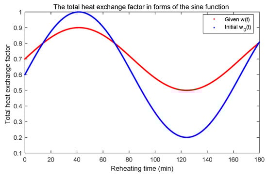
Figure 3.
The total heat exchange factor in forms of the sine function.
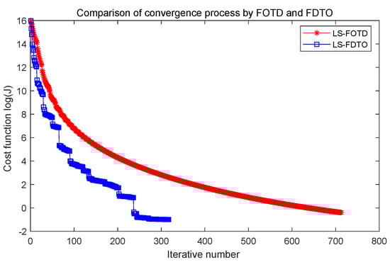
Figure 4.
Comparison of convergence process by FOTD and FDTO approaches.

Table 1.
Comparison of simulation performance between FOTD and FDTO approaches.
Combing Figure 4 and Table 1, it is clear that the FDTO approach yields less iteration steps than the FOTD approach; meanwhile, the value of the final cost functional J is a little smaller than the FOTD approach. However, the simulation time of the FDTO approach is 42035.76 s, which is 140 times larger than the 300.92 s by the FOTD approach because it wastes exceedingly large computation time to obtain times the solution of nonlinear PDEs for the Jacobian matrix of the FDTO approach.
In general, the FOTD approach takes less time to obtain the almost same value of the final cost functional than the FDTO approach.
5.2. Comparisons between IHCG and Other CG Algorithms
The proposed IHCG algorithm is compared with other popular variant CG algorithms (LS [25], HS [26], MCD [27], VFR [28], MPRP [29], SCG [30], NTTCG [31]). Here, the comparisons are shown in the following two cases.
Case 1: In this case, the physical parameters of Section 5.1 are used. The numerical performances of the computational results are given in Figure 5, Figure 6 and Figure 7 and Table 2. Notice, the Y-coordinate direction is a logarithmic function of the cost function in Figure 6.
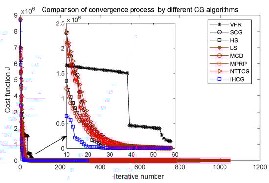
Figure 5.
Comparison of convergence process J by different CG algorithms.
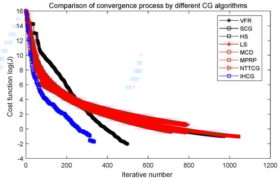
Figure 6.
Comparison of convergence process by different CG algorithms.
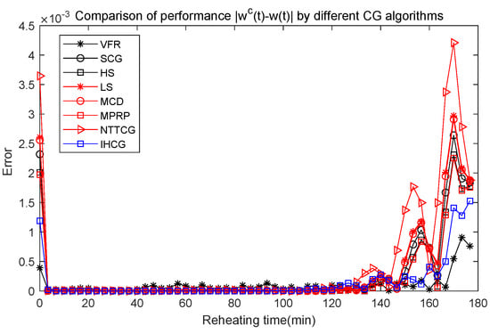
Figure 7.
Comparison of performance by different CG algorithms.
Table 2.
Comparison of simulation performance by different CG algorithms.
Figure 5 shows that the performance of our proposed IHCG is better than other CG algorithms in the early stage of the converged process, and Figure 6 shows that our proposed IHCG needs less iteration steps (only 334) to satisfy the convergence criteria, which is much lower than all the other CG algorithms. Combining Table 2, the running time by our proposed IHCG is 140.38 s, which is lower than all the other CG algorithms.
The symbol in Figure 7 means the absolute prediction errors by different CG algorithms. In Figure 7, the smallest two prediction errors are obtained by by the VFR algorithm and our IHCG algorithm. However, the iteration steps and simulation time by the VFR algorithm are much bigger than that by the IHCG algorithm as shown in Table 2. Notice, there is a phenomenon in Figure 7 that the prediction errors near the final time are relatively higher than other periods. This phenomenon may be caused by the FOTD approach, in which the Fréchet gradient at the final time is strongly effected by from the weak solution of the adjoint PDE (2).
Compared with other CG algorithms, the proposed IHCG algorithm can solve the IHCP quickly and accurately.
Case 2: In this case, the physical parameters of Section 5.1 are also used. Furthermore, some errors are added for the measured values . It assumes that the temperature values at 10 points are known with random errors:
Considering the measured values with errors, the IHCG and other CG algorithms are used to identify the given , and the simulation results are given in Table 3 and Figure 8, Figure 9 and Figure 10. In Table 3, S denotes the standard deviation, and is the maximum standard deviation [35]. They are defined as:
where is the calculated value by solving the IHCP (3), is the true measured value with random errors, and is the total number of cells for the whole reheating time.
Table 3.
Comparison under different error levels by different CG algorithms.
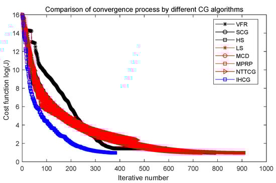
Figure 8.
Comparison of convergence process by different CG algorithms ().
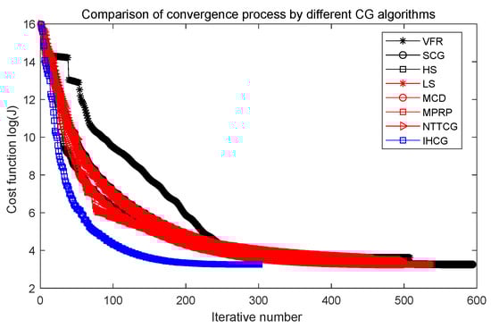
Figure 9.
Comparison of convergence process by different CG algorithms ().
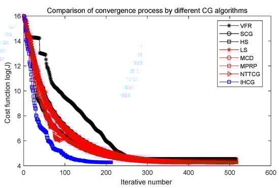
Figure 10.
Comparison of convergence process by different CG algorithms ().
In Table 3, the best values are shown in bold. The smallest values of S and are obtained by the VFR algorithm when the random errors are given by . Except for the VFR algorithm, the IHCG algorithm performs better than all the other CG algorithms. With the increase of the random errors , the smallest values of S and are obtained by the IHCG algorithm, which means the proposed IHCG algorithm can overcome the bad affect caused by random errors for the inverse heat conduction problem.
In contrast to other CG algorithms, the IHCG algorithm needs the smallest iteration step to accelerate the convergence rate as shown in Figure 8, Figure 9 and Figure 10. This goes to prove that the IHCG algorithm can solve the proposed IHCP quickly.
Finally, the IHCG algorithm can effectively eliminate the ill-posedness of the inverse problem.
5.3. Application in Reheating Furnace
In this case, the measured values of the center temperature were obtained from a walking beam reheating furnace. The charging state and discharging state of the trial steel slab, whose thickness is m, is shown in Figure 11. The slab enters into the reheating furnace at 15:40, and is discharged from the furnace at 18:13. Thus, the total reheating time is 153 min. In the trial steel slab, the thermocouples (Type K, mm) are set to record the center and surface temperatures of the slab. The center temperatures are shown in Figure 12 and defined as Dirichlet type boundary condition to obtain and identify the total heat exchange factor. The identified total heat exchange factor will be introduced into the transient nonlinear heat conduction model in Section 2. The measured surface temperatures in Figure 12 will be compared with the calculated surface temperatures to verify the necessity and accuracy of identifying the total heat exchange factor.
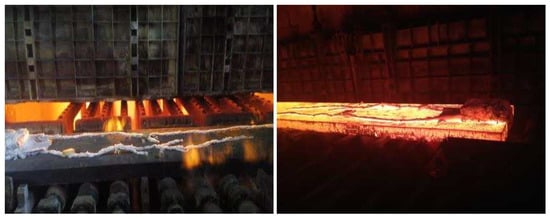
Figure 11.
Charging and discharging state of the trial steel slab.
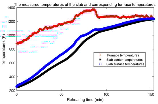
Figure 12.
The measured center and surface temperature of the slab and corresponding furnace temperatures.
First, the IHCG and other CG algorithms are used to identify the total heat exchange factor based on actual measured data. The initial guess is also defined as the functional form: . The convergence rate of these algorithms is shown in Figure 13, and the iterative number and running time are listed in Table 4. In Figure 13 and Table 4, the VFR and NTTCG algorithm cannot obtain enough small cost function J when the convergence process is stopped at . The IHCG algorithm performs best among these CG algorithms. It needs 407.42 s to obtain the value of cost function J is 7.58 when the convergence process is stopped at 781 iteration steps. The identified total heat exchange factor by IHCG algorithm based on actual measured data is shown in Figure 14.
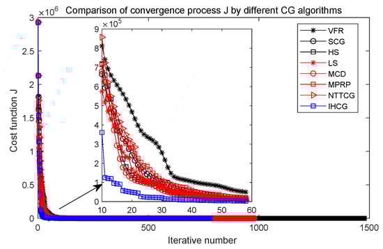
Figure 13.
Comparison of convergence process J by different CG algorithms by actual measured data.
Table 4.
Comparison of simulation performance by different CG algorithms with measured data.
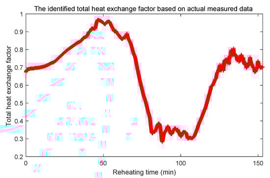
Figure 14.
The identified total heat exchange factor based on actual measured data.
Second, the PDE model with the identified total heat exchange factor in Figure 14 is solved to calculate the surface temperature. Here, a new PDE model, in which the total heat exchange factor is given as constant , is introduced as the comparative object. The calculated surface temperatures by two PDE models are compared with the measured surface temperatures, which is shown in Figure 15. In Figure 15, is the measured surface temperatures, stands for the calculated surface temperatures with the identified total heat exchange factor, and represents the calculated surface temperatures with the constant . The temperature differences with different total heat exchange factors are shown in Figure 16. It is clear the calculated surface temperatures with the identified total heat exchange factor are closer to the measured surface temperatures than that with the constant .
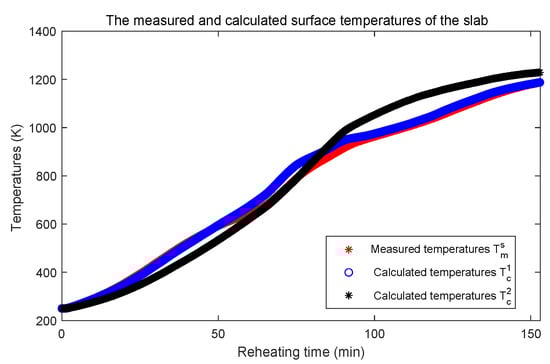
Figure 15.
The calculated surface temperatures by two PDE models.
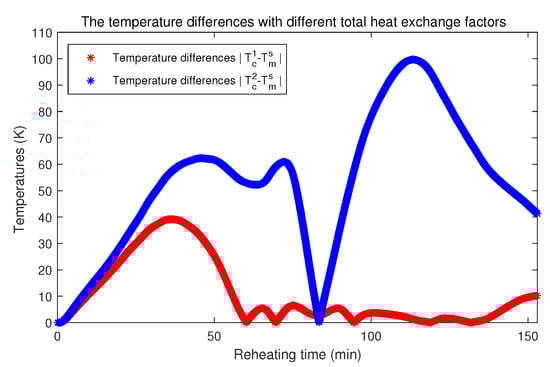
Figure 16.
The temperature differences with different total heat exchange factors.
6. Conclusions
In the present work, a new strategy combined the FOTD approach and a new IHCG algorithm is proposed to identify the total heat exchange factor for the reheating furnace by solving a typical inverse heat conduction problem. The main contributions of this paper are given as follows:
1. A nonlinear IHCP with the Dirichlet-type boundary condition is proposed to identify the unknown total heat exchange factor for the reheating furnace.
2. The FOTD approach is applied to obtain the Fréchet gradient of the cost function, which can be described by the weak solution of the adjoint equations. Simulation results prove that the FOTD approach takes less time to obtain nearly the same value of the final cost functional than the FDTO approach.
3. Based on the Fréchet gradient of the cost function by the FOTD approach, a new IHCG algorithm, which combines the hybrid scalar parameter with spectrum , is developed for the numerical solution of the proposed IHCP. The simulation results show that the IHCG algorithm is accurate and can effectively eliminate the ill-posedness of the inverse problem.
Moreover, the new strategy may provide a theoretical basis for identifying the unknown thermophysical properties for other applications.
Author Contributions
Conceptualization, M.L., X.L. and Z.Y.; methodology, Z.Y.; software, M.L. and P.L.; validation, M.L. and J.Q.; formal analysis, Z.Y.; investigation, Z.Y.; resources, X.L.; data curation, M.L.; writing—original draft preparation, Z.Y.; writing—review and editing, Z.Y.; visualization, Z.Y.; supervision, Z.Y. and X.L.; project administration, Z.Y. and X.L.; funding acquisition, Z.Y. and X.L. All authors have read and agreed to the published version of the manuscript.
Funding
This work is supported by the National Key R&D Program of China (2019YFB1705002), the National Natural Science Foundation of China (51634002), LiaoNing Revitalization Talents Program (XLYC2002041), the PhD research startup foundation of Qilu University of Technology (81110535), and Industry-University-Research Collaborative Innovation Fund (Grant No. 2020-CXY46, 20200101).
Data Availability Statement
Not applicable.
Conflicts of Interest
The authors declare no conflict of interest.
Appendix A. Proof of Lemma 3
Proof.
First, let us consider the first term of Equation (22). It is easy to obtain that will be the weak solution of the following parabolic problem (A1):
We multiply both sides of Equation (A1) by , integrating over , and use the boundary conditions of (A1), the following identity can be obtained:
Notice, each part of the left hand side of Equation (A2) is positive. Furthermore, . Thus, we can obtain , and the -inequality is introduced for the right hand side of Equation (A2), we can obtain:
Combining Equations (A2) and (A3), we can obtain the following estimate:
requiring that . This identity (A4) implies the following inequality in (A5):
Second, we have proved in the Lemma 2 that . Thus, the following result is obtained:
References
- Ji, W.; Li, G.; Wei, L.; Yi, Z. Modeling and determination of total heat exchange factor of regenerative reheating furnace based on instrumented slab trials. Case Stud. Therm. Eng. 2021, 24, 100838. [Google Scholar] [CrossRef]
- Wang, X.; Li, H.; Li, Z. Estimation of interfacial heat transfer coefficient in inverse heat conduction problems based on artificial fish swarm algorithm. Heat Mass Transf. 2018, 54, 3151–3162. [Google Scholar] [CrossRef]
- Amiri-Gheisvandi, A.; Kowsary, F.; Layeghi, M. Estimation of the local convective heat transfer coefficients of low frequency two-phase pulsating impingement jets using the IHCP. Exp. Heat Transf. 2022. Latest Articles. [Google Scholar] [CrossRef]
- Li, Y.; Wang, G.; Chen, H. Simultaneously estimation for surface heat fluxes of steel slab in a reheating furnace based on DMC predictive control. Appl. Therm. Eng. 2015, 80, 396–403. [Google Scholar] [CrossRef]
- Xiong, P.; Deng, J.; Lu, T.; Lu, Q.; Liu, Y.; Zhang, Y. A sequential conjugate gradient method to estimate heat flux for nonlinear inverse heat conduction problem. Ann. Nucl. Energy 2020, 149, 107798. [Google Scholar] [CrossRef]
- Takao, T.; Suga, S.; Takano, T.; Kuboki, K.; Yamanaka, A. Influence of high-thermal-conductivity plastic with negative thermal expansion coefficient on cooling performance in conduction-cooled HTS coils. IEEE Trans. Appl. Supercond. 2017, 28, 1–4. [Google Scholar] [CrossRef]
- Bauzin, J.G.; Vintrou, S.; Laraqi, N. 3D-transient identification of surface heat sources through infrared thermography measurements on the rear face. Int. J. Therm. Sci. 2020, 148, 106115. [Google Scholar] [CrossRef]
- Kim, S.K.; Jung, B.S.; Lee, W.I. An inverse estimation of surface temperature using the maximum entropy method. Int. Commun. Heat Mass Transf. 2007, 34, 37–44. [Google Scholar] [CrossRef]
- Huang, S.; Tao, B.; Li, J.; Yin, Z. On-line heat flux estimation of a nonlinear heat conduction system with complex geometry using a sequential inverse method and artificial neural network. Int. J. Heat Mass Transf. 2019, 143, 118491. [Google Scholar] [CrossRef]
- Cui, M.; Zhao, Y.; Xu, B.; Gao, X.w. A new approach for determining damping factors in Levenberg-Marquardt algorithm for solving an inverse heat conduction problem. Int. J. Heat Mass Transf. 2017, 107, 747–754. [Google Scholar] [CrossRef]
- Wang, Y.; Ren, Q. A versatile inversion approach for space/temperature/time-related thermal conductivity via deep learning. Int. J. Heat Mass Transf. 2022, 186, 122444. [Google Scholar] [CrossRef]
- Hinze, M.; Pinnau, R.; Ulbrich, M.; Ulbrich, S. Optimization with PDE Constraints; Springer Science & Business Media: New York, NY, USA, 2008; Volume 23. [Google Scholar]
- Tseng, A.; Chen, T.; Zhao, F. Direct sensitivity coefficient method for solving two-dimensional inverse heat conduction problems by finite-element scheme. Numer. Heat Transf. 1995, 27, 291–307. [Google Scholar] [CrossRef]
- Anderson, B.A.; Singh, R.P. Effective heat transfer coefficient measurement during air impingement thawing using an inverse method. Int. J. Refrig. 2006, 29, 281–293. [Google Scholar] [CrossRef]
- Han, W.; Lu, T.; Chen, H. Sensitivity Analysis About Transient Three-Dimensional IHCP With Multi-Parameters in an Elbow Pipe With Thermal Stratification. IEEE Access 2019, 7, 146791–146800. [Google Scholar] [CrossRef]
- Cui, M.; Yang, K.; Xu, X.L.; Wang, S.D.; Gao, X.W. A modified Levenberg–Marquardt algorithm for simultaneous estimation of multi-parameters of boundary heat flux by solving transient nonlinear inverse heat conduction problems. Int. J. Heat Mass Transf. 2016, 97, 908–916. [Google Scholar] [CrossRef]
- Zhang, B.; Mei, J.; Cui, M.; Gao, X.w.; Zhang, Y. A general approach for solving three-dimensional transient nonlinear inverse heat conduction problems in irregular complex structures. Int. J. Heat Mass Transf. 2019, 140, 909–917. [Google Scholar] [CrossRef]
- Azar, T.; Perez, L.; Prieur, C.; Moulay, E.; Autrique, L. Quasi-Online Disturbance Rejection for Nonlinear Parabolic PDE using a Receding Time Horizon Control. In Proceedings of the 2021 European Control Conference (ECC), Rotterdam, The Netherlands, 29 June–2 July 2021; pp. 2603–2610. [Google Scholar]
- Yang, Z.; Luo, X. Optimal set values of zone modeling in the simulation of a walking beam type reheating furnace on the steady-state operating regime. Appl. Therm. Eng. 2016, 101, 191–201. [Google Scholar] [CrossRef]
- Luo, X.; Yang, Z. A new approach for estimation of total heat exchange factor in reheating furnace by solving an inverse heat conduction problem. Int. J. Heat Mass Transf. 2017, 112, 1062–1071. [Google Scholar] [CrossRef]
- Skopec, P.; Vyhlidal, T.; Knobloch, J. Reheating furnace modeling and temperature estimation based on model order reduction. In Proceedings of the 2019 22nd International Conference on Process Control (PC19), Štrbské Pleso, Slovak Republic, 11–14 June 2019; pp. 55–61. [Google Scholar]
- Yang, Z.; Luo, X. Parallel Numerical Calculation on GPU for the 3-Dimensional Mathematical Model in the Walking Beam Reheating Furnace. IEEE Access 2019, 7, 44583–44595. [Google Scholar] [CrossRef]
- Steinboeck, A.; Wild, D.; Kiefer, T.; Kugi, A. A fast simulation method for 1D heat conduction. Math. Comput. Simul. 2011, 82, 392–403. [Google Scholar] [CrossRef]
- Yang, Z.; Liu, M.; Luo, X. First-optimize-then-discretize strategy for the parabolic PDE constrained optimization problem with application to the reheating furnace. IEEE Access 2021, 9, 90283–90294. [Google Scholar] [CrossRef]
- Liu, Y.; Storey, C. Efficient generalized conjugate gradient algorithms, part 1: Theory. J. Optim. Theory Appl. 1991, 69, 129–137. [Google Scholar] [CrossRef]
- Hestenes, M.R.; Stiefel, E. Methods of conjugate gradients for solving. J. Res. Natl. Bur. Stand. 1952, 49, 409. [Google Scholar] [CrossRef]
- Fletcher, R. Practical Methods of Optimization; John Wiley & Sons: Hoboken, NJ, USA, 1987; Volume 80. [Google Scholar]
- Lu, A.; Liu, H.; Zheng, X.; Cong, W. A variant spectral-type FR conjugate gradient method and its global convergence. Appl. Math. Comput. 2011, 217, 5547–5552. [Google Scholar] [CrossRef]
- Polyak, B.T. The conjugate gradient method in extremal problems. USSR Comput. Math. Math. Phys. 1969, 9, 94–112. [Google Scholar] [CrossRef]
- Birgin, E.G.; Martínez, J.M. A spectral conjugate gradient method for unconstrained optimization. Appl. Math. Optim. 2001, 43, 117–128. [Google Scholar] [CrossRef]
- Yaling, H.; Yuhua, Z. A three-term nonlinear conjugate gradient method for nonlinear complementarity problem. J. Sci. Teach. Coll. Univ. 2020, 40, 1–6. (In Chinese) [Google Scholar]
- Wei, Z.; Yao, S.; Liu, L. The convergence properties of some new conjugate gradient methods. Appl. Math. Comput. 2006, 183, 1341–1350. [Google Scholar] [CrossRef]
- Shengwei, Y.; Wei, Z.; Huang, H. A note about WYL’s conjugate gradient method and its applications. Appl. Math. Comput. 2007, 191, 381–388. [Google Scholar] [CrossRef]
- Jian, J.; Han, L.; Jiang, X. A hybrid conjugate gradient method with descent property for unconstrained optimization. Appl. Math. Model. 2015, 39, 1281–1290. [Google Scholar] [CrossRef]
- Yu, Y.; Luo, X.; Wu, Z.; Zhang, Q.; Qi, Y.; Pang, X. Estimation of the boundary condition of a 3D heat transfer equation using a modified hybrid conjugate gradient algorithm. Appl. Math. Model. 2022, 102, 768–785. [Google Scholar] [CrossRef]
- Yuan, G.; Lu, X.; Wei, Z. A conjugate gradient method with descent direction for unconstrained optimization. J. Comput. Appl. Math. 2009, 233, 519–530. [Google Scholar] [CrossRef]
- Recktenwald, G.W. Finite-difference approximations to the heat equation. Mech. Eng. 2004, 10, 1–27. [Google Scholar]


Publisher’s Note: MDPI stays neutral with regard to jurisdictional claims in published maps and institutional affiliations. |
© 2022 by the authors. Licensee MDPI, Basel, Switzerland. This article is an open access article distributed under the terms and conditions of the Creative Commons Attribution (CC BY) license (https://creativecommons.org/licenses/by/4.0/).