Algorithms for Space Mapping Method on Spline Spaces over Modified Hierarchical T-Meshes

Abstract

The space-mapping method provides a novel method for dimension formulae explanation and basis construction for the spline space over hierarchical T-meshes. By the space-mapping method, we provide a unique basis construction framework that incorporates basis modification of the spline space over modified hierarchical T-meshes. The subdivision rules on the modified hierarchical T-meshes are given to prevent the redundant edges that exist on hierarchical T-meshes. In the basis construction framework, we describe the spline-modification mechanism over the modified hierarchical T-mesh when the cells of the corresponding crossing vertex relationship graph (CVR graph) are adjusted. We provide the framework’s algorithms for basis construction and modification. Moreover, we discuss the application of the splines that are constructed by the framework to surface reconstruction with adaptive refinement. In comparison to splines over hierarchical T-meshes, the modified hierarchical T-meshes have fewer cells subdivided when achieving similar accuracy.

1. Introduction

Multivariate splines over tensor-product spaces are one of the most popular tools for the representation of free-form surfaces in computer-aided design (CAD) [1]. More recently, these splines have also been applied for the discretization of partial differential equations in isogeometric analysis (IGA) [2], which uses the same class of functions to describe an object’s geometry and to represent the fields describing physical phenomena to bridge the gap between CAD and computer-aided engineering (CAE). However, the disadvantage of using tensor product splines is that when a knot is inserted, the resulting knot line crosses the whole domain, thus eliminating the possibility of performing local refinement. Because refining the entire mesh leads to a large number of superfluous control points or coefficients, locally refinable multivariate splines have become a popular research topic for design and analysis. In recent years, several locally refinable splines have been widely used in practical problems, such as T-splines, hierarchical B-splines (HB-splines) and truncated hierarchical B-splines (THB-splines), Locally refined B-splines (LR-splines) and polynomial splines over hierarchical T-meshes (PHT-splines) are attractive. We will give a literature review of these splines as follows.

T-splines have overcome the difficulty of local refinement by producing surfaces from control meshes that allow T-junctions [3,4]. T-splines’ potential in IGA has been reported in [5,6]. To ensure linear independence, which is a crucial need for using T-splines in analysis, additional constraints are proposed in [7,8]. Late developments have led to the development of a novel type of spline known as analysis-suitable++ T-splines (AS++ T-splines), which incorporate analysis-suitable T-splines (AS T-splines) as a special instance [9].

HB-splines offer a traditional method for obtaining local refinement in geometric modeling [10]. It has been stated that HB-splines can be applied in geometric modeling and isogeometric analysis [11,12,13,14]. As a modification of HB-splines, THB-splines have been proposed for defining locally supported basis functions that hold the partition of unity property [15,16]. THB-splines have been an excellent choice for use in a variety of applications, including isogeometric analysis, computer-aided design, and geometric modeling [16,17,18,19].

Locally refined splines (LR splines) can span the complete piecewise polynomial space on the LR mesh and form a nonnegative partition of unity [20]. The LR mesh breaks the tensor-product mesh structure. LR splines in 2D can be constructed in a hierarchical manner [21], and additional properties of LR splines have been discussed in more detail in [22].

PHT splines, which are the bicubic splines over hierarchical T-meshes with $C^1$ continuity, produce nested spline spaces by using a modification mechanism [23]. Works on PHT splines discuss the splines from the perspective of spline spaces, provide the dimension formula [23] and offer the basis construction framework of PHT-splines [24]. Therefore, PHT splines ensure properties such as nonnegativity, partition of unity, linear independence, and completeness. With regard to these excellent properties, PHT splines have been effective in a variety of applications, including the reconstruction of surface models [24,25,26], the adaptive finite element method for solving elliptic equations [27], and the isogeometric analysis of elastic problem solving [28,29,30]. Additionally, the PHT splines have been modified as modified PHT splines (MPHT-splines) [30,31]. The construction of PHT splines is made easier by a succinct topological interpretation of the dimensional formula. To do this, [32] introduces the proper crossing vertex relationship graph (CVR graph) and provides a concise topological explanation for the dimension formula of PHT splines. By the CVR graph, the biquadratic and bicubic polynomial basis functions of splines over hierarchical T-meshes have been constructed in [33,34], respectively, and they performed well in the application for geometric modeling and IGA. Unfortunately, the level difference for the hierarchical T-meshes in [33,34] cannot be greater than one. To overcome this restriction, a novel bijective mapping between the biquadratic polynomial spline spaces over the hierarchical T-mesh and the piecewise constant space over the corresponding CVR graph has been proposed in [35]. The bijective mapping offers a succinct topological explanation for the dimension formula of the biquadratic polynomial spline spaces over hierarchical T-meshes and provides a new manner for the basis construction of the biquadratic polynomial spline spaces over hierarchical T-meshes. The basis functions, which are constructed by the space mapping method, are linearly independent, form a partition of unity, and are suitable for CAD [35].

In PHT spline theory, one of the most significant operations is known as the local refinement of PHT spline. Splines that are defined on hierarchical T-meshes allow for the possibility of local refinement. This is because hierarchical T-meshes have a naturally level structure. However, for biquadratic polynomial spline spaces over hierarchical T-meshes, there are numerous redundant edges on the hierarchical T-meshes. In this paper, we give some subdivision rules on the modified hierarchical T-meshes, which are split in half in the mesh-refining process. This is done to prevent the redundant edges that exist on hierarchical T-meshes. In [35], we have used the space mapping method to give the basis construction of the biquadratic polynomial spline space over hierarchical T-meshes. However, for each level space over the hierarchical T-mesh, all of the basis functions need to be reconstructed when their partially supported cells are subdivided. This takes a significant amount of time. In this paper, we provide a unique basis construction framework that incorporates basis modification of the biquadratic polynomial spline space over modified hierarchical T-meshes. This framework is developed by utilizing the work that we have done in [35].

We organize the remainder of the paper as follows. In Section 2, we review some essential conceptions related to hierarchical T-meshes, modified hierarchical T-meshes and spline spaces. In Section 3, we describe the space-mapping method for spline spaces over modified hierarchical T-meshes. For the spline spaces over the modified hierarchical T-meshes, we give the basis construction framework that allows modification in Section 4, and the corresponding algorithms are also provided. We give the numerical examples to fit several open surface models in Section 5. In Section 6, our paper closes with some concluding remarks.

2. Preliminaries

In this section, we will recall some preliminary knowledge that is useful for our method, such as notations on T-meshes, modified hierarchical T-meshes, and spline space over T-meshes, and so on.

2.1. T-Meshes

For the T-mesh $\mathcal{T}$, the definitions of vertices, edges, and cells are the same as that in [23]. We use Figure 1 to illustrate the corresponding notations as follows.

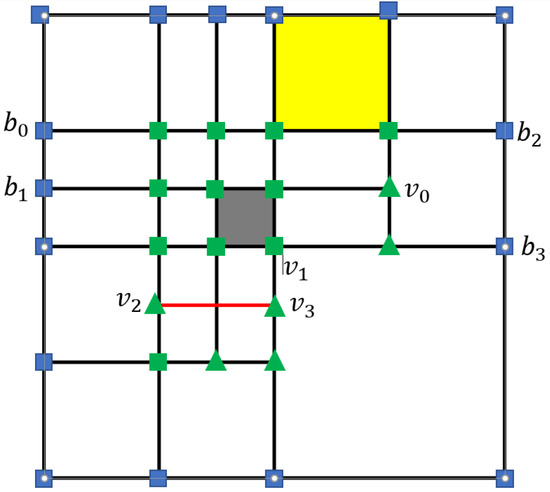
Figure 1. The vertices, edges, and cells on $\mathcal{T}$. The green square vertices denote crossing vertices, the green triangular vertices denote T-junctions.The gray cell denotes an interior cell, the yellow cell denotes a boundary cell.

We refer to a grid point in $\mathcal{T}$ as a vertex of $\mathcal{T}$. A vertex is referred to as a boundary vertex if it occupies the boundary grid line of $\mathcal{T}$; otherwise, it is referred to as an interior vertex. For example, the blue square vertices denote boundary vertices, the green square vertices, and the green triangular vertices denote interior vertices. For the interior vertices, if the valence of an interior vertex is four, it is referred to as a crossing vertex; if the valence of an interior vertex is three, it is referred to as a T-junction. For example, the green square vertices denote crossing vertices, and the green triangular vertices denote T-junctions.

We refer to the line segment that connects two adjacent vertices on one grid line as an edge of $\mathcal{T}$. An edge is referred to as a boundary edge if it occupies on the boundary of $\mathcal{T}$; otherwise, it is referred to as an interior edge. For example, $b_0{b}_1$ denotes a boundary edge, $b_1{v}_0$ denotes an interior edge. We refer to the edge as an l-edge if it is the longest possible line segment and its endpoints are either boundary vertices or T-junctions. For example, $b_1{v}_0$ and $b_0{b}_2$ denote l-edges. We refer to the interior l-edge as a T-l edge [36] if its two endpoints are both T-junctions; for example, the red segment $v_2{v}_3$ denotes a T-l-edge. Additionally, we refer to an edge as a c-edge if it is the longest possible line segment and its inner vertices are all T-junctions; for example, $v_1{b}_3$ denotes a c-edge.

We refer to each rectangular grid element as a cell of $\mathcal{T}$. A cell is referred to as an interior cell if all its edges are interior edges; otherwise, it is referred to as a boundary cell. For example, the gray cell denotes an interior cell, and the yellow cell denotes a boundary cell.

2.2. Modified Hierarchical T-Meshes

The modified hierarchical T-meshes can be defined in a recursive manner [31], which is similar to the hierarchical T-meshes in [24]. ${\mathcal{T}}^k$ denotes the mesh at level k, ${\mathcal{F}}_k$ denotes the set consist of all the cells at level k, and the set consists of the cells that are chosen to be subdivided, denoted as ${\mathsf{\Theta }}_k$, and ${\mathsf{\Theta }}_k\subset {\mathcal{F}}_k$.

• Start with a tensor product mesh ${\mathcal{T}}^0$.
• Recursive steps: Subdivide each cell in ${\mathsf{\Theta }}_k$ into $2\times 2$ equal subcells or two equal subcells to obtain a new T-mesh ${\mathcal{T}}^{k+1},k=0,1,\dots ,N.$ ${\mathcal{F}}_{k+1}$ denotes the set that consists of all current cells that emerge at level $k+1$ after subdivision.
• $\mathcal{T}={\mathcal{T}}^{N+1}$.

Figure 2 illustrates the refinement process of a modified hierarchical T-mesh dynamically.

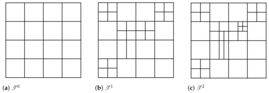
Figure 2. An example for the refinement process of a modified hierarchical T-mesh.

2.3. Spline Spaces over T-Meshes

Given a T-mesh $\mathcal{T}$, all of the cells in $\mathcal{T}$ are denoted as $\mathcal{F}$, and the region occupied by the cells in $\mathcal{T}$ is denoted as $\Omega$. The spline spaces can be defined as [23]

$$\mathbf{S}(m,n,\alpha ,\beta ,\mathcal{T}):=\{f(x,y)\in C^{\alpha ,\beta }(\Omega ):f(x,y){|}_{\varphi }\in {\mathbb{P}}_{mn},\forall \varphi \in \mathcal{F}\}.$$

(1)

Here, ${\mathbb{P}}_{mn}$ denotes the polynomial space with bi-degree $(m,n)$, and $C^{\alpha ,\beta }$ denotes the space consisting of all of the bivariate functions. These functions are $\alpha$ order-continuous in the x-direction and $\beta$ order-continuous in the y-direction on $\Omega$. Obviously, $\mathbf{S}(m,n,\alpha ,\beta ,\mathcal{T})$ should be a linear space.

In [32], the spline spaces over $\mathcal{T}$ with homogeneous boundary conditions corresponding to $\mathbf{S}(m,n,\alpha ,\beta ,\mathcal{T})$ have been defined as

$$\overline{\mathbf{S}}(m,n,\alpha ,\beta ,\mathcal{T}):=\{f(x,y)\in C^{\alpha ,\beta }\left({\mathbb{R}}^2\right):f(x,y){|}_{\varphi }\in {\mathbb{P}}_{22},\forall \varphi \in \mathcal{F},\mathrm{and}f{|}_{{\mathbb{R}}^2\backslash \Omega }\equiv 0\}.$$

(2)

As the extended T-mesh [32] will play an important role in our study, we repeat the definition of the extended T-mesh as follows.

Definition 1.

For the T-mesh$\mathcal{T}$associated with$\mathbf{S}(m,n,\alpha ,\beta ,\mathcal{T})$, the extended T-mesh can be generated in the following manner.

1. 

Add m edges to the horizontal boundaries in an average manner; add n edges to the vertical boundaries in an average manner.

2. 

Connect the boundary vertices on$\mathcal{T}$to the outer layer edges.

We denote the extended T-mesh of $\mathcal{T}$ associated with $\mathbf{S}(m,n,\alpha ,\beta ,\mathcal{T})$ as ${\mathcal{T}}^{\epsilon }$ for convenience.

Figure 3 shows a T-mesh $\mathcal{T}$, and its extended T-mesh ${\mathcal{T}}^{\epsilon }$ that associates with $\mathbf{S}(2,2,1,1,$$\mathcal{T})$. Ref. [32] gives Theorem 1 to illustrate that the spline space $\mathbf{S}(m,n,\alpha ,\beta ,\mathcal{T})$ is related to $\overline{\mathbf{S}}(m,n,\alpha ,\beta ,{\mathcal{T}}^{\epsilon })$ closely.

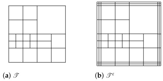
Figure 3. A T-mesh $\mathcal{T}$ and its extended T-mesh ${\mathcal{T}}^{\epsilon }$ associated with $\mathbf{S}(2,2,1,1,\mathcal{T})$.

Theorem 1

([32]). Given a T-mesh $\mathcal{T}$, ${\mathcal{T}}^{\epsilon }$ denotes the extended T-mesh associated with $\mathbf{S}(m,n,\alpha ,\beta ,$$\mathcal{T})$, and Ω denotes the region occupied by all cells of $\mathcal{T}$. Then,

$$\mathbf{S}(m,n,\alpha ,\beta ,\mathcal{T})=\overline{\mathbf{S}}(m,n,\alpha ,\beta ,{\mathcal{T}}^{\epsilon }){|}_{\Omega },$$

(3)

$$dim\mathbf{S}(m,n,\alpha ,\beta ,\mathcal{T})=dim\overline{\mathbf{S}}(m,n,\alpha ,\beta ,{\mathcal{T}}^{\epsilon }).$$

(4)

In this paper, we will discuss the subdivision rules and the basis modification framework of $\overline{\mathbf{S}}(m,n,\alpha ,\beta ,{\mathcal{T}}^{\epsilon })$ instead of $\mathbf{S}(m,n,\alpha ,\beta ,\mathcal{T})$, and then use Theorem 1 to obtain the corresponding results of $\mathbf{S}(m,n,\alpha ,\beta ,\mathcal{T})$.

3. The Space Mapping Method over the Modified Hierarchical T-Meshes

The space mapping method has been proposed in [35], which gives the conclusion that the biquadratic polynomial spline spaces over the hierarchical T-mesh is isomorphic to the piecewise constant space over the corresponding CVR graph. The bijective mapping in [35] has been used to provide a basis construction method for biquadratic polynomial spline spaces over hierarchical T-meshes. In this part, we discuss the space-mapping method over the modified hierarchical T-meshes as follows.

3.1. CVR Graph of Modified Hierarchical T-Meshes

Because the CVR graph [32,35] is critical in the space-mapping method, it can be defined in a similar manner to that of modified hierarchical T-meshes as follows.

Definition 2

([32,35]). Given a modified hierarchical T-mesh $\mathcal{T}$, the CVR graph of $\mathcal{T}$ can be constructed in the following manner.

1. 

Retain the crossing vertices and the line segments with two endpoints that are crossing vertices.

2. 

Remove the other edges and vertices from$\mathcal{T}$.

We denote the CVR graph of $\mathcal{T}$ as $\mathcal{G}$ for convenience.

Figure 4 shows an example of a CVR graph. The hierarchical T-mesh can be generated by adding some T-l edges to a modified hierarchical T-mesh, and a T-l edge on hierarchical T-mesh decays to a point on the corresponding CVR graph. Similar to [35], the notations of modified hierarchical T-meshes and the corresponding CVR graph can be defined in Table 1.

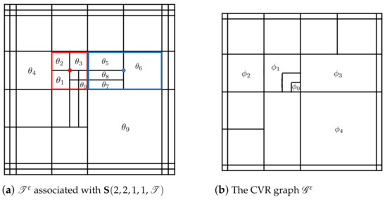
Figure 4. An example of the modified hierarchical T-mesh and its CVR graph. “•” denotes the domain-center of T-rectangle domain in the red box; “•” denotes the the domain-centre of the T-rectangle domain in the green box.

Table 1. Some notations for modified hierarchical T-meshes and the corresponding CVR graphs [35].

Notations	Abbreviations	Definitions
Modified hierarchical T-meshes:
P-cell	$\mathcal{PC}$	Four corner vertices of the cell $\theta$ are all crossing vertices or boundary vertices, $\theta$ is called a P-cell.
T-cell	-	At least one of the four corner vertices of the cell $\theta$ is a T-junction, $\theta$ is called a T-cell.
T-connected	-	If two T-cells have one common T-junction, they are called T-connected.
T-connection	$\mathcal{TC}$	The union that every two cells are T-connected.
P-domain	$\mathcal{PD}$	The domain that is occupied by a pure cell.
T-connection domain	-	The domain that is occupied by a T-connection.
T-rectangle domain	$\mathcal{TRD}$	The minimal rectangular domain that occupies on a T-connection.
Domain	$\mathcal{D}$	Each T-rectangle-domain or P-domain.
Domain-center	-	The center of the domain.
one-neighbor cell	-	For all the cells that are adjacent to the T-connection, the cells with the lowest level are called the one-neighbor cell of the T-connection.
The level of the T-connection	-	The level of the one-neighbor cells that belong to the T-connection.
CVR graph of modified hierarchical T-meshes:
g-cell	-	Each cell of the CVR graph.
P-g-cell	$\mathcal{PGC}$	Each g-cell that corresponds to a P-cell in $\mathcal{T}$.
T-g-cell	$\mathcal{TGC}$	Each g-cell that corresponds to a T-connection-domain in $\mathcal{T}$.

For example, in Figure 4a, ${\theta }_0,{\theta }_4,{\theta }_9$ we denote P-cells. The P-g cell ${\varphi }_0$ in Figure 4b corresponds to ${\theta }_0$ in Figure 4a, the P-g-cell ${\varphi }_2$ in Figure 4b corresponds to ${\theta }_4$ in Figure 4a, and the P-g-cell ${\varphi }_4$ in Figure 4b corresponds to ${\theta }_9$ in Figure 4a. ${\theta }_1,{\theta }_2,{\theta }_3,{\theta }_5,{\theta }_6,{\theta }_7, \mathrm{and} {\theta }_8$ in Figure 4a denote T-cells. The T-connection that consists of ${\theta }_1,{\theta }_2$, and ${\theta }_3$ is denoted as ${\mathcal{TC}}_0$, the minimal domain that occupies on ${\mathcal{TC}}_0$ is the T-connection domain of ${\mathcal{TC}}_0$, in Figure 4a. The domain surrounded by the red line is denoted as the T-rectangle domain of ${\mathcal{TC}}_0$, which is denoted as ${\mathcal{TRD}}_0$. ${\theta }_4$ denotes the one-neighbor cell of ${\mathcal{TC}}_0$, the level of ${\mathcal{TC}}_0$ is also the level of ${\theta }_4$, and the T-g-cell ${\varphi }_1$ in Figure 4b corresponds to the T-connection domain of ${\mathcal{TC}}_0$. The T-connection that consists of ${\theta }_5,{\theta }_6,{\theta }_7$, and ${\theta }_8$ is denoted as ${\mathcal{TC}}_1$, and the minimal domain that occupies ${\mathcal{TC}}_1$ is the T-connection domain of ${\mathcal{TC}}_1$. In Figure 4a, the domain surrounded by the blue square is denoted as the T-rectangle domain of ${\mathcal{TC}}_1$. ${\theta }_9$ denotes the one-neighbor cell of ${\mathcal{TC}}_1$, the level of ${\mathcal{TC}}_1$ is also the level of ${\theta }_9$, and the T-g-cell ${\varphi }_3$ in Figure 4b corresponds to the T-connection domain of ${\mathcal{TC}}_1$.

3.2. The Isomorphic Property

In [36,37], the dimensions of T-l edges are proposed as follows.

Theorem 2.

For a T-l edge $E\in \mathcal{T}$, if E only contains $V_0$ interior crossing vertices, then,

$$dimW\left[E\right]={(V_0-2-1)}_{+}:=max(0,V_0-2-1)$$

(5)

holds for $\mathbf{S}(2,2,1,1,\mathcal{T})$.

In particular, for the $\mathbf{S}(2,2,1,1,\mathcal{T})$, if $V_0=1$, then $dimW\left[E\right]={(V_0-d-1)}_{+}:=max(0,1-2-1)=0$, and the trivial l-edges [36,37] can be defined as follows.

Definition 3

([35]). If there exists only one crossing vertex on the T-l edge $E\in \mathcal{T}$, E is defined as a trivial l-edge associated with $\mathbf{S}(2,2,1,1,\mathcal{T})$.

For the hierarchical T-mesh $\mathcal{T}$, $\mathcal{G}$ denotes the CVR graph of $\mathcal{T}$, there exists a bijective mapping between $\mathbf{S}(2,2,1,1,\mathcal{T})$ and $\mathbf{S}(0,0,-1,-1,\mathcal{G})$, and the two spaces are isomorphic [35]:

$$\mathbf{S}(2,2,1,1,\mathcal{T})\cong \mathbf{S}(0,0,-1,-1,\mathcal{G}).$$

(6)

For a modified hierarchical T-mesh, ${\mathsf{\Theta }}_k$ denotes the subdivided cells whose levels are k first, for each cell $\theta \in {\mathsf{\Theta }}_k$, there are three different subdivision types that tend to choose [31].

• If $\theta$ is subdivided into two equal, vertically adjacent subcells, the subdivision type of $\theta$ is denoted as V.
• If $\theta$ is subdivided into two equal, horizontally adjacent subcells, the subdivision type of $\theta$ is denoted as H.
• If $\theta$ is subdivided into $2\times 2$ equal subcells, the subdivision type of $\theta$ is denoted as C.

To avoid the trivial l-edges, we can consider our subdivision rules on a modified hierarchical T-mesh as follows.

3.3. Mesh Refinement Rules

Because the subdivision scheme for modified hierarchical T-meshes can avoid the trivial l-edges that appear in hierarchical T-meshes, in this section we give our mesh refinement rules for modified hierarchical T-meshes.

To make use of the subdivision scheme of the modified hierarchical T-meshes, we use Figure 5 to illustrate the mesh refinement rules on a part of modified hierarchical T-mesh ${\mathcal{T}}_k$.

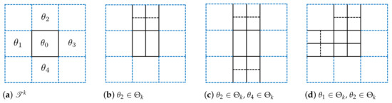
Figure 5. Mesh-refinement rules.

In Figure 5a, for ${\theta }_0\in {\mathsf{\Theta }}_k$, ${\theta }_i,i=1,\dots ,4$ are the cells around ${\theta }_0$. The refinement rules on ${\theta }_0$ can be discussed as follows.

• If ${\theta }_2\in {\mathsf{\Theta }}_k$ and the subdivision type of ${\theta }_2$ is C or V, then the subdivision type of ${\theta }_0$ is V. Figure 5b shows the refinement example.
• If ${\theta }_i\in {\mathsf{\Theta }}_k$ and the subdivision type of ${\theta }_i$ is C or V, $i=2,4$, then the subdivision type of ${\theta }_0$ is V.
• If ${\theta }_1\in {\mathsf{\Theta }}_k$ and ${\theta }_2\in {\mathsf{\Theta }}_k$, the subdivision type of ${\theta }_1$ is C or H, the subdivision type of ${\theta }_2$ is C or V, and then the subdivision type of ${\theta }_0$ is C.

If the position of ${\theta }_i,i=1,2,3,4$ is changed, the refinement rules on ${\theta }_0$ can be obtained similarly.

As a modified hierarchical T-mesh can be converted to a hierarchical T-mesh by adding corresponding trivial l-edges, we give Lemma 1 to illustrate the effection of trivial l-edges on the CVR graph.

Lemma 1.

Assume that $\mathcal{T}$ is a hierarchical T-mesh, $\mathcal{G}$ denotes the CVR graph of $\mathcal{T}$, the trivial l-edges of $\mathcal{T}$ corresponds to the vertex that is on the hanging edges of $\mathcal{G}$.

Proof of Lemma 1.

We use proof by contradiction to prove this lemma. Suppose that E is an arbitrary trivial l-edge in $\mathcal{T}$, E corresponds to the vertex V in $\mathcal{G}$, the edge which V occupies on is denoted as L. We assume that L is not the hanging edge of $\mathcal{G}$, and then v occupies the edge of a g-cell of $\mathcal{G}$. Then, there are at least two crossing vertices on E. As E is a trivial l-edge of $\mathcal{T}$, for the spline space $\mathbf{S}(2,2,1,1,\mathcal{T})$, E only contains one interior crossing vertex, this contradicts the assumption. Thus, L is a hanging edge of $\mathcal{G}$. The lemma is proven. □

For each trivial l-edge $E\in \mathcal{T}$, as $dimW\left[E\right]=0$, E is useless for $\mathbf{S}(2,2,1,1,\mathcal{T})$, from Lemma 1, E corresponds to a vertex on the hanging edge of $\mathcal{G}$. We can conclude similarly as in Equation (6) via the relationship between the CVR graph of the hierarchical T-mesh and the CVR graph of its corresponding modified hierarchical T-mesh. Our study continues here, and we can give the proof as follows.

Theorem 3.

Given a modified hierarchical T-mesh $\mathcal{T}$, assume that $\mathcal{G}$ is the corresponding CVR graph of $\mathcal{T}$, then,

$$\mathbf{S}(2,2,1,1,\mathcal{T})\cong \mathbf{S}(0,0,-1,-1,\mathcal{G}).$$

(7)

Proof of Theorem 3.

Assume that ${\mathcal{T}}_a$ is denoted as the hierarchical T-mesh and corresponds to $\mathcal{T}$ by adding the trivial l-edges $E_i,i=0,\dots ,L$, ${\mathcal{G}}_a$ is denoted as the CVR graph of ${\mathcal{T}}_a$. Then,

$$\mathbf{S}(2,2,1,1,{\mathcal{T}}_a)\cong \mathbf{S}(0,0,-1,-1,{\mathcal{G}}_a),$$

(8)

and each basis function of $\mathbf{S}(2,2,1,1,{\mathcal{T}}_a)$ corresponds to a basis function of $\mathbf{S}(0,0,-1,-1,$${\mathcal{G}}_a)$ [35]. For each trivial l-edge $E\in {\mathcal{T}}_a$, $dimW\left[E\right]=0$; thus, each basis function of $\mathbf{S}(2,2,1,1,{\mathcal{T}}_a)$ is the same with the corresponding basis function of $\mathbf{S}(2,2,1,1,\mathcal{T})$. From Lemma 1, E corresponds to the vertex that is on the hanging edges of $\mathcal{G}$, in other words, the cells of $\mathcal{G}$ are the same with the cells of ${\mathcal{G}}_a$, and each basis function of $\mathbf{S}(0,0,-1,-1,{\mathcal{G}}_a)$ is the same with the corresponding basis function of $\mathbf{S}(0,0,-1,-1,\mathcal{G})$. Thus, each basis function of $\mathbf{S}(2,2,1,1,\mathcal{T})$ corresponds to a basis function of $\mathbf{S}(0,0,-1,-1,\mathcal{G})$,

$$\mathbf{S}(2,2,1,1,\mathcal{T})\cong \mathbf{S}(0,0,-1,-1,\mathcal{G}).$$

The theorem is proven. □

From Theorem 3, we conclude that the trivial l-edges do not contribute anything useful to the mapping; hence, the bijective mapping can be described similar to that of [35] in the following manner.

For convenience, we denote $\mathbf{S}(2,2,1,1,\mathcal{T})$ as ${\mathbf{S}}^2\left(\mathcal{T}\right)$ in the following part of this paper.

3.4. The Mapping

Definition 4

([35]). Given $f(x,y)\in {\overline{\mathbf{S}}}^2\left(\mathcal{T}\right)$, and $\mathcal{D}:=[x_0,x_1]\times [y_0,y_1]$ is a rectangular domain. Let $u=\frac{x-x_0}{x_1-x_0},v=\frac{y-y_0}{y_1-y_0}$, $f(x,y)$ can be expressed as

$$f(x,y)=\sum _{j=0}^2\sum _{k=0}^2{b}_{j,k}{B}_j^2\left(u\right)B_k^2\left(v\right),$$

where $B_j^2\left(u\right)$ and $B_k^2\left(v\right)$ are Bernstein polynomials, we obtain

$$\begin{gathered} f(x,y)=b_{1,1}+\sum _{j=0}^2(b_{j,0}-b_{1,1})B_j^2\left(u\right)B_0^2\left(v\right)+\sum _{j=0,j\ne 1}^2(b_{j,1}-b_{1,1})B_j^2\left(u\right)B_1^2\left(v\right) \\ +\sum _{j=0}^2(b_{j,2}-b_{1,1})B_j^2\left(u\right)B_2^2\left(v\right). \end{gathered}$$

A mapping functional ϕ can be defined as

$$\varphi (f(x,y):\mathcal{D})=b_{1,1}{|}_{\mathcal{D}}.$$

Here, $b_{1,1}{|}_D$ denotes the piecewise constant function with value $b_{1,1}$ on $\mathcal{D}$.

Given $f(x,y)\in {\overline{\mathbf{S}}}^2\left(\mathcal{T}\right)$, $Sup\left(f\right)$ denotes the support of $f(x,y)$, we recall the notations and abbreviations in Table 1 as follows: $\mathcal{PC}$ denotes a P-cell of $Sup\left(f\right)$, $\mathcal{PD}$ denotes the P-domain of $\mathcal{PC}$, $\mathcal{PGC}$ denotes the P-g cell that corresponds to $\mathcal{PC}$ in $\mathcal{G}$, $\mathcal{TC}$ denotes a T-connection of $Sup\left(f\right)$, $\mathcal{TRD}$ denotes the T-rectangle domain of $\mathcal{TC}$, and $\mathcal{TGC}$ denotes the T-g cell corresponding to $\mathcal{TC}$ in $\mathcal{G}$. The mapping between ${\overline{\mathbf{S}}}^2\left(\mathcal{T}\right)$ and ${\overline{\mathbf{S}}}^0\left(\mathcal{G}\right)$ can be defined in the following manner.

Definition 5

([35]). The mapping between ${\overline{\mathbf{S}}}^2\left(\mathcal{T}\right)$ and ${\overline{\mathbf{S}}}^0\left(\mathcal{G}\right)$ can be defined as

$$\Phi :{\overline{\mathbf{S}}}^2\left(\mathcal{T}\right)\to {\overline{\mathbf{S}}}^0\left(\mathcal{G}\right),$$

(9)

$$\left\{\begin{array}{c}\varphi (f(x,y){|}_{\mathcal{PC}}:\mathcal{PD}){\to g(x,y)|}_{\mathcal{PGC}}\hfill \\ \varphi (f(x,y){|}_{\mathcal{TC}}:\mathcal{TRD}){\to g(x,y)|}_{\mathcal{TGC}},\hfill \end{array}\right.$$

(10)

where $f(x,y)\in {\overline{\mathbf{S}}}^2\left(\mathcal{T}\right)$, ${f(x,y)|}_{\mathcal{PC}}$ denotes the representation of $f(x,y)$ on $\mathcal{PC}$, $g(x,y)\in {\overline{\mathbf{S}}}^0\left(\mathcal{G}\right)$, and ${g(x,y)|}_{\mathcal{PGC}}$ denotes the representation of $g(x,y)$ on $\mathcal{PGC}$, and $\mathcal{PGC}$ corresponds to $\mathcal{PC}$, ${f(x,y)|}_{\mathcal{TC}}$ denotes the representation of $f(x,y)$ on the one-neighbor cell of $\mathcal{TC}$, and ${g(x,y)|}_{\mathcal{TGC}}$ denotes the representation of $g(x,y)$ on $\mathcal{TGC}$, and $\mathcal{TGC}$ corresponds to $\mathcal{TC}$.

To illustrate the mapping, we give an example from ${\overline{\mathbf{S}}}^2\left(\mathcal{T}\right)$ to ${\overline{\mathbf{S}}}^0\left(\mathcal{G}\right)$ as follows.

Example 1.

We present the mapping example for both P-g cells and T-g cells separately because the CVR graph only contains the two types of cells.

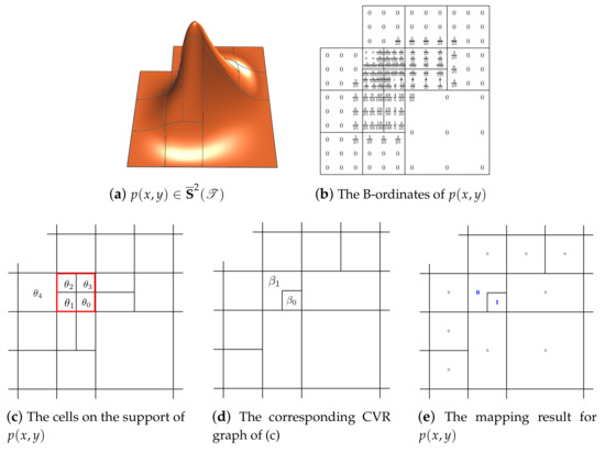
For $p(x,y)\in {\overline{\mathbf{S}}}^2\left(\mathcal{T}\right)$ in Figure 6a, the B-ordinates on the cells belong to the support of $p(x,y)$ is shown in Figure 6b. In Figure 6c, $p(x,y)$ occupies on ${\theta }_i$ is denoted as $p{(x,y)}_i,i=0,1,\dots ,4,$ respectively. ${\beta }_0$ is a P-cell in $\mathcal{T}$, $\mathcal{PD}$ denotes the P-domain of ${\theta }_0$. The T-connection $\mathcal{TC}$ is constituted of ${\theta }_1,{\theta }_2, and {\theta }_3$. $\mathcal{TRD}$ denotes the T-rectangle domain of $\mathcal{TC}$. As the P-g cell ${\beta }_0$ in Figure 6d corresponds to the P-cell ${\theta }_0$ in Figure 6c, from Definition 5, we obtain

$$\varphi (p_0(x,y):\mathcal{PD}){\to 1|}_{{\beta }_0}.$$

Figure 6. A mapping example from ${\overline{\mathbf{S}}}^2\left(\mathcal{T}\right)$ to ${\overline{\mathbf{S}}}^0\left(\mathcal{G}\right)$. The red box in (c) denotes the T-rectangle domain. 0 and 1 in (e) denote the values on the corresponding g-cells.

As the T-g cell ${\beta }_1$ in Figure 6d corresponds to the T-connection domain of $\mathcal{TC}$ in Figure 6c and ${\theta }_4$ is the one-neighbor cell of $\mathcal{TC}$, from Definition 5, we obtain

$$\varphi (p_4(x,y):\mathcal{TRD}){\to 0|}_{{\beta }_1}.$$

Similarly, we can obtain the mapping results for the other cells on the support of $p(x,y)$. Figure 6d shows the whole mapping result.

3.5. The Inverse Mapping (Basis Function Construction Process)

From Theorem 3, we can construct the basis function by the basis construction process in [35]. ${\mathcal{T}}^k$ denotes the modified hierarchical T-mesh at level k, and ${\mathcal{G}}^k$ denotes the CVR graph of ${\mathcal{T}}^k$. We describe the construction process of a basis function $b_j^{k+1}(x,y)\in {\overline{\mathbf{S}}}^2({\mathcal{T}}^{k+1})$ as follows.

The inverse mapping is the process for constructing $b_j^{k+1}$, the tools for evaluating B-ordinates of each basis function of ${\overline{\mathbf{S}}}^2({\mathcal{T}}^{k+1})$ are T-structures; we recall T-structures in [35] as follows.

In Figure 7, the c-edge $v_0{v}_m$ and the cells ${\theta }_0,\dots ,{\theta }_n$ constitute a T-structure, which is denoted as $\mathcal{T}$. $v_0{v}_m$ denotes the mid-edge of $\mathcal{T}$. $v_0,\dots ,v_m$ denote the interior vertices of $\mathcal{T}$. $v_0$ and $v_m$ denote the endpoints of $\mathcal{T}$. ${\theta }_0$ denotes the mother cell of $\mathcal{T}$. ${\theta }_5,\dots ,{\theta }_n$ denote the subcells of $\mathcal{T}$. ${\theta }_0$ denotes the mother cell of $\mathcal{T}$, and the level of $\mathcal{T}$ is also the level of ${\theta }_0$. Additionally, $\mathcal{T}$ should be a horizontal T-structure.

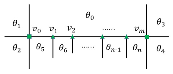
Figure 7. The T-structure ${\mathcal{T}}^{k+1}$.

For the modified hierarchical T-mesh ${\mathcal{T}}^{k+1}$, a T-structure, which is denoted as $\mathcal{T}$, consists of one c-edge $E_c$ and all the cells that have at least one common vertex with $E_c$. The interior structure of $\mathcal{T}$ is shown in Figure 7. If there is one common interior vertex of a horizontal T-structure ${\mathcal{T}}_h$ and the other vertical T-structure ${\mathcal{T}}_v$, we call ${\mathcal{T}}_h$ and ${\mathcal{T}}_v$ connected. A T-structure branch, which is denoted as $\mathcal{TSB}$, consists of the union that every two T-structures are connected. The level of $\mathcal{TSB}$ is the minimal level of all the T-structures in $\mathcal{TSB}$.

From the notations of T-structures and T-structure branches above, several algorithms in [35] are given to evaluate the B-ordinates for the T-cells of the T-connections, we recall the algorithms as follows.

Algorithm 1 illustrates the pattern to order the T-structures in a T-structure branch, Algorithm 2 describes the detailed procedures for using T-structures to calculate the B-ordinates of a T-connection. By Algorithms 1 and 2, we can give Algorithm 3 to calculate the B-ordinates for a basis function $b^{k+1}(x,y)\in {\overline{\mathbf{S}}}^2({\mathcal{T}}^{k+1})$. This is different from the method of searching the domain that supports a basis function in [35]. We can choose the support of a basis function $b^k(x,y)\in {\overline{\mathbf{S}}}^2({\mathcal{T}}^k)$ as the domain that is supports $b^{k+1}(x,y)$ directly.

Algorithm 1: Ordering the T-structures for each T-structure-Branch of ${\mathcal{T}}^{k+1}$ [35].

Algorithm 2: Evaluating the B-ordinates for each T-cell in ${\mathcal{TC}}_0\in {\mathcal{T}}^{k+1}$ [35].

Algorithm 3: Calculating the B-ordinates for $b^{k+1}(x,y)\in {\overline{\mathbf{S}}}^2\left({\mathcal{T}}^{k+1}\right)$.

Figure 8 shows the construction process for $b_j^{k+1}(x,y)\in \mathbf{S}(2,2,1,1,{\mathcal{T}}^{k+1})$. The basis construction process can be summarized as follows.

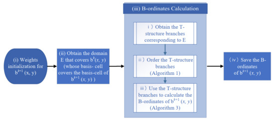
Figure 8. Process for basis construction.

• Weights initialization for $b^{k+1}(x,y)$:
  Given the basis function $q^{k+1}(x,y)\in {\overline{\mathbf{S}}}^0({\mathcal{G}}^{k+1})$ as

  $$q^{k+1}(x,y)=\left\{\begin{array}{cc}1,\hfill & \mathcal{GC}\in {\mathcal{G}}^{k+1}\hfill \\ 0,\hfill & \mathrm{other}\mathrm{g}-\mathrm{cells}\mathrm{of}{\mathcal{G}}^{k+1},\hfill \end{array}\right.$$

  (11)

  by Equation (11), the weight on the domain center can be initialized as

  $$\omega =\left\{\begin{array}{cc}1,\hfill & (\frac{x_0+x_1}{2},\frac{y_0+y_1}{2})\hfill \\ 0,\hfill & \mathrm{other}\mathrm{domain}-\mathrm{centres},\hfill \end{array}\right.$$

  (12)

  where $(\frac{x_0+x_1}{2},\frac{y_0+y_1}{2})$ denotes the domain center of $\mathcal{D}$ on ${\mathcal{T}}^{k+1}$.
• Obtain the domain $\mathbb{E}$ covers $Sup\left(b^{k+1}(x,y)\right)$.
  As the basis cell of each basis function at level $k+1$ is a part of the basis cell that belongs to a basis function at level k, the support of $b^{k+1}(x,y)$ is covered by a basis function $b^k(x,y)\in {\overline{\mathbf{S}}}^2({\mathcal{T}}^k)$, we adopt the support of $b^k(x,y)$ as $\mathbb{E}$.
• B-ordinates Calculation.

  (a)

  Obtain the T-structure-branches corresponding to $\mathbb{E}$.

  Obviously, $\mathbb{E}$ is referred to as the union of two different types of components: P-cells and T-connections. The center B-ordinate for each P-cell are obtained by Equation (12) directly. Assume there are n T-connections in $\mathbb{E}$, and they are ${\mathcal{TC}}_0,{\mathcal{TC}}_1,\dots ,{\mathcal{TC}}_n$, the T-structure-branch that covers ${\mathcal{TC}}_i$ is denoted as ${\mathcal{TSB}}_i,i=0,\dots ,n$.

  (b)

  Order the T-structure branches.

  The center B-ordinate for each cell belongs to E can be evaluated by this T-structure branches as follows. First, we sort the T-structures in each T-structure branch by Algorithm 1, and then sort all of the T-structure branches in descending level order.

  (c)

  Evaluate the B-ordinates of $b^{k+1}(x,y)$ via T-structures.

  First, we adopt Algorithm 3 for calculating the center B-ordinates on T-cells of each T-connection, and then we evaluate the B-ordinates on the rest edges that are not obtained via the $C^1$ continuous conditions.

• Save the B-ordinates in $Sup\left(b^{k+1}(x,y)\right)$.
  If there exists nonzero B-ordinates in $\theta \in \mathbb{E}$, then save the B-ordinates on $\theta$ into $Sup\left(b^{k+1}(x,y)\right)$.

We give an example to show the process for calculating the B-ordinates for a basis function $b^{k+1}(x,y)\in {\overline{\mathbf{S}}}^2({\mathcal{T}}^{k+1})$. We illustrate the above process as follows.

Example 2.

1.

Weights initialization for$b^{k+1}(x,y)$. Figure 9a shows a part of hierarchical T-mesh.Figure 9b shows the corresponding part of its CVR graph. For$q^{k+1}(x,y))\in {\overline{\mathbf{S}}}^0({\mathcal{G}}^{k+1})$, the weights of$b^{k+1}(x,y)\in {\overline{\mathbf{S}}}^2({\mathcal{T}}^{k+1})$are initialized by Equation (12), we show the initialized weights in Figure 9b.

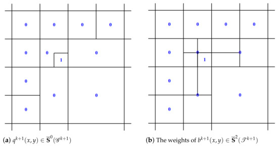Figure 9. Weights initialization. The 0 and 1 in (a) denote the value on each g-cell that belongs to a part of ${\mathcal{G}}^{k+1}$; The 0 and 1 in (b) denote the corresponding initialized weights.

2.

Obtain the domain$\mathbb{E}$covers$Sup\left(b^{k+1}(x,y)\right)$. We focus our attention on the part of the mesh that is shown inFigure 9b because the support of the basis function on the cells inFigure 9b covers$Sup\left(b^{k+1}(x,y)\right)$.

3.

B-ordinates Calculation.

(a) 

Obtain the T-structure branches corresponding to$\mathbb{E}$. InFigure 10, there are three T-structure branches:${\mathcal{TC}}_0,{\mathcal{TC}}_1,and{\mathcal{TC}}_2$. ${\mathcal{TC}}_0$is constituted of${\theta }_0,{\theta }_1$, and${\theta }_2$. ${\mathcal{TC}}_1$is constituted of${\theta }_3,{\theta }_4$, and${\theta }_5$. ${\mathcal{TC}}_1$is constituted of${\theta }_6,{\theta }_7$, and${\theta }_8$. ${\mathcal{TC}}_i$corresponds to the T-structure branch${\mathcal{TSB}}_i,i=0,1,2$. ${\mathcal{TSB}}_0$, which is the blue structure inFigure 10, is constituted of${\mathcal{T}}_0$(the c-edge$v_0{v}_2$and cells adjacent to$v_0{v}_2$) and${\mathcal{T}}_1$ (the c-edge $v_1{v}_3$ and cells adjacent to $v_1{v}_3$); ${\mathcal{TSB}}_1$, which is the yellow structure in Figure 10, is constituted of ${\mathcal{T}}_2$ (the c-edge $v_0{v}_5$ and cells adjacent to $v_0{v}_5$), and ${\mathcal{T}}_3$ (the c-edge $v_4{v}_6$ and cells adjacent to $v_4{v}_6$). ${\mathcal{TSB}}_2$, which is the green structure in Figure 10, is constituted of ${\mathcal{T}}_4$ (the c-edge $v_7{v}_8$ and cells adjacent to $v_7{v}_8$) and ${\mathcal{T}}_5$ (the c-edge $v_8{v}_9$ and cells adjacent to $v_8{v}_9$).

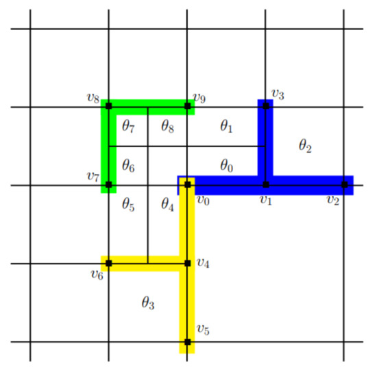Figure 10. The T-structure-branches of $\mathbb{E}$. The blue structure denotes T-structure-branch that is constituted of ${\mathcal{T}}_0$ (the c-edge $v_0{v}_2$ and cells adjacent to $v_0{v}_2$) and ${\mathcal{T}}_1$ (the c-edge $v_1{v}_3$ and cells adjacent to $v_1{v}_3$); The yellow structure denotes T-structure-branch that is constituted of ${\mathcal{T}}_2$ (the c-edge $v_0{v}_5$ and cells adjacent to $v_0{v}_5$), and ${\mathcal{T}}_3$ (the c-edge $v_4{v}_6$ and cells adjacent to $v_4{v}_6$).; The green structure denotes T-structure-branch that is constituted of ${\mathcal{T}}_4$ (the c-edge $v_7{v}_8$ and cells adjacent to $v_7{v}_8$) and ${\mathcal{T}}_5$ (the c-edge $v_8{v}_9$ and cells adjacent to $v_8{v}_9$).

(b) 

Order the T-structure branches. The level of${\mathcal{T}}_0$is lower than the level of${\mathcal{T}}_1$. Thus, we can order the T-structures in${\mathcal{TSB}}_0$as${\mathcal{T}}_0,{\mathcal{T}}_1$. Similarly, the T-structures in${\mathcal{TSB}}_1$can be ordered as${\mathcal{T}}_2,{\mathcal{T}}_3$, the T-structures in${\mathcal{TSB}}_2$can be ordered as${\mathcal{T}}_4,{\mathcal{T}}_5$.

(c) 

Evalute the B-ordinates of$b^{k+1}(x,y)$via T-structures.Figure 11shows the process of using the T-structure-branches that are ordered inFigure 3b to calculate B-ordinates of$b^{k+1}(x,y)$. Figure 12shows the rest B-ordinates obtained by the$C^1$continuous conditions.

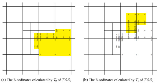
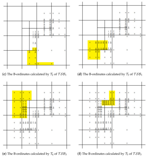Figure 11. The process of B-ordinates calculation. The values in the highlight domain are the new evaluated B-ordinates on the corresponding domain points.

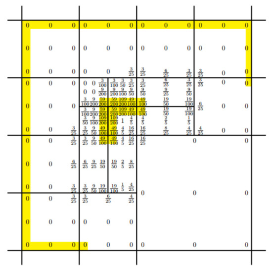Figure 12. The rest B-ordinates. The values in the highlight domain are the new evaluated B-ordinates on the corresponding domain points.

4.

Save the B-ordinates of$Sup\left(b^{k+1}(x,y)\right)$. The support of$b^{k+1}(x,y)$is the cells without the top left cell.

For the basis function whose basis cell is a P-cell, we give the construction method above.

4. Basis Construction Framework with Modifications

In fact, there are two types of basis cells for the basis functions of ${\overline{\mathbf{S}}}^2({\mathcal{T}}^{k+1})$. One corresponds to a P-cell on ${\mathcal{T}}^{k+1}$; we can construct such basis functions by the method in Section 3.5. The other corresponds to a T-connection on ${\mathcal{T}}^{k+1}$, and we discuss the modification process of such basis function in this section. In addition, we introduce the whole basis construction framework with modifications in this section.

4.1. Basis Modification Method

First, we define basis modification as follows.

Definition 6.

Given a basis function$b_i^k(x,y)$at level k, the set consists of the cells of${\mathsf{\Theta }}_k$that belongs to$Sup\left(b_i^k(x,y)\right)$as${\mathsf{\Theta }}_{k_i}$. For each cell θ of${\mathsf{\Theta }}_{k_i}$, modify$b_i^k(x,y)$from level k to level$k+1$, the modified basis function can be denoted as

$${\overline{b}}_i^k(x,y)={\mathfrak{M}}^{k+1}\left(b_i^k\right)(x,y).$$

The modification process can be described as

1. 

using 9 B-ordinates to represent$b_i^k(x,y)$over θ;

2. 

adopting de Casteljau’s algorithm for generating new B-ordinates on θ according to the different subdivision types; and

3. 

modifying the B-ordinates that are associated with${\overline{b}}_i^k(x,y)$by Algorithm 4.

Algorithm 4: Modification of ${\overline{b}}_i^k(x,y)$

To demonstrate the basis modification in Definition 6, we provide the following example.

Example 3.

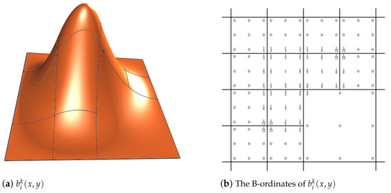
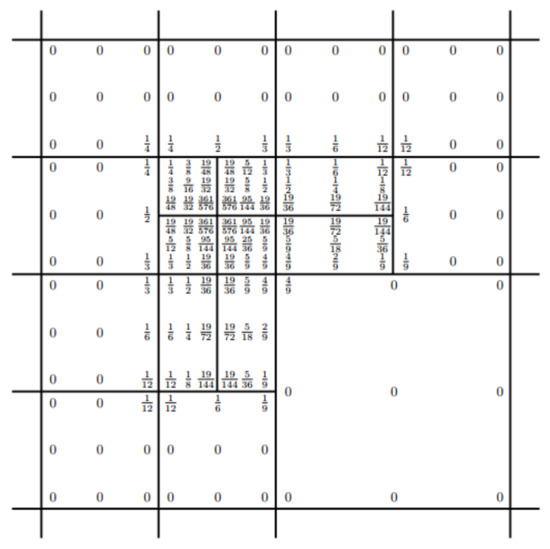
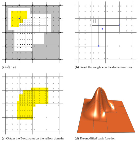
Figure 13a shows a basis function $b_i^k(x,y)\in {\overline{\mathbf{S}}}^2({\mathcal{T}}^k)$, the B-ordinates on $b_i^k(x,y)$ are shown in Figure 13b. First, refine the cells of ${\mathsf{\Theta }}_{k_i}$ according to the different subdivision type, Figure 14 shows the refined mesh. Subdivide the B-ordinates according to the different subdivision types. The B-ordinates subdivision result is also shown in Figure 14.

Figure 13. A basis function at level $k$.

Figure 14. The subdivided B-ordinates of $b_i^k(x,y)$.

In Figure 15a, the crossing vertex, which is denoted as the blue square, is subdivided. As the crossing vertex is a corner vertex of a connection, and the four edges are either the edges or the c-edges of ${\mathcal{T}}^k$, we can reserve the 16 B-ordinates around the crossing vertex. The subdivision will not influence the B-ordinates on the domain points whose B-ordinates are zero, we can reserve the B-ordinates (B-ordinates in the gray domain) on the crossing vertices in Figure 15a. Then, we need to calculate the B-ordinates on the black dots in Figure 15a. Additionally, we reset the weights on the domain centres in Figure 15b. At last, we can calculate the rest of the B-ordinates on the yellow domain in Figure 15c via Algorithm 3, the modified basis function is shown in Figure 15d. From above, we modify a basis function $b_i^k(x,y)\in {\overline{\mathbf{S}}}^2({\mathcal{T}}^k)$ to ${\overline{b}}_i^k(s,t)\in {\overline{\mathbf{S}}}^2({\mathcal{T}}^{k+1})$.

Figure 15. Basis modification. The values in the highlight domain of (a) are the reserved B-ordinates. “■” in (a) denotes the crossing vertex. 0 and 1 in (b) denotes the reset weights. The values in the highlight domain of (c) are the new evaluated B-ordinates on the domain points that corresponds to the “•” in (a).

Algorithm 4 gives the process for basis modification from ${\overline{\mathbf{S}}}^2({\mathcal{T}}^k)$ to ${\overline{\mathbf{S}}}^2({\mathcal{T}}^{k+1})$, without loss of generality. If there are more than one basis cells at level $k+1$ appearing in a basis function of ${\overline{\mathbf{S}}}^2({\mathcal{T}}^k)$, the modification will display similarly.

4.2. Basis Construction Framework

From the above, we give the basis construction and modification framework by Algorithm 5.

Algorithm 5: Basis construction and modification of ${\overline{\mathbf{S}}}^2({\mathcal{T}}^{k+1})$.

In this section, we present the algorithm for basis modification and discuss the framework for basis construction with modification.

5. Fitting Open Meshes

Surface fitting is an essential method in the field of CAD. In this section, we use several triangular surface models to show the potential of splines generated by our method.

Given the open surface model $\mathcal{M}$ in 3D space, $\mathcal{M}$ is constituted of a series of triangles, the vertices on $\mathcal{M}$ are denoted as $V_0,V_1,\dots ,V_N$, we parameterize $\mathcal{M}$ by using the parametrization method in [38]. The parameter mesh is a triangle mesh. The parameter value corresponding to $V_i$ is denoted as $V_i^{\prime }(x_i,y_i),i=0,\dots ,N$, and the parameter domain is $[0,1]\times [0,1]$. Additionally, the triangle on the parameterized mesh is denoted as $\Delta$.

5.1. Calculation of Control Points

Different from the least square optimization method in [24,31], we adopt the domain centres for calculating the control points as follows.

Given the basis functions $b_j(x,y),j=1,\dots ,m$, let $[x_{i_m},x_{i_m+1}]\times [y_{i_m},y_{i_m+1}]$ be the domain corresponding to basis cell of $b_j(x,y),j=1,\dots ,m$, and $(x_m,y_m)=(\frac{x_{i_m}+x_{i_m+1}}{2},\frac{y_{i_m}+y_{i_m+1}}{2})$ denotes the domain centre of $[x_{i_m},x_{i_m+1}]\times [y_{i_m},y_{i_m+1}]$. We calculate the control points by solving the following linear system

$$S(x_k,y_k)={V^{\prime }}_k,k=1,2,\dots ,m.$$

(13)

Here, $(x_k,y_k)\in {\Delta }_l:((x_{k_1},y_{k_1}),(x_{k_2},y_{k_2}),(x_{k_3},y_{k_3}))$, ${V^{\prime }}_k=w_{k_1}{V}_{k_1}+w_{k_2}{V}_{k_2}+w_{k_3}{V}_{k_3}$, and $w_{k_1},w_{k_2},w_{k_3}$ can be evaluated by $(x_k,y_k)=w_{k_1}(x_{k_1},y_{k_1})+w_{k_2}(x_{k_2},y_{k_2})+w_{k_3}(x_{k_3},y_{k_3})$.

5.2. Process of Fitting

With the method of calculating control points, we run the loop of steps 2, steps 3, and steps 4, until the error reaches the given tolerance $\epsilon$.

• Given the $4\times 4$ tensor-product mesh ${\mathcal{T}}^0$.
• For the old basis functions, we retain their control points; for the new basis functions of ${\mathbf{S}}^2({\mathcal{T}}^k)$, calculate their control points via Section 5.1. The result modified spline space is denoted as $S(x,y)$.
• ${\mathsf{\Theta }}_k\leftarrow \theta$, if $ma{x}_{(x,y)\in \theta }=\Vert V(x,y)-S(x,y)\Vert >\epsilon$.
• We use mesh-refinement rules in Section 3.3 to denote the cells in ${\mathsf{\Theta }}_k$. We subdivide the mesh and modify the basis functions via Algorithm 5.
  $k\leftarrow k+1$.

Figure 16, Figure 17, Figure 18 and Figure 19 illustrate four examples, in which basis functions of spline space over hierarchical T-meshes and modified hierarchical T-meshes are shown. Both basis functions over the two types of meshes provide a good approximation of the original model. However, the number of subdivided cells over modified hierarchical T-meshes are lower than that over hierarchical T-meshes at the same level. The statistical data for comparison are listed in Table 2. The comparisons for the solutions on hierarchical T-meshes and modified hierarchical T-meshes are provided in Figure 20. The comparison shows that the solution on the modified hierarchical T-meshes can achieve similar accuracy with fewer subdivision cells.

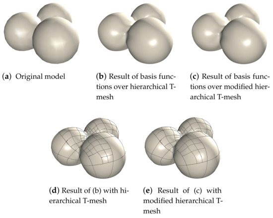
Figure 16. Balls.

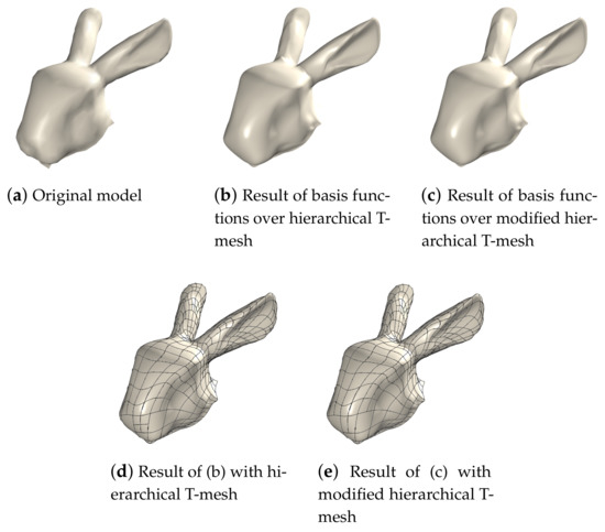
Figure 17. Bunny head.

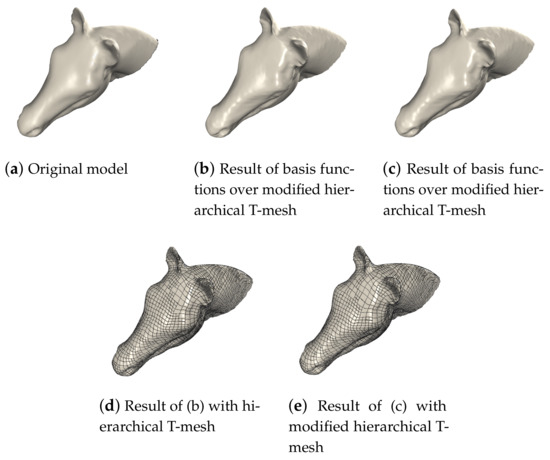
Figure 18. Horse head.

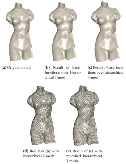
Figure 19. Venus body.

Table 2. Experiment data.

Hierarchical T-Meshes			Modified Hierarchical T-Meshes
Models	Levels	#Subdivision Cells	#Max Error	#Subdivision Cells	#Max Error
Balls	1	16	0.169909	16	0.169909
	3	144	0.0840613	139	0.0840613
	5	195	0.0550255	170	0.0550255
	7	225	0.0071944	192	0.0071944
Bunny head	1	16	0.237579	16	0.237579
	3	166	0.084061	151	0.084061
	5	358	0.161495	290	0.159583
	7	547	0.048042	433	0.048038
	9	691	0.007814	526	0.009279
Horse head	1	16	0.4413	16	0.4413
	Level 3	256	0.3082	256	0.3082
	5	1309	0.1405	1174	0.1405
	7	2380	0.0885	2148	0.0885
	9	3454	0.0295	3063	0.0295
	11	3829	0.0093	3380	0.0093
	12	3958	0.0014	3477	0.0014
Venus body	1	16	0.596	16	0.596
	3	256	0.401	256	0.401
	5	1231	0.1521	1129	0.1521
	7	1915	0.0755	1708	0.0755
	9	2830	0.0199	2501	0.0199
	11	3490	0.0064	3055	0.0064
	12	3613	0.003	3127	0.004

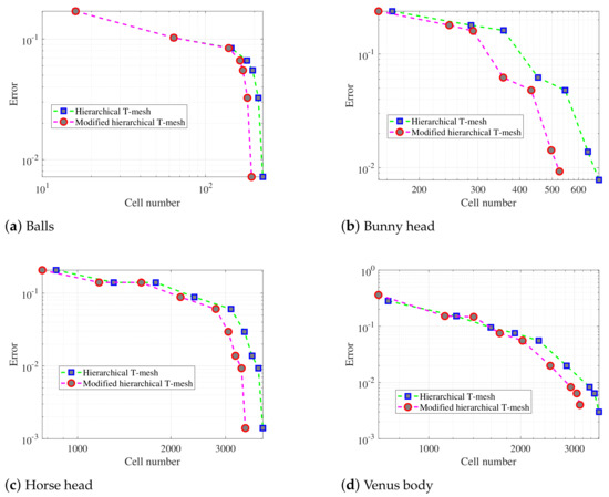
Figure 20. Convergence results of basis functions over hierarchical T-meshes and modified hierarchical T-meshes.

6. Conclusions

In this paper, we provide a unique basis construction framework that incorporates basis modification of the spline space over modified hierarchical T-meshes. The subdivision rules on the modified hierarchical T-meshes are also given to prevent the redundant edges that exist on hierarchical T-meshes. Algorithms within the framework make the construction of basis functions easy to operate. In the basis construction framework, the splines over the modified hierarchical T-mesh are modified to accommodate the insertion of the cells on the corresponding CVR graph. The modification process is driven as follows: for each cell belongs to ${\mathsf{\Theta }}_k$, it is subdivided into four subcells or two subcells on ${\mathcal{T}}^{k+1}$. For each basis function at level k, if some of the corresponding CVR cells are subdivided, the basis function will be modified as a basis function of level $k+1$. If a basis cell is generated by the subdivision process, we will reconstruct the corresponding basis function. Moreover, the application of the above splines in surface reconstruction with adaptive refinement is discussed in detail. In comparison to splines over hierarchical T-meshes, modified hierarchical T-meshes have fewer cells subdivided when achieving similar accuracy.

References

- Farin, G.; Hoschek, J.; Kim, M.S. Handbook of Computer Aided Geometric Design; Elsevier: Amsterdam, The Netherlands, 2002. [Google Scholar]
- Hughes, T.; Cottrell, J.; Bazilevs, Y. Isogeometric analysis: CAD, finite elements, NURBS, exact geometry and mesh refinement. Comput. Methods Appl. Mech. Eng. 2005, 194, 4135–4195. [Google Scholar] [CrossRef]
- Sederberg, T.W.; Zheng, J.; Bakenov, A.; Nasri, A. T-Splines and T-NURCCs. ACM Trans. Graph. 2003, 22, 477–484. [Google Scholar] [CrossRef]
- Sederberg, T.W.; Cardon, D.L.; Finnigan, G.T.; North, N.S.; Zheng, J.; Lyche, T. T-Spline Simplification and Local Refinement. ACM Trans. Graph. 2004, 23, 276–283. [Google Scholar] [CrossRef]
- Bazilevs, Y.; Calo, V.; Cottrell, J.; Evans, J.; Hughes, T.; Lipton, S.; Scott, M.; Sederberg, T. Isogeometric analysis using T-splines. Comput. Methods Appl. Mech. Eng. 2010, 199, 229–263. [Google Scholar] [CrossRef]
- Dörfel, M.R.; Jüttler, B.; Simeon, B. Adaptive isogeometric analysis by local h-refinement with T-splines. Comput. Methods Appl. Mech. Eng. 2010, 199, 264–275. [Google Scholar] [CrossRef]
- Li, X.; Zheng, J.; Sederberg, T.W.; Hughes, T.J.; Scott, M.A. On linear independence of T-spline blending functions. Comput. Aided Geom. Des. 2012, 29, 63–76. [Google Scholar] [CrossRef]
- Scott, M.; Li, X.; Sederberg, T.; Hughes, T. Local refinement of analysis-suitable T-splines. Comput. Methods Appl. Mech. Eng. 2012, 213–216, 206–222. [Google Scholar] [CrossRef]
- Li, X.; Zhang, J. AS++ T-splines: Linear independence and approximation. Comput. Methods Appl. Mech. Eng. 2018, 333, 462–474. [Google Scholar] [CrossRef]
- Forsey, D.R.; Bartels, R.H. Hierarchical B-Spline Refinement. In Proceedings of the 15th Annual Conference on Computer Graphics and Interactive Techniques, SIGGRAPH ’88, Atlanta, GA, USA, 1–5 August 1988; pp. 205–212. [Google Scholar]
- Unther Greiner, G.; Hormann, K. Interpolating and Approximating Scattered 3D-Data with Hierarchical Tensor Product B-Splines; Vanderbilt University Press: Nashville, TN, USA, 1997; pp. 163–172. [Google Scholar]
- Schillinger, D.; Dedè, L.; Scott, M.A.; Evans, J.A.; Borden, M.J.; Rank, E.; Hughes, T.J. An isogeometric design-through-analysis methodology based on adaptive hierarchical refinement of NURBS, immersed boundary methods, and T-spline CAD surfaces. Comput. Methods Appl. Mech. Eng. 2012, 249–252, 116–150. [Google Scholar] [CrossRef]
- Vuong, A.V.; Giannelli, C.; Jüttler, B.; Simeon, B. A hierarchical approach to adaptive local refinement in isogeometric analysis. Comput. Methods Appl. Mech. Eng. 2011, 200, 3554–3567. [Google Scholar] [CrossRef]
- Evans, E.; Scott, M.; Li, X.; Thomas, D. Hierarchical T-splines: Analysis-suitability, Bézier extraction, and application as an adaptive basis for isogeometric analysis. Comput. Methods Appl. Mech. Eng. 2015, 284, 1–20. [Google Scholar] [CrossRef]
- Giannelli, C.; Jüttler, B.; Speleers, H. THB-splines: The truncated basis for hierarchical splines. Comput. Aided Geom. Des. 2012, 29, 485–498. [Google Scholar] [CrossRef]
- Giannelli, C.; Jüttler, B.; Speleers, H. Strongly stable bases for adaptively refined multilevel spline spaces. Adv. Comput. Math. 2014, 40, 459–490. [Google Scholar] [CrossRef]
- Giannelli, C.; Jüttler, B.; Kleiss, S.K.; Mantzaflaris, A.; Simeon, B.; Špeh, J. THB-splines: An effective mathematical technology for adaptive refinement in geometric design and isogeometric analysis. Comput. Methods Appl. Mech. Eng. 2016, 299, 337–365. [Google Scholar] [CrossRef]
- Kiss, G.; Giannelli, C.; Zore, U.; Jüttler, B.; Großmann, D.; Barner, J. Adaptive CAD model (re-)construction with THB-splines. Graph. Model. 2014, 76, 273–288. [Google Scholar] [CrossRef]
- Speleers, H.; Manni, C. Effortless quasi-interpolation in hierarchical spaces. Numer. Math. 2016, 132, 155–184. [Google Scholar] [CrossRef]
- Dokken, T.; Lyche, T.; Pettersen, K.F. Polynomial splines over locally refined box-partitions. Comput. Aided Geom. Des. 2013, 30, 331–356. [Google Scholar] [CrossRef]
- Bressan, A.; Jüttler, B. A hierarchical construction of LR meshes in 2D. Comput. Aided Geom. Des. 2015, 37, 9–24. [Google Scholar] [CrossRef]
- Bressan, A. Some properties of LR-splines. Comput. Aided Geom. Des. 2013, 30, 778–794. [Google Scholar] [CrossRef]
- Deng, J.; Chen, F.; Feng, Y. Dimensions of spline spaces over T-meshes. J. Comput. Appl. Math. 2006, 194, 267–283. [Google Scholar] [CrossRef]
- Deng, J.; Chen, F.; Li, X.; Hu, C.; Tong, W.; Yang, Z.; Feng, Y. Polynomial splines over hierarchical T-meshes. Graph. Model. 2008, 70, 76–86. [Google Scholar] [CrossRef]
- Li, X.; Deng, J.; Chen, F. Surface modeling with polynomial splines over hierarchical T-meshes. Vis. Comput. 2007, 23, 1027–1033. [Google Scholar] [CrossRef]
- Wang, J.; Yang, Z.; Jin, L.; Deng, J.; Chen, F. Adaptive surface reconstruction based on implicit PHT-splines. In Proceedings of the 14th ACM Symposium on Solid and Physical Modeling, Haifa, Israel, 1–3 September 2010; pp. 101–110. [Google Scholar]
- Tian, L.; Chen, F.; Du, Q. Adaptive finite element methods for elliptic equations over hierarchical T-meshes. J. Comput. Appl. Math. 2011, 236, 878–891. [Google Scholar] [CrossRef]
- Nguyen-Thanh, N.; Nguyen-Xuan, H.; Bordas, S.P.A.; Rabczuk, T. Isogeometric analysis using polynomial splines over hierarchical T-meshes for two-dimensional elastic solids. Comput. Methods Appl. Mech. Eng. 2011, 200, 1892–1908. [Google Scholar] [CrossRef]
- Nguyen-Thanh, N.; Kiendl, J.; Nguyen-Xuan, H.; Wüchner, R.; Bletzinger, K.U.; Bazilevs, Y.; Rabczuk, T. Rotation free isogeometric thin shell analysis using PHT-splines. Comput. Methods Appl. Mech. Eng. 2011, 200, 3410–3424. [Google Scholar] [CrossRef]
- Wang, P.; Xu, J.; Deng, J.; Chen, F. Adaptive isogeometric analysis using rational PHT-splines. Comput.-Aided Des. 2011, 43, 1438–1448. [Google Scholar] [CrossRef]
- Ni, Q.; Wang, X.; Deng, J. Modified PHT-splines. Comput. Aided Geom. Des. 2019, 73, 37–53. [Google Scholar] [CrossRef]
- Deng, J.; Chen, F.; Jin, L. Dimensions of biquadratic spline spaces over T-meshes. J. Comput. Appl. Math. 2013, 238, 68–94. [Google Scholar] [CrossRef]
- Deng, F.; Zeng, C.; Wu, M.; Deng, J. Bases of Biquadratic Polynomial Spline Spaces over Hierarchical T-Meshes. J. Comput. Math. 2017, 35, 91–120. [Google Scholar] [CrossRef]
- Zeng, C.; Deng, F.; Deng, J. Bicubic hierarchical B-splines: Dimensions, completeness, and bases. Comput. Aided Geom. Des. 2015, 38, 1–23. [Google Scholar] [CrossRef]
- Liu, J.; Deng, F.; Deng, J. Space Mapping of Spline Spaces over Hierarchical T-meshes. arXiv 2022, arXiv:2103.11688. [Google Scholar] [CrossRef]
- Zeng, C.; Deng, F.; Li, X.; Deng, J. Dimensions of biquadratic and bicubic spline spaces over hierarchical T-meshes. J. Comput. Appl. Math. 2015, 287, 162–178. [Google Scholar] [CrossRef]
- Wu, M.; Deng, J.; Chen, F. Dimension of spline spaces with highest order smoothness over hierarchical T-meshes. Comput. Aided Geom. Des. 2013, 30, 20–34. [Google Scholar] [CrossRef]
- Floater, M.S. Parametrization and smooth approximation of surface triangulations. Comput. Aided Geom. Des. 1997, 14, 231–250. [Google Scholar] [CrossRef]
Publisher’s Note: MDPI stays neutral with regard to jurisdictional claims in published maps and institutional affiliations. |
© 2022 by the authors. Licensee MDPI, Basel, Switzerland. This article is an open access article distributed under the terms and conditions of the Creative Commons Attribution (CC BY) license (https://creativecommons.org/licenses/by/4.0/).