The Modified Local Boundary Knots Method for Solution of the Two-Dimensional Advection–Diffusion Equation

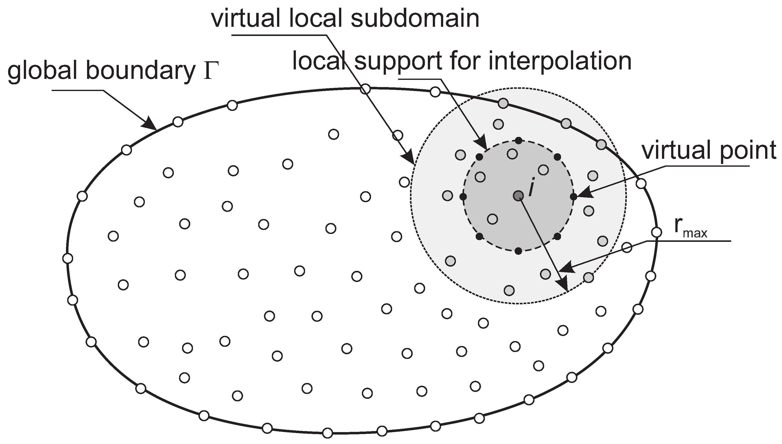
Abstract

This paper deals with a new modification of the local boundary knots method (LBKM), which will allow the irregular node distribution and the arbitrary shape of the solution domain. Unlike previous localizations, it has no requirements on the number of nodes in the support or on the number of virtual points. Owing to the limited number of virtual points, the condition number of boundary knots matrix remains relatively low. The article contains the derivation of the relations of the method for steady and unsteady states and shows its effectiveness in three control examples.

1. Introduction

In recent decades, the significant evolution of meshless methods for solving partial differential equations is evident. The first sign of this trend can be considered the boundary element method (BEM) [1,2], which is not yet an utterly network-free method. However, it has significantly reduced the necessary network of elements. On the other hand, this method required solving the integrals of the fundamental solution, which was sometimes very complicated. The removal of integration is the main advantage of the method of fundamental solution (MFS) [3,4,5], which uses fundamental solutions as basis functions to approximate the solution without needing integration. This property has contributed to the significant expansion of this method and its considerable popularity. However, this method also has its problems, especially related to using a network of fictitious virtual points. The singular boundary method (SBM) [6,7,8] tries to eliminate this disadvantage using real points at the boundary of an area to be identified with fictitious points. At the same time, however, this leads to the need to solve the problems of the singularity of the fundamental solution in case the two points are identical. SBM solves this by introducing the so-called origin intensity factors (OIF) [6,9], which are calculated in a more or less complicated way and are essentially the main weakness of this method. Another way to solve the singularity uses the boundary knot method (BKM) [10,11,12], which uses the general solution of the governing differential equation as the basis function instead of the fundamental solution.

Unfortunately, the condition number of the BKM interpolation matrix is very high, and its inversion is overburdensome. Recently, a local BKM solution [13,14] can help keep the interpolation matrix conditional on a reasonable level, thus enabling even more extensive tasks. Nevertheless, even so, with more local support, problems can arise. These should be removed by the presented modification of the local BKM. It is based partly on the LBIEM principle [15,16] and separates the virtual area around each point from its support. It allows keeping the condition number of the matrix independent of the number of points in the support.

Our article focuses on the solution of the steady and non-steady advection–diffusion problem, which is of great practical importance, e.g., in modeling the transport of substances in a flowing liquid. The first two sections describe the connection between BKM and FC and its application to the advection–diffusion problem in the two-dimensional domain. The following sections present the control examples and compare the results with the exact solution.

2. Governing Equations

The governing equation of the unsteady hydrodynamic dispersion in the domain $\mathsf{\Omega }\in {\mathbb{R}}_2$ with boundary $\mathsf{\Gamma }$ is

$$R_d\frac{\partial C(\mathbf{x},t)}{\partial t}=D\mathsf{\Delta }C(\mathbf{x},t)-\mathbf{v}·\nabla C(\mathbf{x},t)-\lambda C(\mathbf{x},t)\mathbf{x}\in \mathsf{\Omega },$$

(1)

where C is the concentration of the tracer, D is the coefficient of dispersion, $R_d$ is the retardation factor, $\lambda$ is the decay coefficient, $\mathbf{x}$ are spatial coordinates, v is the vector of velocity, and t is the time.

The usual boundary conditions of Equation (1) are as follows:

-

The Dirichlet boundary conditions, where the value of the concentration C on the part of boundary ${\mathsf{\Gamma }}_1$ is prescribed, i.e., $C=C_0(\mathbf{x},t)$$\mathbf{x}\in {\mathsf{\Gamma }}_1$;

-

The Neumann boundary conditions, where the flux $q_0$ with concentration $C_0$ perpendicular to the boundary ${\mathsf{\Gamma }}_2$ is given, i.e.,

$$D\frac{\partial C}{\partial x_i}{n}_i=(C-C_0)q_0(\mathbf{x},t)\mathbf{x}\in {\mathsf{\Gamma }}_2,$$

(2)

where $n_i$ is the i component of the outer normal vector, perpendicular to the boundary ${\mathsf{\Gamma }}_2$.

These are in addition to the whole boundary $\mathsf{\Gamma }={\mathsf{\Gamma }}_1\cup {\mathsf{\Gamma }}_2$. The initial condition is defined by the prescribed value of the concentration at time $t_0=0$.

All boundary conditions can be simply expressed as

$$\mathcal{B}\left(u\right)=b_0(\mathbf{x},t)\mathbf{x}\in \mathsf{\Gamma },$$

(3)

where $\mathcal{B}\left(u\right)$ is the boundary operator.

3. Numerical Solution

Time-dependent tasks are solved in two main ways when using meshless methods. We can use a time-dependent fundamental or general solution of a differential equation, or approximate the time term using a finite difference (FD) scheme. Since the time-dependent general solution of the advection–diffusion equation is difficult to find, we replaced the time derivative on the left side of (1) with a finite difference scheme.

The backward (Euler) scheme (4) is the simplest and can be defined as

$$\frac{\partial C^{n+1}}{\partial t}=\frac{1}{\mathsf{\Delta }t}\left(C^{n+1}-C^n\right).$$

(4)

When we applied the scheme (4) to the presented method, it performed poorly for long time series. Therefore, we are looking for a more suitable and accurate scheme.

The Houbolt method [8,17] is an implicit and unconditionally stable FD scheme that can be obtained by the cubic-Lagrange interpolation of the concentration C from time $(n-2)\mathsf{\Delta }t$ through to time $(n+1)\mathsf{\Delta }t$. This scheme can be written as

$$\frac{\partial C^{n+1}}{\partial t}=\frac{1}{6\mathsf{\Delta }t}\left(11C^{n+1}-18C^n+9C^{n-1}-2C^{n-2}\right),$$

(5)

where $\mathsf{\Delta }t$ is the time step and the superscripts n − 2, n − 1, n, and n + 1 of u represent the time level. The differential Equation (1) is now changed to

$$D\mathsf{\Delta }{C}^{n+1}-\mathbf{v}·\nabla C^{n+1}-\lambda C^{n+1}=\frac{R_d}{6\mathsf{\Delta }t}\left(11C^{n+1}-18C^n+9C^{n-1}-2C^{n-2}\right).$$

(6)

The simple Euler formula is used in the first two steps to obtain the needed data $C^n$ and $C^{n-1}$ to start the Houboldt scheme ($C^{n-2}$ is a given initial solution).

To solve the unsteady diffusion Equation (1), we represent the solution as a sum of homogeneous and particular solutions. The solution of (6) can now be defined as the sum

$$C^{n+1}=C_H^{n+1}+C_P^{n+1},$$

(7)

where $C_H^{n+1}$ is a solution of homogeneous differential equation in time level $n+1$ that satisfies boundary conditions and $C_P^{n+1}$ is a particular solution of the non-homogeneous Equation (6). The homogeneous problem has been solved using the modified local boundary knots method (LBKM). The particular solution could be solved using the local method of approximating particular solutions (LMAPS) [9,18].

3.1. Homogeneous Solution

As is usual with most local methods, we assume that the domain $\mathsf{\Omega }$ is covered by individual points. We find a group of the nearest points for each point $i\in \mathsf{\Omega }$ that form the support. In this modified version, in addition to support, we need to define a circular virtual area around each point and regularly spaced virtual points at its boundary (Figure 1). In this area, we now approximate the value of the concentration at a given point i and time interval n + 1 using the general solution of a homogeneous differential equation in the form

$$C{\left(x_i\right)}_H^{n+1}=\sum _{j=1}^n{\alpha }_j{G}^{*}\left(r_{ij}\right)x_i\in \mathsf{\Omega },$$

(8)

where n is the number of virtual points, $r_{ij}=∥{\mathbf{x}}_i-{\mathbf{x}}_j∥$ is the distance between point i and virtual point j, and $G^{*}$ is the general solution. For the 2D advection–diffusion differential Equation (6), the non-singular general solution is given as

$$G^{*}\left(r_{ij}\right)=\frac{1}{2\pi }exp\left(\frac{\mathbf{v}·\mathbf{r}}{2D}\right)I_0\left(\mu r_{ij}\right),$$

(9)

where $r_{ij}=∥x_i-x_j∥$, $I_0$ is the modified Bessel function of the first kind and

$$\mu =\sqrt{{\left(\frac{\left.∥\mathbf{v}\right|}{2D}\right)}^2+\frac{\lambda }{D}}.$$

(10)

Figure 1. Virtual and supporting nodes in the domain $\mathsf{\Omega }$.

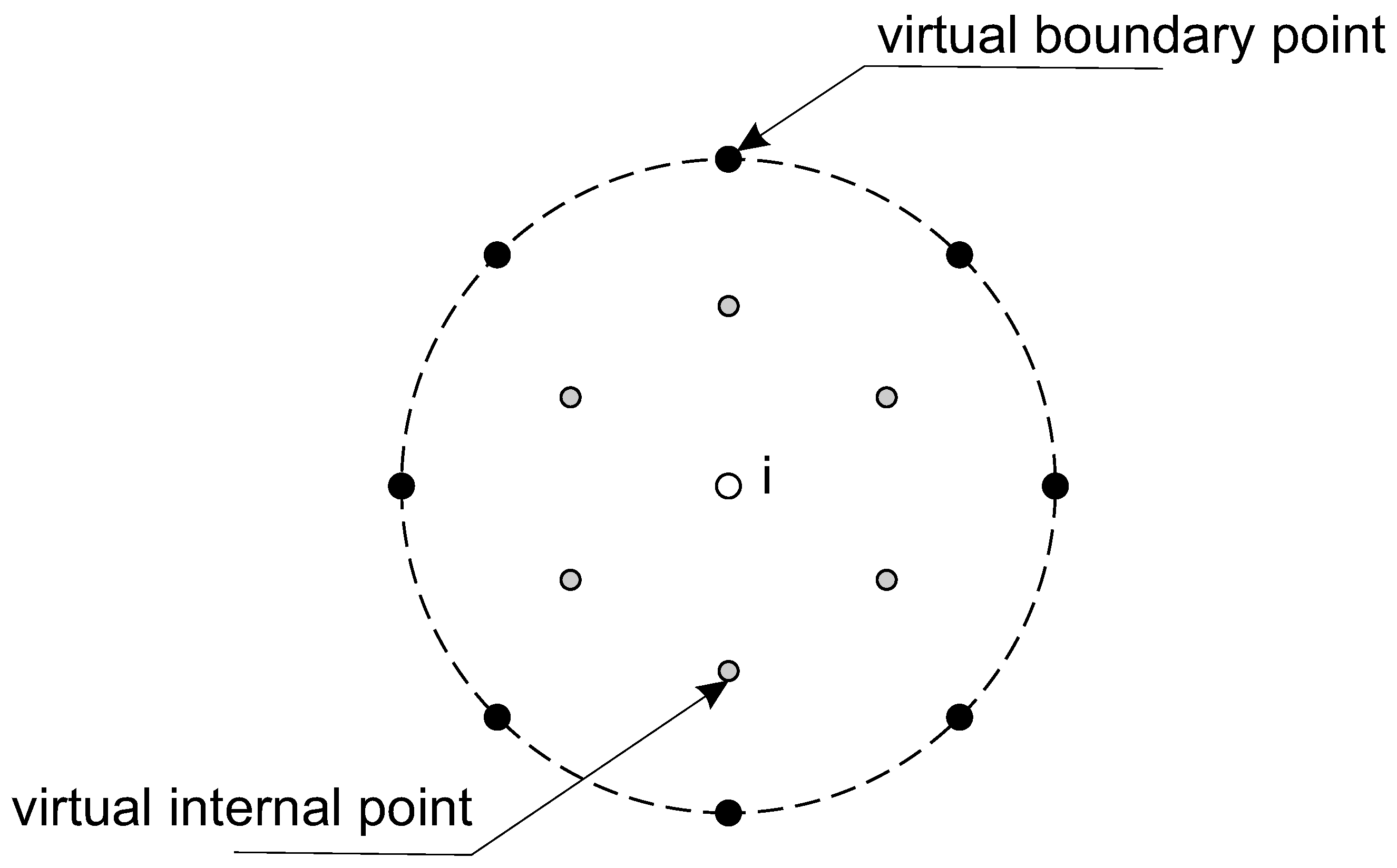
The coefficients ${\alpha }_j$ are unknown and we determine them by applying (8) to all virtual points and we obtain

$$\sum _{j=1}^n{A}_{kj}{\alpha }_j=C_{k}k=1\dots n,$$

(11)

where $C_k$ are the values of concentrations in virtual points for homogeneous solution.

3.2. Particular Solution

The particular solution $C_P^{n+1}$ is approximated by radial basis (RBF) functions as

$$C_P^{n+1}=\sum _{j=1}^p{\beta }_j^{n+1}\mathsf{\Theta }\left(r_j\right),$$

(12)

where $\mathsf{\Theta }\left(r_j\right)$ are radial basis functions, ${\beta }_j^{n+1}$ are unknown coefficients, and p is the number of internal virtual points in the virtual subdomain of the point i. These points can be regularly placed inside the subdomain (see Figure 2). The function $\mathsf{\Theta }$ is defined as a solution of the following equation [2,8]

$$D\mathsf{\Delta }\mathsf{\Theta }\left(r_j\right)-\mathbf{v}·\nabla \mathsf{\Theta }\left(r_j\right)-\lambda \mathsf{\Theta }\left(r_j\right)=\phi \left(r_j\right),$$

(13)

where $\phi \left(r_j\right)$ are also the radial basis functions. There are various possibilities for how to choose these functions [2,19]. Instead of choosing the simple form of the function $\phi \left(r_j\right)$ on the right-hand side of (13), we choose the simple expression for the basis functions $\mathsf{\Theta }\left(r_j\right)$. By substituting into (13), we can obtain the corresponding formula for the function $\phi \left(r_j\right)$. In our paper, we chose $\mathsf{\Theta }\left(r_j\right)$ functions as multiquadrics (MQ) and we obtain

$$\begin{array}{c}\hfill \mathsf{\Theta }\left(r\right)=\sqrt{r^2+R_P^2}\hfill \\ \hfill \phi \left(r\right)=D\frac{r^2+2R_P^2}{{\left(r^2+R_P^2\right)}^{3/2}}-\frac{\mathbf{r}·\mathbf{v}}{\sqrt{r^2+R_P^2}}-\lambda \sqrt{r^2+R_P^2},\hfill \end{array}$$

(14)

where $R_P$ is the shape factor of the particular solution. This factor can be different from the factor R used in (21). According to (6) and (13), we can write

$$\sum _{j=1}^p{\beta }_j^{n+1}\phi \left(r_j\right)=R_d\frac{11\left(C_P^{n+1}+C_H^{n+1}\right)-18C^n+9C^{n-1}-2C^{n-2}}{6\mathsf{\Delta }t}.$$

(15)

Figure 2. Virtual subdomain around the node i.

Matrix A from Equation (11) is now extended to $(n+p)\times (n+p)$ dimension and it has the following structure

$$\mathbf{A}=\left[\begin{array}{cc}\mathbf{K}& \mathbf{L}\\ \mathbf{M}& \mathbf{N}\end{array}\right],$$

(16)

where

$$\begin{array}{cc}\hfill K_{kj}=G^{*}\left(r_{kj}\right)\hfill & \hfill k,j=1\dots n\hfill \\ \hfill L_{kl}=\mathsf{\Theta }\left(r_{kl}\right)\hfill & \hfill l=1\dots p\hfill \end{array}$$

(17)

in the boundary virtual points (see Figure 2) and

$$\begin{array}{cc}\hfill M_{lj}=-\frac{11R_d}{6\mathsf{\Delta }t}{G}^{*}\left(r_{lj}\right)\hfill & \hfill l=1\dots p,j=1\dots n\hfill \\ \hfill N_{lq}=\phi \left(r_{lq}\right)-\frac{11R_d}{6\mathsf{\Delta }t}\mathsf{\Theta }\left(r_{lq}\right)\hfill & \hfill l,q=1\dots p\hfill \end{array}$$

(18)

in the internal virtual points (see Figure 2). For the first two time intervals, when we use the Euler scheme, Formula (18) has the form

$$\begin{array}{cc}\hfill M_{lj}=-\frac{R_d}{\mathsf{\Delta }t}{G}^{*}\left(r_{lj}\right)\hfill & \hfill l=1\dots p,j=1\dots n\hfill \\ \hfill N_{lq}=\phi \left(r_{lq}\right)-\frac{R_d}{\mathsf{\Delta }t}\mathsf{\Theta }\left(r_{lq}\right)\hfill & \hfill l,q=1\dots p\hfill \end{array}$$

(19)

Since the virtual points do not correspond to the nodes in the support, we must express $C_k$ as a function of the concentrations in the support using some interpolation method. In our article, we have chosen the combination of the weighted radial basis functions and polynomials.

The unknown values $C_k$ in virtual source points are approximated in a support of the point i as

$$C_k=\sum _{l=1}^m{\beta }_l^k\mathcal{R}\left(r_{kl}\right)+\sum _{l=1}^M{\chi }_l^k{p}_l(x_k,y_k),k=1\dots n,$$

(20)

where ${\beta }_l^k$ and ${\chi }_l^k$ are the weights, $\mathcal{R}\left(r_{kl}\right)$ are the radial basis functions, and $p_l$ are polynomials with degree M-1. M is the order of $\mathcal{R}$, and m is the number of nodes in the support of a reference point. In our paper, the multiquadrics functions [19] have been used

$$\mathcal{R}\left(r_{kl}\right)=\sqrt{R^2+r_{kl}^2},$$

(21)

where R is a so-called shape factor of the multiquadric function. We can determine the weighting coefficients ${\beta }_j^k$ and ${\chi }_j^k$ in Equation (20) by requiring that this equation is fulfilled at all m support points. Then, by the procedure described, e.g., in [20], we obtain a set of RBF shape functions ${\mathsf{\Phi }}_l^k$ and we can write

$$C_k=\sum _{l=1}^m{\mathsf{\Phi }}_l^k{C}_l.$$

(22)

Now, we can substitute (22) to the right side of (11) and obtain

$$\sum _{j=1}^n{A}_{kj}{\alpha }_j=\sum _{l=1}^m{\mathsf{\Phi }}_l^k{C}_{l}k=1\dots n$$

(23)

in matrix notation

$$\mathbf{A}\mathsf{\alpha }=\mathsf{\Phi }\mathbf{C}$$

(24)

and we can obtain the unknown coefficients ${\alpha }_j$ as

$$\mathsf{\alpha }={\mathbf{A}}^{-1}\mathsf{\Phi }\mathbf{C}.$$

(25)

For a homogeneous (steady) solution without internal virtual points, matrix A has dimensions $(n\times n)$ and matrix $\mathsf{\Phi }(n\times m)$. The concentration in point i can now be expressed as

$$C_i={\mathbf{G}}_i^T\mathsf{\alpha }={\mathbf{G}}_i^T{\mathbf{A}}^{-1}\mathsf{\Phi }\mathbf{C}={\mathbf{W}}_i^T\mathbf{C},$$

(26)

where ${\mathbf{W}}^i$ is a weight vector of the point i [21]. The vector W can be used to assemble the global system of equations to solve homogeneous problems. This system is sparse and can be defined as

$$\begin{array}{cc}\hfill C_i=C_{0i}& \forall i\in {\mathsf{\Gamma }}_1\\ \hfill C_i-\sum _{j=1}^m{W}_j^i{u}_j=0& \forall i\in \mathsf{\Omega }\\ \hfill \sum _{j=1}^m\frac{\partial W_j^i}{\partial \mathbf{n}}{u}_j=q_{0i}{C}_{0i}& \forall i\in {\mathsf{\Gamma }}_2,\end{array}$$

(27)

where m is the number of points in the i-th support.

For a non-stationary problem, it is necessary to add a particular solution (see Section 3.2), and we must extend the matrices A and $\mathsf{\Phi }$ to the dimensions $(n+p)\times (n+p)$ and $(n+p)\times m$, respectively. Then, (26) remains formally the same but the weight vector W also consists of two parts

$${\mathbf{W}}^i=\left\{\begin{array}{cc}{\mathbf{W}}_1^i& {\mathbf{W}}_2^i\end{array}\right\}.$$

(28)

The resulting system of sparse linear equations in the time $t^{n+1}$ can be written as

$$\begin{array}{cc}\hfill C_i^{n+1}=C_{0i}\hfill & \hfill \forall i\in {\mathsf{\Gamma }}_1\hfill \\ \hfill C_i^{n+1}-\sum _{j=1}^m{W}_{1j}^i{C}_j^{n+1}=-\frac{R_d}{6\mathsf{\Delta }t}\sum _{j=1}^p{W}_{2j}^i\left(18C_j^n-9C^{n-1}+2C^{n-2}\right)\hfill & \hfill \forall i\in \mathsf{\Omega }\hfill \\ \hfill \sum _{j=1}^m\frac{\partial W_{1j}^i}{\partial \mathbf{n}}{C}_j^{n+1}=q_{0i}(C_i^n-C_{0i})\hfill & \hfill \forall i\in {\mathsf{\Gamma }}_2.\hfill \end{array}$$

(29)

We can solve these N equations to obtain values of concentration at all nodes in n + 1 time step.

In the case of the steady problem, the algorithm of the method can be clearly described by the following steps:

• We define the support of each point in the area.
• We generate virtual points around each point.
• We prepare RBF shape functions ${\Phi }$ according to (22).
• We calculate the matrix A according to (11) for each point, except for the points where the Dirichlet boundary condition is prescribed.
• At these points, we solve the system of linear Equation (26) and obtain the weight vector W.
• We use this weight vector to construct a sparse global matrix of linear equations according to (27).
• We multiply the prescribed values of the Dirichlet boundary condition by the corresponding values of the weight vector W and, thus, create the right side.
• By solving the equations, we obtain the concentration values at the points of the area.

The following style will modify the algorithm, describing the unsteady state: The first three steps will be the same as in the steady problem, and we start with step No. 4.

4.

We generate internal virtual points.

5.

We calculate the matrix A according to (19) for each point, except for the points where the Dirichlet boundary condition is prescribed.

6.

At these points, we solve the system of linear Equation (26) and obtain the weight vector W.

7.

We use this weight vector to construct a sparse global matrix of linear equations according to (29).

8.

We use the initial conditions and create the right side of the global system (29).

9.

We multiply the prescribed values of the Dirichlet boundary condition by the corresponding values of the weight vector W and add the results to the right side.

10.

By solving the global equations, we obtain the concentration values at the points of the area in the next time step.

11.

We can use the results and change the right side of the global system.

12.

We repeat steps No. 9 to 11 in the first two time steps.

13.

We calculate the new matrix A according to (18) and reassemble the global system of equations.

14.

We prepare the system’s right side using all previous values of concentrations.

15.

By solving the global equations, we obtain the concentration values at the points of the area in the next time step.

16.

We repeat steps No. 14 to 15 in all remaining time steps.

4. Results

To test the possibilities of the proposed method, we present the results of several test examples in this chapter. In all these cases, the exact analytical solution is known; therefore, it is possible to compare the error of the numerical method. The root mean squared error (RMSE) and $R_{\infty }$ are employed to evaluate accuracy. These errors are defined as

$$RMSE=\sqrt{\frac{{\sum }_{i=1}^N{({\overline{C}}_i-C_i)}^2}{N}}{R}_{\infty }=\underset{i=1...N}{max}\left(\right|{\overline{C}}_i-C_i\left|\right),$$

(30)

where ${\overline{C}}_i$ is the exact value of concentration in point i.

When solving advection–diffusion problems, the Peclet number Pe is often used to assess the effect of advection

$$Pe=\frac{∥\mathbf{v}∥L}{D}.$$

(31)

All examples have been computed on a PC computer with an Intel(R) Core(M) i7-8550U processor (1.8 GHz CPU), a 64-bit Windows 11 operating system, and a 16 GB internal memory. The programming language has been Visual C++ and Eigen library for sparse matrix operations.

4.1. Example No. 1, Steady Case

In the first example, we consider the steady advection–diffusion problem with the Dirichlet boundary conditions [22]. The domain is a unit square with prescribed concentrations

$$\begin{array}{c}\hfill C(x,0)=\frac{1-e^{(x-1)v_x/D}}{1-e^{-v_x/D}}\end{array}$$

(32)

$$\begin{array}{c}\hfill C(0,y)=\frac{1-e^{(y-1)v_y/D}}{1-e^{-v_y/D}}.\end{array}$$

(33)

The dispersion coefficient is $D=1$ and the velocity vector is $\mathbf{v}=(v_x,v_y)$ and $v_x=v_y$. The exact solution to this problem is [22]

$$C(x,y)=\frac{\left(1-e^{(x-1)v_x/D}\right)\left(1-e^{(y-1)v_y/D}\right)}{\left(1-e^{-v_x/D}\right)\left(1-e^{-v_y/D}\right)}.$$

(34)

For the numerical solution of this example, three meshes were used. Two meshes were regular with 21 × 21 and 51 × 51 points. The third mesh was irregular with 5426 points. This example was solved with three different Peclet numbers, namely, Pe = 10, 30, and 50. Table 1 shows the solution RMSEs for all previously mentioned meshes and three different Peclet numbers.

Table 1. Example No. 1—comparison of RMSE and $R_{\infty }$ for different meshes and Pe values.

Pe	Mesh $21\times 21$		Mesh $51\times 51$		Irregular Mesh
	RMSE	${\mathit{R}}_{\mathit{\infty }}$	RMSE	${\mathit{R}}_{\mathit{\infty }}$	RMSE	${\mathit{R}}_{\mathit{\infty }}$
10	9.1395$\times {10}^{-4}$	2.7817$\times {10}^{-3}$	1.4861$\times {10}^{-4}$	4.4874$\times {10}^{-4}$	9.5202$\times {10}^{-5}$	4.0198$\times {10}^{-4}$
30	6.0220$\times {10}^{-3}$	3.5671$\times {10}^{-2}$	9.3171$\times {10}^{-4}$	4.6437$\times {10}^{-3}$	7.3789$\times {10}^{-4}$	5.1634$\times {10}^{-3}$
50	1.3147$\times {10}^{-2}$	9.4959$\times {10}^{-2}$	2.1142$\times {10}^{-3}$	1.3600$\times {10}^{-2}$	1.8039$\times {10}^{-3}$	2.0027$\times {10}^{-2}$

The course of the absolute error in the profile x = y is also interesting (Figure 3). It is clear that for higher Peclet numbers, the most significant error is concentrated in the largest concentration gradient at the upper right corner of the area. In Figure 4, we can see the contours of the absolute error of the solution for a regular network of 51 × 51 points and a Peclet number of 10 and 30.

Figure 3. Example No. 1—irregular mesh, absolute errors in the profile x = y.

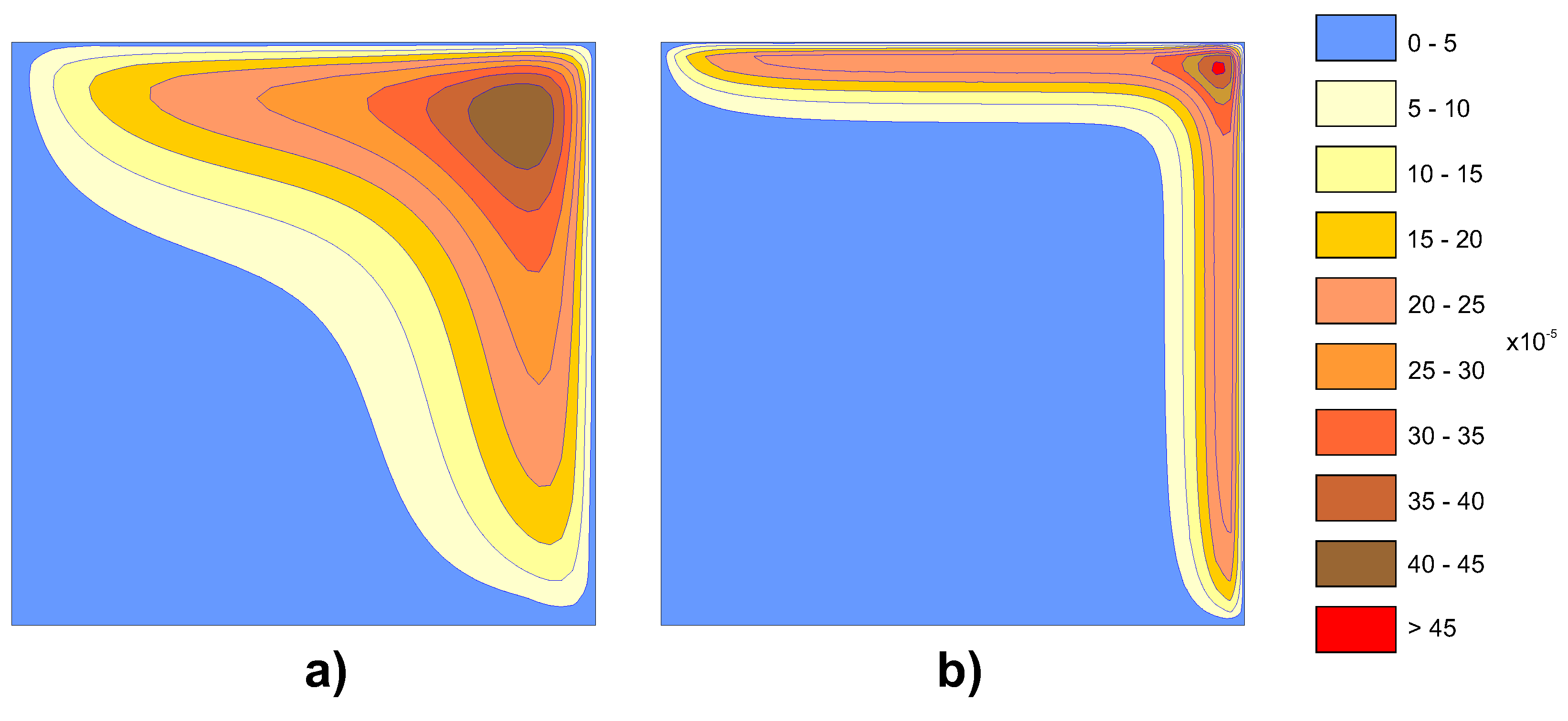
Figure 4. Example No. 1—contours of absolute errors, (a) Pe = 10, (b) Pe = 30.

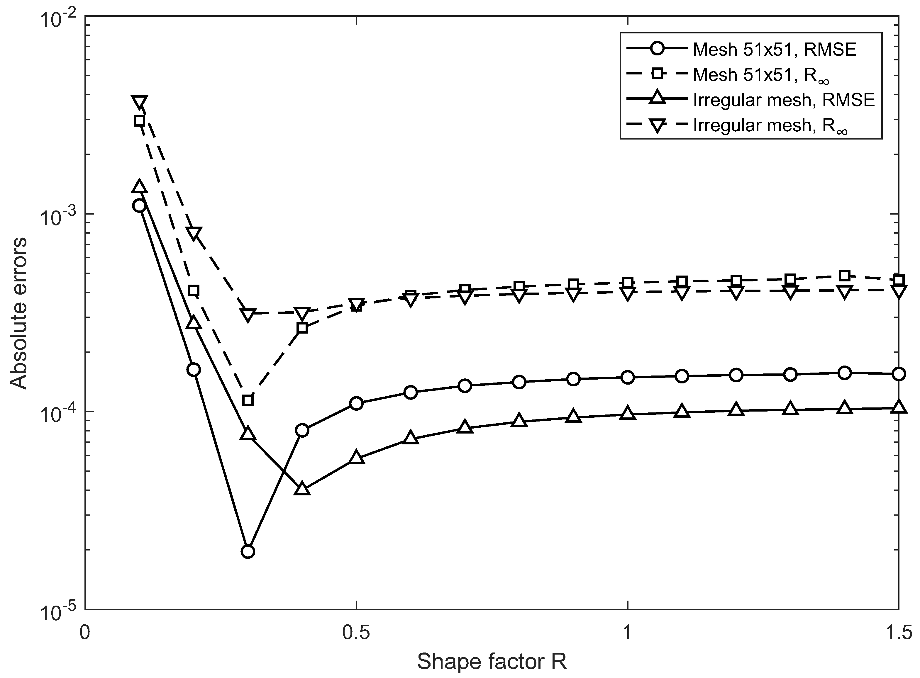
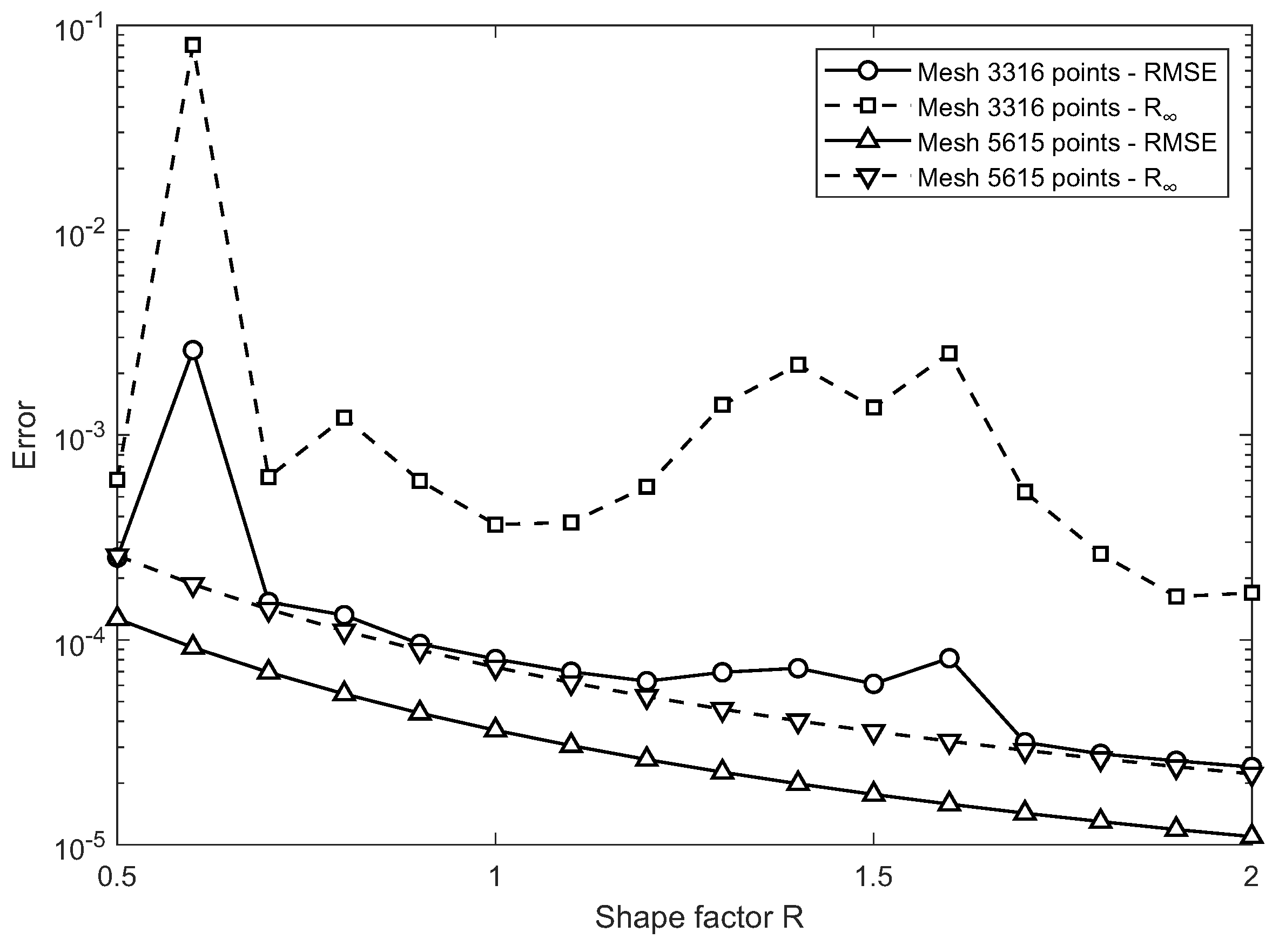
In this example, we also tested the effect of the number of virtual points n and support points m on the method’s accuracy. It has been shown that increasing the number of virtual points does not lead linearly to reducing errors (Table 2).

Table 2. Example No. 1—comparison of RMSE and $R_{\infty }$ for different number of virtual points.

n	Regular Mesh 51 × 51		Irregular Mesh
	RMSE	${\mathit{R}}_{\mathit{\infty }}$	RMSE	${\mathit{R}}_{\mathit{\infty }}$
6	1.4862$\times {10}^{-4}$	4.4850$\times {10}^{-4}$	9.6585$\times {10}^{-5}$	4.0193$\times {10}^{-4}$
8	1.4861$\times {10}^{-4}$	4.4789$\times {10}^{-4}$	9.6592$\times {10}^{-5}$	4.0197$\times {10}^{-4}$
12	1.4783$\times {10}^{-4}$	4.4629$\times {10}^{-4}$	9.6779$\times {10}^{-5}$	4.0168$\times {10}^{-4}$
16	1.4884$\times {10}^{-4}$	4.4984$\times {10}^{-4}$	9.6639$\times {10}^{-5}$	4.0198$\times {10}^{-4}$

As for supporting points, point i itself has been also included in the support. The shape of the support for a regular network has been a square with sides formed by an odd number of points. For an irregular network, the algorithm described in [23] has been used. The principle is to divide the vicinity of point i into identical segments, and the point in the segment closest to point i is taken into support.

As seen from Table 3, there is a certain optimal number of points in the support, and further increasing the number of points will not cause an increase in the accuracy of the method.

Table 3. Example No. 1—comparison of RMSE and $R_{\infty }$ for different numbers of supporting points.

m	Regular Mesh 51 × 51		m	Irregular Mesh
	RMSE	${\mathit{R}}_{\mathit{\infty }}$		RMSE	${\mathit{R}}_{\mathit{\infty }}$
9	1.4860$\times {10}^{-4}$	4.4792$\times {10}^{-4}$	5	1.5962$\times {10}^{-2}$	5.4667$\times {10}^{-2}$
25	8.1076$\times {10}^{-5}$	2.5550$\times {10}^{-4}$	7	9.5201$\times {10}^{-5}$	4.0198$\times {10}^{-4}$
49	1.0941$\times {10}^{-4}$	3.7766$\times {10}^{-4}$	13	2.0092$\times {10}^{-5}$	5.3685$\times {10}^{-5}$
81	3.4093$\times {10}^{-4}$	1.5674$\times {10}^{-3}$	19	1.6715$\times {10}^{-5}$	2.0910$\times {10}^{-4}$

We also tested the effect of the virtual area’s radius on the solution’s accuracy. The results are shown in Table 4. We express the radius size as the ratio of the distance from the nearest network point $r/d_{min}$.

Table 4. Example No. 1—comparison of RMSE and $R_{\infty }$ for different radius of the virtual area.

$\mathit{r}/{\mathit{d}}_{\mathit{min}}$	Regular Mesh 51 × 51		Irregular Mesh
	RMSE	${\mathit{R}}_{\mathit{\infty }}$	RMSE	${\mathit{R}}_{\mathit{\infty }}$
0.6	4.3285$\times {10}^{-4}$	1.3045$\times {10}^{-3}$	1.6194$\times {10}^{-4}$	4.9429$\times {10}^{-4}$
0.8	3.0831$\times {10}^{-4}$	9.2960$\times {10}^{-4}$	1.3312$\times {10}^{-4}$	4.4993$\times {10}^{-4}$
1.0	1.4861$\times {10}^{-4}$	4.4789$\times {10}^{-4}$	9.6592$\times {10}^{-5}$	4.0197$\times {10}^{-4}$
1.2	4.6538$\times {10}^{-5}$	1.4011$\times {10}^{-4}$	5.6234$\times {10}^{-5}$	3.4336$\times {10}^{-4}$
1.4	2.7695$\times {10}^{-4}$	8.3469$\times {10}^{-4}$	4.0517$\times {10}^{-5}$	2.7423$\times {10}^{-4}$
1.6	5.4251$\times {10}^{-4}$	1.6342$\times {10}^{-3}$	8.7447$\times {10}^{-5}$	3.1388$\times {10}^{-4}$

With this dependence, it is interesting that there is an optimal radius of the virtual area, which is slightly larger than the minimum distance ($r\approx 1.4d_{min}$).

Since the accuracy of interpolation using multiquadric functions depends on the shape factor R, we also performed tests for the optimal value of this factor. The result is presented in Figure 5, where the minimum error at the value of $R\approx 0.47$ is obvious.

Figure 5. Example No. 1—RMSE and $R_{\infty }$ as functions of the shape factor R.

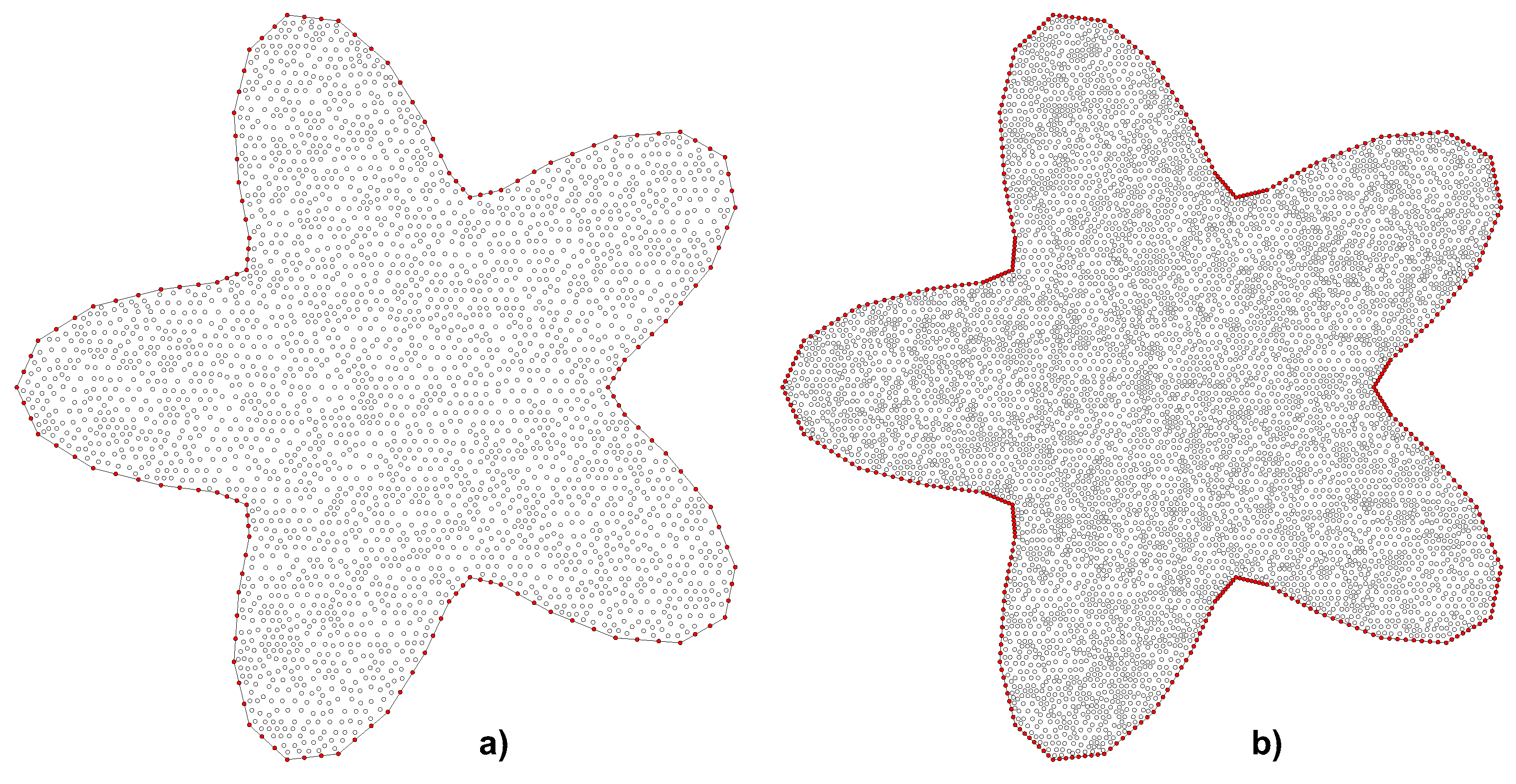
4.2. Example No. 2, Steady Case with Decay

The second example tests steady advection along with tracer decay. For the test, we used an irregular area with two different networks of points—the sparser one has 3216 nodes and the denser one has 6530 points (Figure 6). The coordinates of the boundary points have been computed according to the following formula [8,24]

$$\begin{array}{c}\hfill r\left(\theta \right)=(37-12cos(5\theta \left)\right)/25,0\le \theta \le 2\pi \\ \hfill \{x,y\}=\{rcos(\theta ),rsin(\theta \left)\right\}.\end{array}$$

(35)

Figure 6. Example No. 2—irregular meshes: (a) 3216 points, (b) 6530 points.

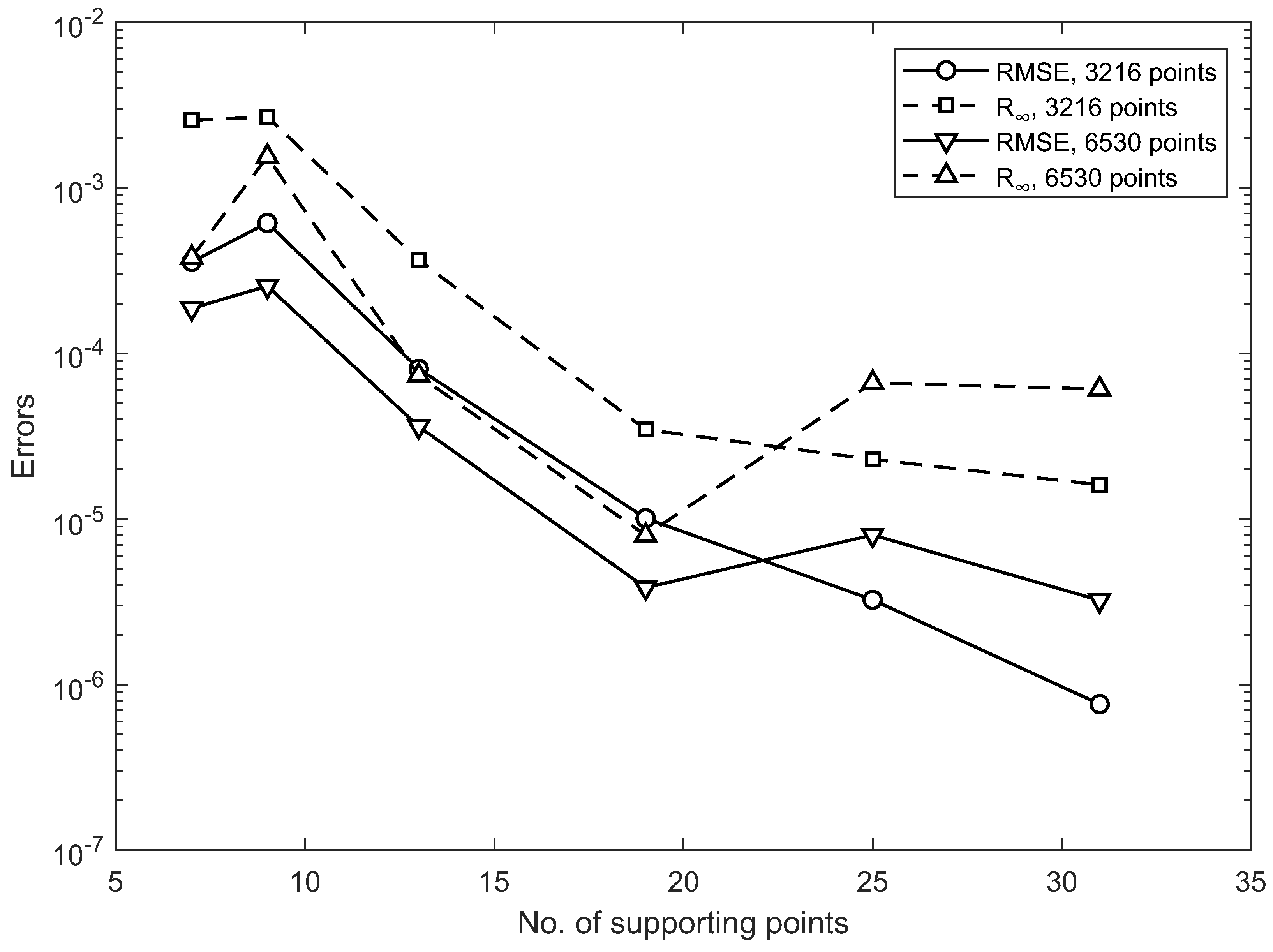
The internal points in both networks have been generated using the Poisson disc algorithm [25,26].

The dispersion and decay coefficients are $D=5$ and $\lambda =4$, respectively. The vector of velocity is constant, $\mathbf{v}=\left(v_x,v_y\right)=(1,1)$. Dirichlet boundary conditions are prescribed at the boundary $\mathsf{\Gamma }$ as

$$C_0\left(\mathbf{x}\right)=e^x+e^y\mathbf{x}\in \mathsf{\Gamma }.$$

(36)

The exact solution is

$$C\left(\mathbf{x}\right)=e^x+e^y\mathbf{x}\in \mathsf{\Omega }.$$

(37)

Similar to the first example, we present a comparison of the accuracy of our modified method for different numbers of virtual points n. We can see from Table 5 that this influence of the number of virtual points on accuracy is negligible.

Table 5. Example No. 2—comparison of RMSE and $R_{\infty }$ for a different number of virtual points.

n	3216 Points		6530 Points
	RMSE	${\mathit{R}}_{\mathit{\infty }}$	RMSE	${\mathit{R}}_{\mathit{\infty }}$
6	1.0489$\times {10}^{-4}$	1.8703$\times {10}^{-3}$	3.3324$\times {10}^{-5}$	6.8178$\times {10}^{-5}$
8	8.0688$\times {10}^{-5}$	3.6588$\times {10}^{-4}$	3.6236$\times {10}^{-5}$	7.3594$\times {10}^{-5}$
10	8.5035$\times {10}^{-5}$	8.2199$\times {10}^{-4}$	3.4279$\times {10}^{-5}$	7.0187$\times {10}^{-5}$
16	8.2809$\times {10}^{-5}$	7.0545$\times {10}^{-4}$	3.5056$\times {10}^{-5}$	7.1266$\times {10}^{-5}$

Table 6 shows the dependence of the accuracy of the method on the number of points in the support. The situation is now different; the number of supporting points m affects the accuracy significantly. The results for both networks used are different.

Table 6. Example No. 2—comparison of RMSE and $R_{\infty }$ for different numbers of supporting points.

m	3216 Points		6530 Points
	RMSE	${\mathit{R}}_{\mathit{\infty }}$	RMSE	${\mathit{R}}_{\mathit{\infty }}$
7	3.57$\times {10}^{-4}$	2.56$\times {10}^{-3}$	1.87$\times {10}^{-4}$	3.79$\times {10}^{-4}$
9	6.13$\times {10}^{-4}$	2.68$\times {10}^{-3}$	2.55$\times {10}^{-4}$	1.54$\times {10}^{-3}$
13	8.07$\times {10}^{-5}$	3.66$\times {10}^{-4}$	3.62$\times {10}^{-5}$	7.36$\times {10}^{-5}$
19	1.01$\times {10}^{-5}$	3.47$\times {10}^{-5}$	3.85$\times {10}^{-6}$	7.96$\times {10}^{-6}$
25	3.25$\times {10}^{-6}$	2.29$\times {10}^{-5}$	8.01$\times {10}^{-6}$	6.65$\times {10}^{-5}$
31	7.63$\times {10}^{-7}$	1.61$\times {10}^{-5}$	3.23$\times {10}^{-6}$	6.09$\times {10}^{-5}$

The error decreases with the increasing number of supporting points in the first sparser network. In the second denser one, the initial decrease is followed by an increase in the error; thus, we can find the optimal number of points in the support (see also Figure 7 and Table 6). The slight deterioration in accuracy when increasing the number of supporting points is probably since the criterion according to [23] at higher numbers leads to an unsatisfactory selection. In these cases, it would probably be better to return to a simple choice based on the distance from point i.

Figure 7. Example No. 2—course of RMSE and $R_{\infty }$ for different numbers of supporting points.

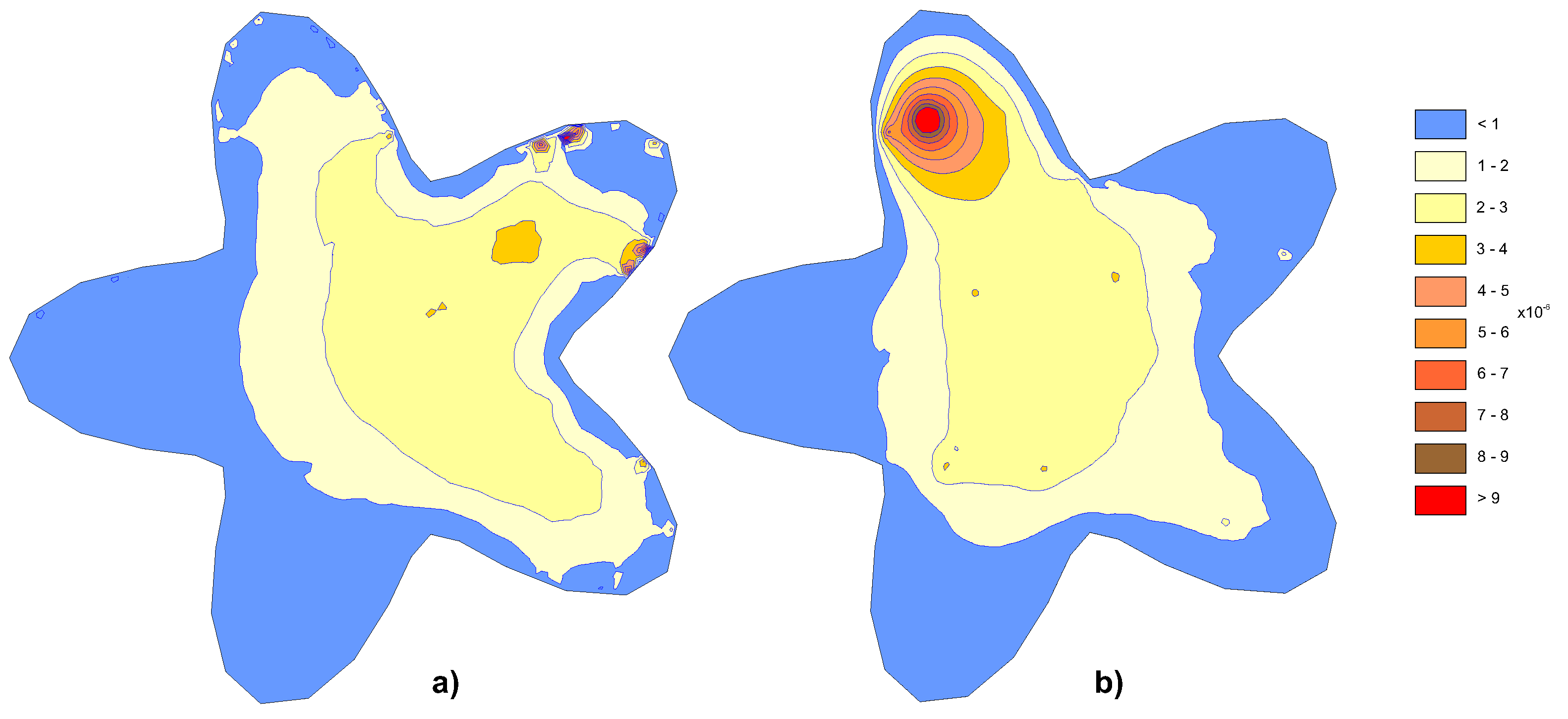
The distribution of absolute errors in the area for both solved networks is presented in Figure 8.

Figure 8. Example No. 2—contours of absolute errors, (a) 3216 points, (b) 6530 points.

As in the previous example, we can also see in Table 7 that it is possible to increase the accuracy of the solution by approximately one order of magnitude by slightly increasing the radius of the virtual area to $r\approx 1.4d_{min}$.

Table 7. Example No. 2—comparison of RMSE and $R_{\infty }$ for different radii of virtual area.

$\mathit{r}/{\mathit{d}}_{\mathit{min}}$	3216 Points		6530 Points
	RMSE	${\mathit{R}}_{\mathit{\infty }}$	RMSE	${\mathit{R}}_{\mathit{\infty }}$
0.6	1.8708$\times {10}^{-5}$	3.7636$\times {10}^{-5}$	5.4936$\times {10}^{-6}$	1.1633$\times {10}^{-5}$
0.8	1.5363$\times {10}^{-5}$	5.6583$\times {10}^{-5}$	4.9468$\times {10}^{-6}$	1.0110$\times {10}^{-5}$
1.0	1.0094$\times {10}^{-5}$	3.4681$\times {10}^{-5}$	3.8808$\times {10}^{-6}$	8.0037$\times {10}^{-6}$
1.2	4.1740$\times {10}^{-6}$	3.5152$\times {10}^{-5}$	2.6612$\times {10}^{-6}$	5.7076$\times {10}^{-6}$
1.4	2.7209$\times {10}^{-6}$	5.8848$\times {10}^{-5}$	1.2998$\times {10}^{-6}$	4.9287$\times {10}^{-6}$
1.6	5.8256$\times {10}^{-6}$	8.4728$\times {10}^{-5}$	2.0681$\times {10}^{-6}$	2.1252$\times {10}^{-5}$

Further, in this example, we tested the shape factor’s influence on the method’s accuracy. It turns out that the accuracy increases slightly with the increasing value of R (Figure 9).

Figure 9. Example No. 2—RMSE and $R_{\infty }$ as functions of the shape factor R.

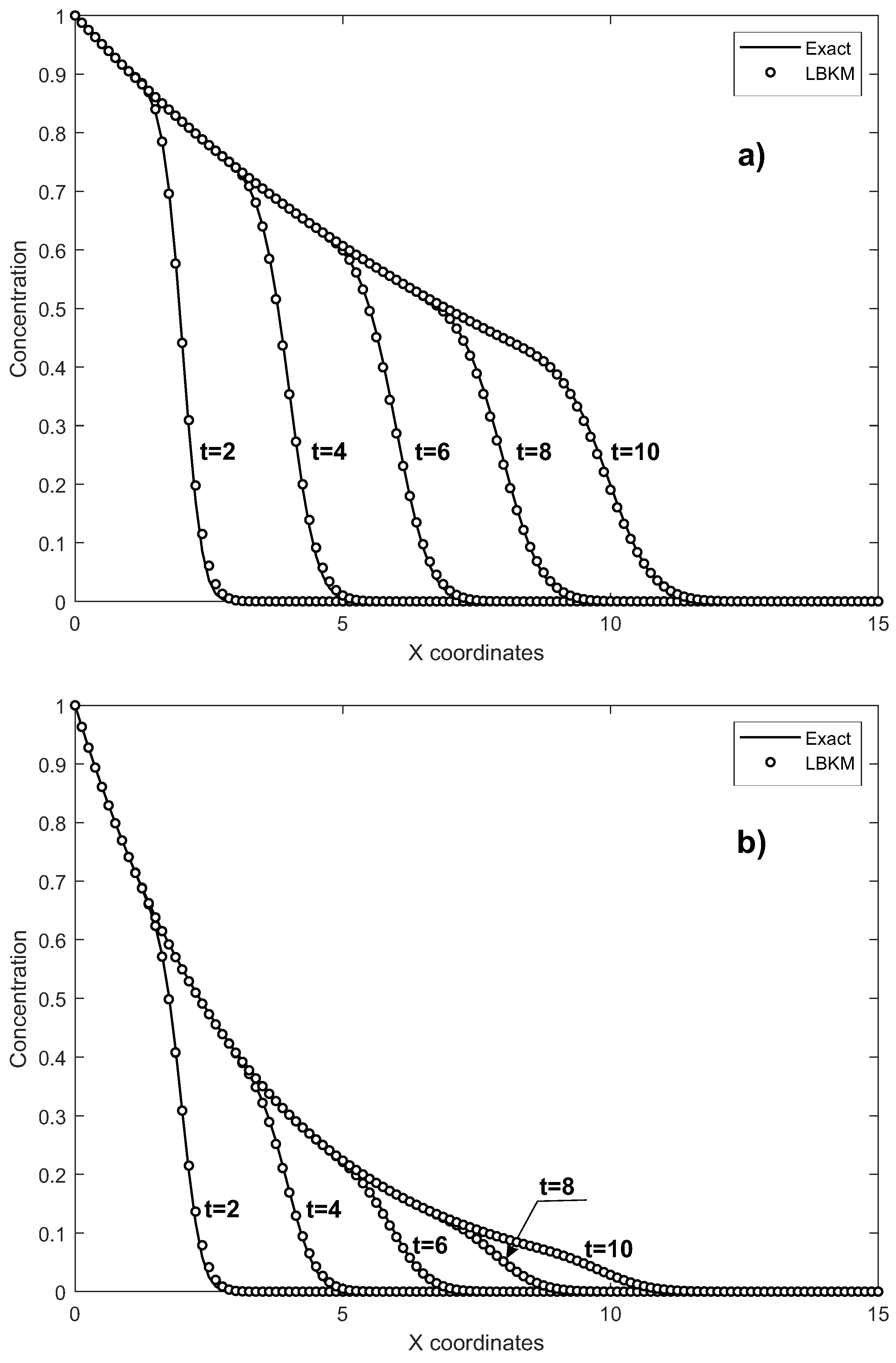
4.3. Example No. 3, Unsteady Case

The third example is the usual case used for testing of the unsteady problem [27,28,29]. The rectangular domain $[0,20]\times [0,2]$ has the initial concentration $C_0=0$ and the Dirichlet boundary conditions $C(0,y)=1$ and $C(20,y)=0$. The Neumann boundary conditions are prescribed as $q(0,x)=q(2,x)=0$. The exact solution is (see e.g., [30])

$$C(x,t)=\frac{C_0}{2}\left[erfc\left(z_1\right)+exp\left(\frac{v_{x}x}{D}\right)erfc\left(z_2\right)\right],$$

(38)

where

$$z_1=\frac{x-v_{x}t}{\sqrt{4Dt}}{z}_2=\frac{x+v_{x}t}{\sqrt{4Dt}}.$$

(39)

The horizontal velocity $v_x=1$ and three diffusion coefficients $D=0.1$, $D=0.05$, and $D=0.02$ have been used. Then, the Peclet numbers (31) are Pe = 200, Pe = 400, and Pe = 1000, respectively. The RBFs with shape functions $\phi \left(r\right)$ according to (14) are used in this example. Two regular meshes of $101\times 11$ and $161\times 17$ points have been used. The total simulation time is $t=10$.

Figure 10 presents the concentration for both networks in the profile $y=1$. Figure 11 then represents the course of the absolute error in this profile. All these results are plotted for times t = 2, 4, 6, 8, and 10.

Figure 10. Example No. 3—concentration profiles for Pe = 1000: (a) Grid $101\times 11$, (b) Grid $161\times 17$.

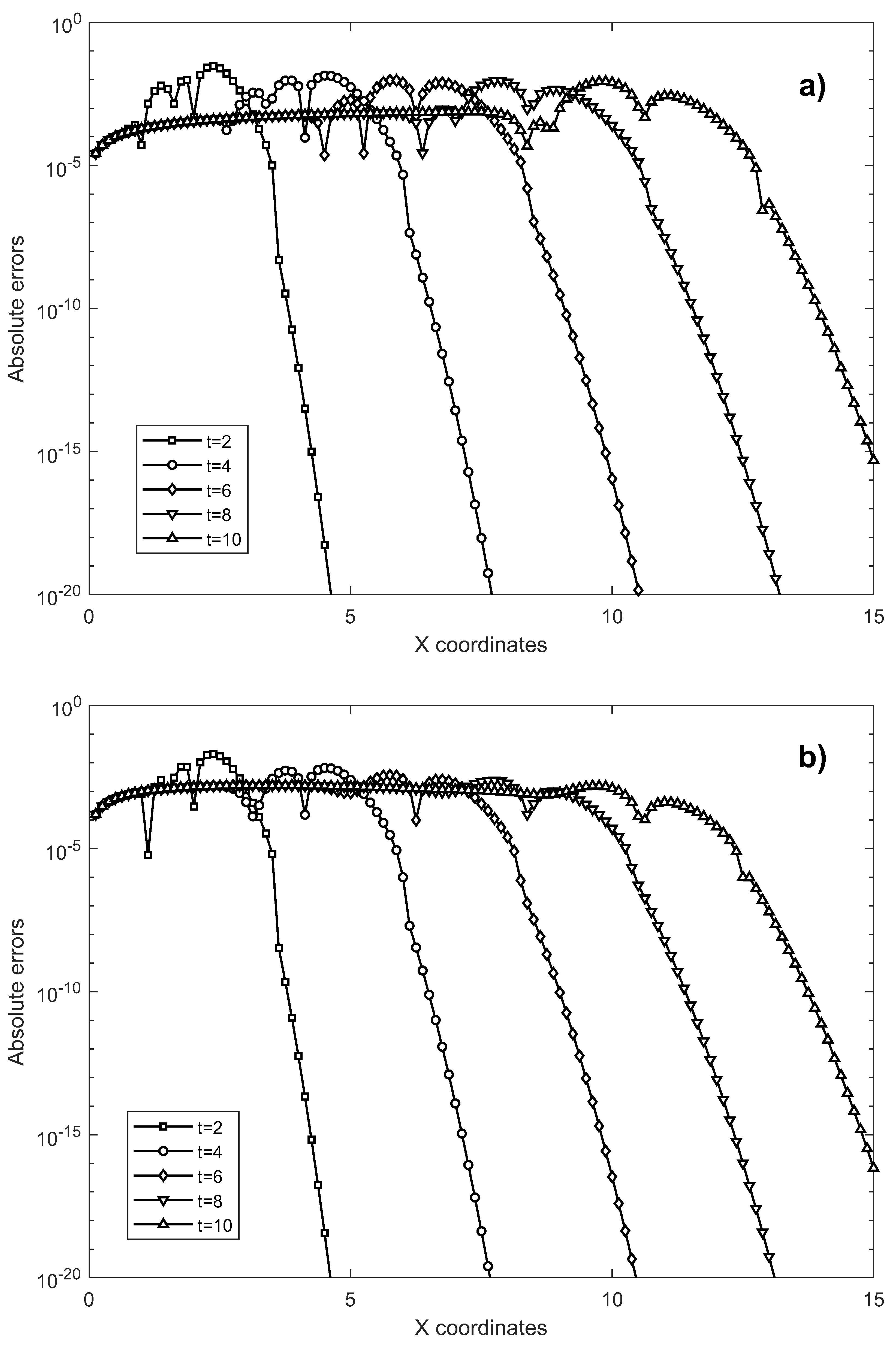
Figure 11. Example No. 3—absolute errors for Pe = 1000, (a) Grid $101\times 11$, (b) Grid $161\times 17$.

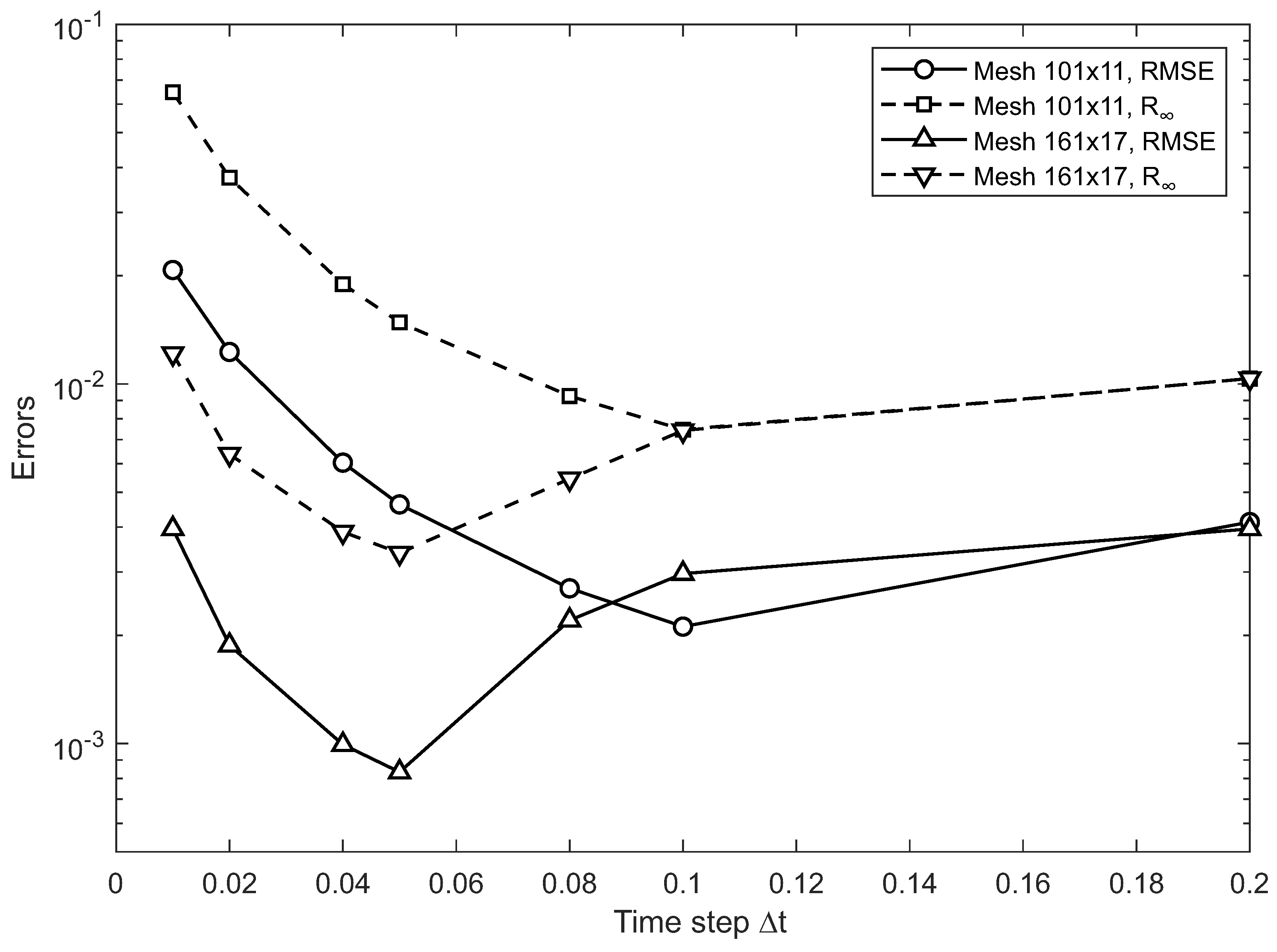
Table 8 clearly shows that the values of RMSE and $R_{\infty }$ decrease when increasing the density of the grid.

Table 8. Example No. 3—RMSE and $R_{\infty }$ for different Peclet numbers.

Pe	Mesh $101\times 11$		Mesh $161\times 17$
	RMSE	${\mathit{R}}_{\mathit{\infty }}$	RMSE	${\mathit{R}}_{\mathit{\infty }}$
200	4.6244$\times {10}^{-3}$	1.4834$\times {10}^{-2}$	8.3319$\times {10}^{-4}$	3.3870$\times {10}^{-3}$
400	1.0440$\times {10}^{-2}$	3.9621$\times {10}^{-2}$	1.2844$\times {10}^{-3}$	5.6586$\times {10}^{-3}$
1000	2.2662$\times {10}^{-2}$	1.0775$\times {10}^{-1}$	4.1826$\times {10}^{-3}$	2.1395$\times {10}^{-2}$

In this example, because it is an unsteady problem, we focused primarily on testing the influence of the time step size and the values of the two shape factors R and $R_P$ on the accuracy of the solution.

Figure 12 shows a comparison of the RMSE and $R_{\infty }$ errors using the various sizes of time steps and Pe = 200. It is clear from Figure 12 that there is an optimal time step for every mesh. Its further refinement only reduces the accuracy of the solution and increases the CPU time.

Figure 12. Example No. 3—RMSE and $R_{\infty }$ as functions of the time step $\mathsf{\Delta }$t.

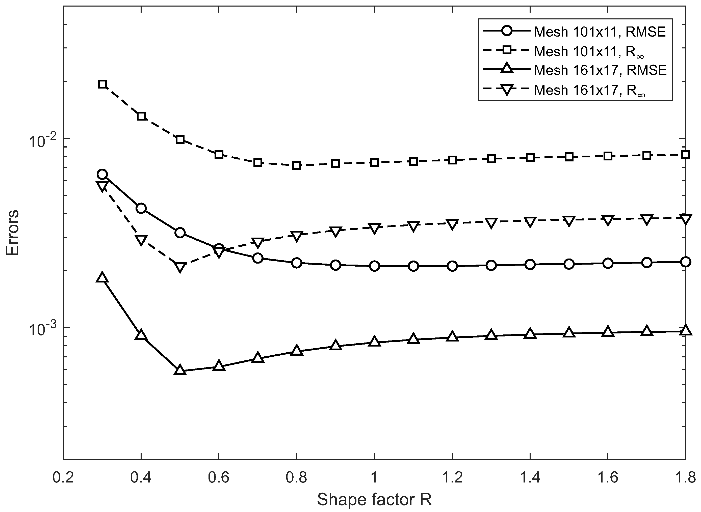
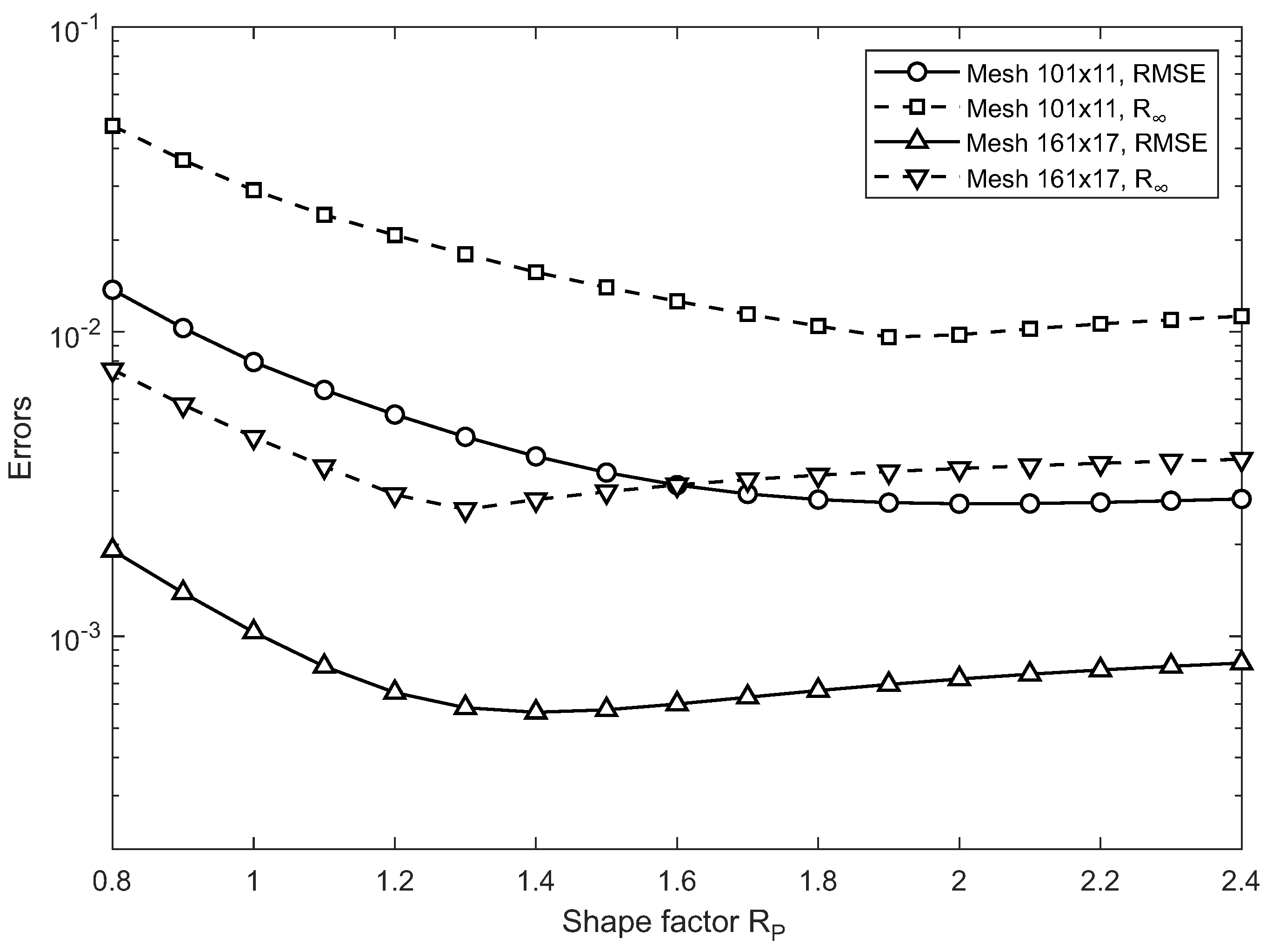
Similar to the previous examples, we monitored the dependence of the accuracy of the solution on the shape factor R of the RBF interpolation for the third example. We also tested the influence of the $R_P$ factor, which is used for the particular solution approximation. These dependencies are plotted in Figure 13 and Figure 14. It can be seen that initially, the error of the method decreases to an insignificant minimum and then the values of RMSE and $R_{\infty }$ stabilize.

Figure 13. Example No. 3—RMSE and $R_{\infty }$ as functions of the shape factor R.

Figure 14. Example No. 3—RMSE and $R_{\infty }$ as functions of the shape factor $R_P$.

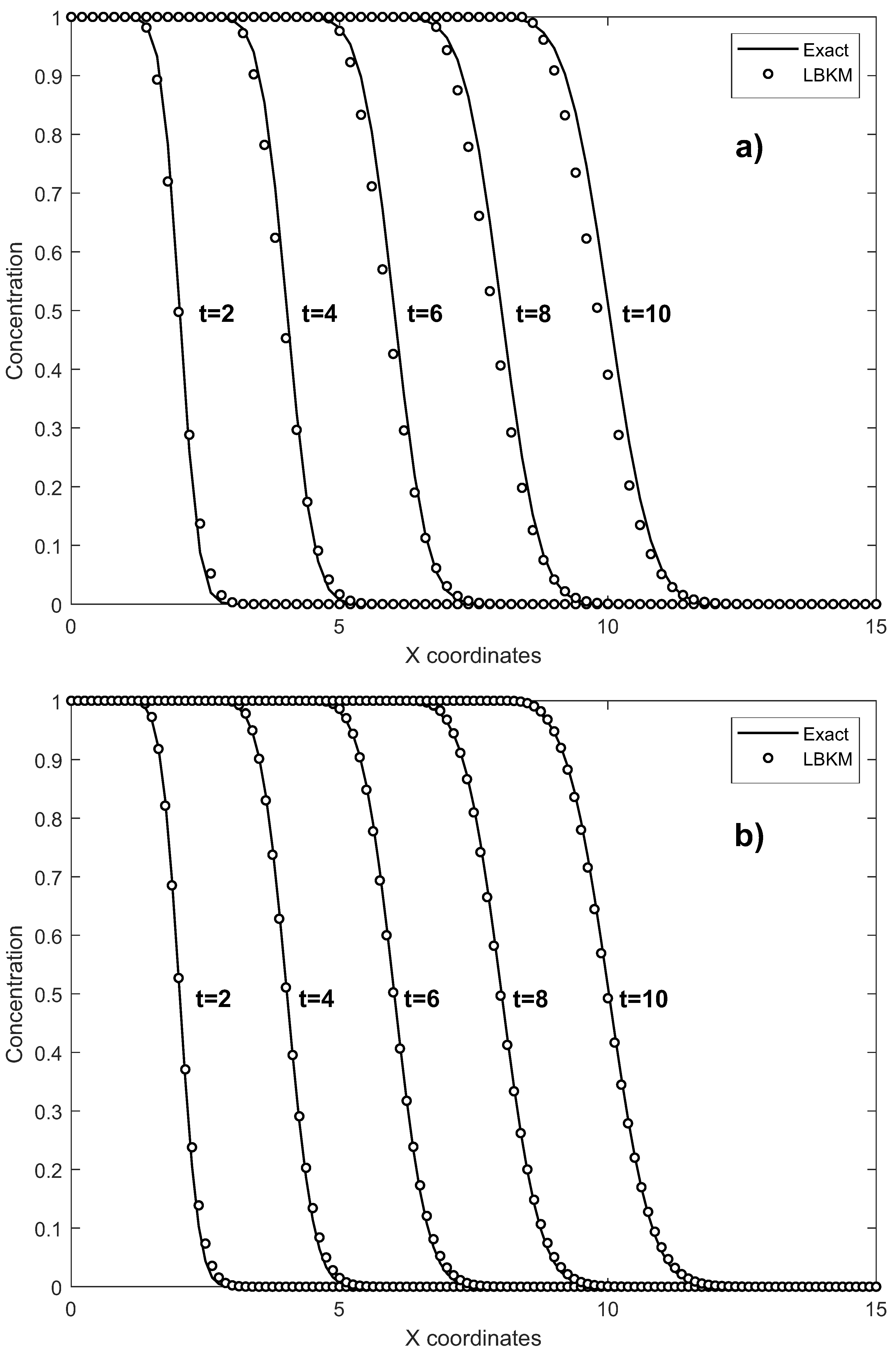
The same rectangular domain with the same two different point meshes as well as boundary conditions is used to test the effect of tracer decay; the decay coefficient values $\lambda =0.1$ and $\lambda =0.3$ are entered. The exact solution is then given as [30]

$$C(x,t)=\frac{C_0}{2}exp\left(\frac{v_{x}x}{2D}\right)\left[exp(-x\beta )erfc\left(z_1\right)+exp\left(x\beta \right)erfc\left(z_2\right)\right],$$

(40)

where

$$\beta =\sqrt{\frac{v_x^2}{4D^2}+\frac{\lambda }{D}}$$

(41)

and $z_1$ and $z_2$ are now

$$z_1=\frac{x-t\sqrt{v_x^2+4\lambda D}}{\sqrt{4Dt}}{z}_2=\frac{x+t\sqrt{v_x^2+4\lambda D}}{\sqrt{4Dt}}.$$

(42)

The course of exact concentration and LBKM results in the profile $y=2$ at time t = 2, 4, 6, 8, and 10 can be seen in Figure 15 for the two different values of the decay coefficient. Figure 16 then shows the course of the absolute errors at the same time intervals.

Figure 15. Example No. 3—concentration profiles for Pe = 1000, mesh 161 × 33: (a) $\lambda =0.1$, (b) $\lambda =0.1$.

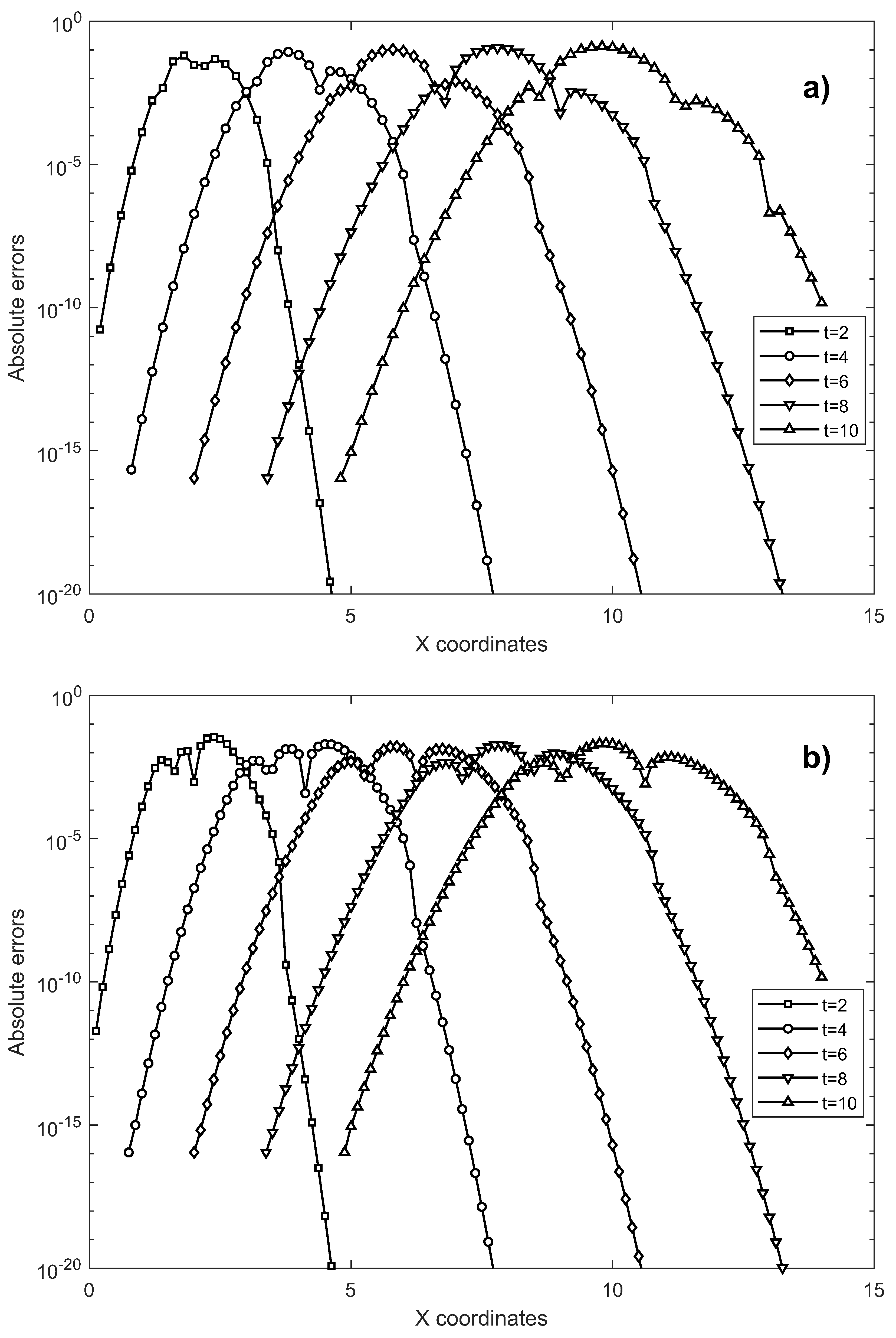
Figure 16. Example No. 3—absolute errors for Pe = 1000, mesh 161 × 33: (a) $\lambda =0.1$, (b) $\lambda =0.5$.

Table 9 shows the RMSE values for $\lambda$ = 0.1 and 0.3 for both used point networks.

Table 9. Example No. 3—comparison of RMSE for Pe = 1000, $\lambda =0.1$, $\lambda =0.3$, and different meshes.

Time	$\mathit{\lambda }=0.1$		$\mathit{\lambda }=0.3$
	Mesh $101\times 11$	Mesh $161\times 17$	Mesh $101\times 11$	Mesh $161\times 17$
2	8.0725$\times {10}^{-3}$	4.0627$\times {10}^{-3}$	5.9374$\times {10}^{-3}$	2.7769$\times {10}^{-3}$
4	8.0044$\times {10}^{-3}$	2.3824$\times {10}^{-3}$	4.5891$\times {10}^{-3}$	1.2482$\times {10}^{-3}$
6	8.8779$\times {10}^{-3}$	1.8665$\times {10}^{-3}$	4.0667$\times {10}^{-3}$	9.8041$\times {10}^{-4}$
8	9.2876$\times {10}^{-3}$	1.7438$\times {10}^{-3}$	3.6041$\times {10}^{-3}$	9.4922$\times {10}^{-4}$
10	9.2755$\times {10}^{-3}$	1.7132$\times {10}^{-3}$	3.2915$\times {10}^{-3}$	9.4261$\times {10}^{-4}$

5. Discussion and Conclusions

In the article, we presented a modification of the local knots method applied to the solution of the advection–diffusion equation. Unlike the previous localizations of the node method, this method uses a regular circular virtual region with evenly spaced virtual points. The boundary knots method is applied to this area. In the next step, this area is connected to the support of the resolved node. Although this procedure is a bit more complicated than the previous methods, it has some significant advantages.

5.1. Condition Numbers

Probably the most significant advantage concerns the reduction of the order of the boundary knots matrix and, thus, also the decrease of the condition number of this matrix. It is possible owing to the fact that the virtual points number is small. It also remains constant for all nodes. Therefore, it was possible to work with this matrix in the presented method using only simple algorithms for solving linear equations or matrix inversion. In addition, it is possible (especially for regular networks of nodes) to design this virtual region equal for all nodes and, thus, to calculate the inverse matrix of the method only once.

In our method, we can distinguish three different condition numbers (CN): local, global, and RBF. The local CN is the condition number of the local matrix A (16). The global CN is the condition number of the global system of equations and is significantly lower than the local one. The RBF condition number refers to the interpolation matrix of radial basic functions (see Table 10). Table 11 contains condition numbers of unsteady case (Example No. 3).

Table 10. Example No. 1—values of condition numbers, eight virtual boundary points.

Pe	Local	Global	RBF
10	4.9691$\times {10}^7$	5.0797$\times {10}^2$	7.5114$\times {10}^5$
30	2.6072$\times {10}^5$	3.0437$\times {10}^2$	7.5114$\times {10}^5$
50	4.6362$\times {10}^5$	2.4988$\times {10}^2$	7.5114$\times {10}^5$

Table 11. Example No. 3—values of condition numbers, eight virtual boundary and six internal points.

Mesh	Local	Global	RBF
101 × 11	6.9144$\times {10}^5$	1.4806$\times {10}^3$	1.8830$\times {10}^7$
167 × 16	7.9764$\times {10}^6$	3.8825$\times {10}^3$	2.8587$\times {10}^7$

The local CN depends substantially on the number of virtual boundary points (see Figure 17). As the number of these points does not influence the precision of our method, we recommend using a maximum of 8 points.

Figure 17. Example No. 1—connection of the local condition number and number of virtual points.

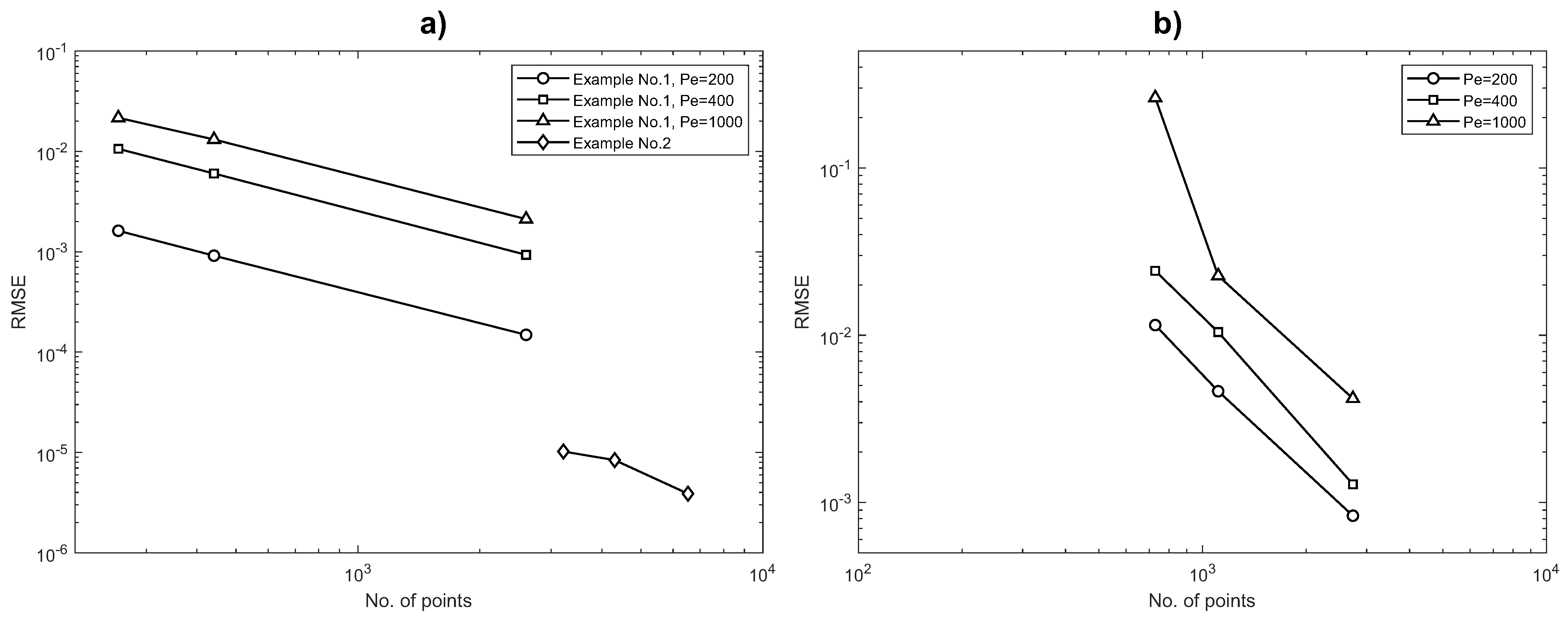
5.2. Convergence Rate

For all three examples, we performed tests of the speed of convergence of the method. For the purposes of these tests, we have additionally added one more sparse network for each example. For the first example, the grid had 16 × 16 points; in the second example, it was an irregular grid with 4305 points; and in the third example, we used a grid of 81 × 9 points. Figure 18 shows the dependency of RMSE on the number of points. To demonstrate the convergence rate (CR) of the present method, the following formula is introduced

$$CR=-\frac{log\left(RMS{E}_1\right)-log\left(RMS{E}_2\right)}{log\left(N_1\right)-log\left(N_2\right)}.$$

(43)

Figure 18. Connection of the RMSE and number of points: (a) steady solution, (b) unsteady solution.

Table 12 contains values of RMSE and convergence rates for examples of the steady case and Table 13 for those of the unsteady transport.

Table 12. Example Nos. 1 and 2—values of RMSE and the convergence rates (CR).

No. of Points	RMSE, Example No. 1			No. of Points	RMSE, Example No. 2
	Pe = 10	Pe = 30	Pe = 50
256	1.619$\times {10}^{-3}$	1.060$\times {10}^{-2}$	2.162$\times {10}^{-2}$	3216	1.023$\times {10}^{-5}$
441	9.140$\times {10}^{-4}$	6.022$\times {10}^{-3}$	1.315$\times {10}^{-2}$	4305	8.390$\times {10}^{-6}$
2601	1.486$\times {10}^{-4}$	9.317$\times {10}^{-4}$	2.114$\times {10}^{-3}$	6530	3.881$\times {10}^{-6}$
CR	1.024	1.052	1.030	CR	1.368

Table 13. Example No. 3—values of RMSE and the convergence rates (CR).

No. of Points	Pe = 20	Pe = 400	Pe = 1000
729	1.150$\times {10}^{-2}$	2.425$\times {10}^{-2}$	2.630$\times {10}^{-1}$
1111	4.624$\times {10}^{-3}$	1.044$\times {10}^{-2}$	2.266$\times {10}^{-2}$
2737	8.332$\times {10}^{-4}$	1.284$\times {10}^{-3}$	4.183$\times {10}^{-3}$
CR	1.984	2.221	3.130

From the values in Table 12, we can conclude that with a regular network of points, the order of the method is slightly above the value of one, and with an irregular network, it is about 30% higher, which may be caused by the different geometric configuration of the irregular networks. In the unsteady state, we see that Houbolt’s method confirms its effectiveness in this case as well, and the values of the rate of convergence are above two.

In the further development of the method, a logical step will be to extend it to 3D tasks or non-linear problems.

References

- Brebbia, C.A.; Telles, J.C.F.; Wrobel, L.C. Boundary Element Techniques; Springer: Berlin, Germany; New York, NY, USA, 1984. [Google Scholar]
- Partridge, P.W.; Brebbia, C.A.; Wrobel, L.C. The Dual Reciprocity Boundary Element Method; CM Publications: Southampton, UK, 1992. [Google Scholar]
- Golberg, M. The method of fundamental solutions for Poisson’s equations. Eng. Anal. Bound. Elem. 1995, 16, 205–213. [Google Scholar] [CrossRef]
- Golberg, M.A.; Chen, C.S. The method of fundamental solutions for potential, Helmholtz and diffusion problems. In Boundary Integral Methods-Numerical and Mathematical Aspects; Golberg, M.A., Ed.; CM Publications: Southampton, UK, 1998; pp. 103–176. [Google Scholar]
- Chen, C.S.; Karageorghis, A. On choosing the location of the sources in the MFS. Numer. Algorithms 2016, 72, 107–130. [Google Scholar] [CrossRef]
- Chen, W.; Fu, Z.; Wei, X. Potential problems by singular boundary method satisfying moment condition. CMES-Comput. Model. Eng. Sci. 2009, 54, 65–85. [Google Scholar]
- Chen, W.; Gu, Y. Recent Advances on Singular Boundary Method. In Proceedings of the Joint International Workshop for Trefftz Method, Kaohsiung, Taiwan, 15–18 March 2011; Volume 4, pp. 543–558. [Google Scholar]
- Kovářík, K.; Mužík, J.; Bulko, R.; Sitányiová, D. Singular boundary method using dual reciprocity for two-dimensional transient diffusion. Eng. Anal. Bound. Elem. 2017, 83, 256–264. [Google Scholar] [CrossRef]
- Kovářík, K.; Mužík, J.; Masarovičová, S.; Sitányiová, D. Regularized singular boundary method for 3D potential flow. Eng. Anal. Bound. Elem. 2018, 95, 85–92. [Google Scholar] [CrossRef]
- Hon, Y.C.; Chen, W. Boundary knot method for 2D and 3D Helmholtz and convection–diffusion problems under complicated geometry. Int. J. Numer. Method Eng. 2003, 56, 1931–1948. [Google Scholar] [CrossRef]
- Chen, W.; Shen, L.J.; Shen, Z.J.; Yuan, G.W. Boundary knot method for Poisson equations. Eng. Anal. Bound. Elem. 2005, 29, 756–760. [Google Scholar] [CrossRef]
- Mužík, J. Boundary Knot Method for Convection-diffusion Problems. Procedia Eng. 2015, 111, 582–588. [Google Scholar] [CrossRef]
- Wang, F.; Wang, C.; Chen, Z. Local knot method for 2D and 3D convection–diffusion–reaction equations in arbitrary domains. Appl. Math. Lett. 2020, 105, 106308. [Google Scholar] [CrossRef]
- Yue, X.; Wang, F.; Li, P.W.; Fan, C.M. Local non-singular knot method for large-scale computation of acoustic problems in complicated geometries. Comput. Math. Appl. 2021, 84, 128–143. [Google Scholar] [CrossRef]
- Zhu, T.; Zhang, J.D.; Atluri, S. A local boundary integral equation (LBIE) method in computational mechanics, and a meshless discretization approach. Comput. Mech. 1998, 21, 223–235. [Google Scholar] [CrossRef]
- Sellountos, E.J.; Sequeira, A. An advanced meshless LBIE/RBF method for solving two-dimensional incompressible fluid flows. Comput. Mech. 2008, 41, 617–631. [Google Scholar] [CrossRef]
- Young, D.; Gu, M.; Fan, C. The time-marching method of fundamental solutions for wave equations. Eng. Anal. Bound. Elem. 2009, 33, 1411–1425. [Google Scholar] [CrossRef]
- Kovářík, K.; Mužík, J.; Bulko, R.; Sitányiová, D. Local singular boundary method for two-dimensional steady and unsteady potential flow. Eng. Anal. Bound. Elem. 2019, 108, 168–178. [Google Scholar] [CrossRef]
- Golberg, M.; Chen, C.; Bowman, H. Some recent results and proposals for the use of radial basis functions in the BEM. Eng. Anal. Bound. Elem. 1999, 23, 285–296. [Google Scholar] [CrossRef]
- Kovářík, K.; Mužík, J.; Mahmood, M.S. A meshless solution of two dimensional unsteady flow. Eng. Anal. Bound. Elem. 2012, 36, 738–743. [Google Scholar] [CrossRef]
- Stevens, D.; Power, H.; Meng, C.Y.; Howard, D.; Cliffe, K.A. An alternative local collocation strategy for high-convergence meshless PDE solutions, using radial basis functions. J. Comput. Phys. 2013, 294, 52–75. [Google Scholar] [CrossRef]
- Reddy, J.; Martinez, M. A dual mesh finite domain method for steady-state convection–diffusion problems. Comput. Fluids 2021, 214, 104760. [Google Scholar] [CrossRef]
- Kovářík, K.; Mužík, J. A meshless solution for two dimensional density-driven groundwater flow. Eng. Anal. Bound. Elem. 2013, 37, 187–196. [Google Scholar] [CrossRef]
- Wang, F.; Chen, W. Accurate empirical formulas for the evaluation of origin intensity factor in singular boundary method using time-dependent diffusion fundamental solution. Int. J. Heat Mass Transf. 2016, 103, 360–369. [Google Scholar] [CrossRef]
- Dunbar, D.; Humphreys, G. A spatial data structure for fast Poisson-disk sample generation. ACM Trans. Graph. 2006, 25, 503–508. [Google Scholar] [CrossRef]
- Wei, L.Y. Parallel Poisson Disk Sampling. ACM Trans. Graph. 2008, 27, 1–9. [Google Scholar]
- Singh, K.M.; Tanaka, M. Dual reciprocity boundary element analysis of transient advection-diffusion. Int. J. Numer. Method Heat Fluid Flow 2003, 13, 633–646. [Google Scholar] [CrossRef]
- Kovářík, K. Numerical simulation of groundwater flow and pollution transport using the dual reciprocity and RBF method. Communications 2010, 12, 5–10. [Google Scholar] [CrossRef]
- Wang, F.; Chen, W.; Tadeu, A.; Correia, C.G. Singular boundary method for transient convection–diffusion problems with time-dependent fundamental solution. Int. J. Heat Mass Transf. 2017, 114, 1126–1134. [Google Scholar] [CrossRef]
- Bear, J. Dynamics of Fluids in Porous Media; American Elsevier Publishing Co.: New York, NY, USA, 1972. [Google Scholar]
Publisher’s Note: MDPI stays neutral with regard to jurisdictional claims in published maps and institutional affiliations. |
© 2022 by the authors. Licensee MDPI, Basel, Switzerland. This article is an open access article distributed under the terms and conditions of the Creative Commons Attribution (CC BY) license (https://creativecommons.org/licenses/by/4.0/).