Article

Ocular Biometrics with Low-Resolution Images Based on Ocular Super-Resolution CycleGAN

Division of Electronics and Electrical Engineering, Dongguk University, 30 Pildong-ro 1-gil, Jung-gu, Seoul 04620, Korea
*
Author to whom correspondence should be addressed.
Mathematics 2022, 10(20), 3818; https://doi.org/10.3390/math10203818
Submission received: 9 September 2022 / Revised: 6 October 2022 / Accepted: 14 October 2022 / Published: 16 October 2022
(This article belongs to the Special Issue Computer Vision and Pattern Recognition with Applications)

Abstract

:
Iris recognition, which is known to have outstanding performance among conventional biometrics techniques, requires a high-resolution camera and a sufficient amount of lighting to capture images containing various iris patterns. To address these issues, research is actively conducted on ocular recognition to include a periocular region in addition to the iris region, which also requires a high-resolution camera to capture images, indicating limited applications due to costs and size limitation. Accordingly, this study proposes an ocular super-resolution cycle-consistent generative adversarial network (OSRCycleGAN) for ocular super-resolution reconstruction, and additionally proposes a method to improve recognition performance in case that ocular images are acquired at a low-resolution. The results of the experiment conducted using open databases, namely, CASIA-iris-Distance and Lamp v4, and IIT Delhi iris database, showed that the equal error rate of recognition of the proposed method was 3.02%, 4.06% and 2.13% for each database, respectively, which outperformed state-of-the-art methods.

1. Introduction

Background of Biometrics

Among various biometrics technologies [1,2], iris recognition is commonly applied in the fields that require personal identification or security above a certain level due to unique characteristics of an iris region (unaffected by aging, no changes in characteristics due to external factors), thus guaranteeing a high level of security [3,4,5,6,7,8]. Iris images are captured from a certain long distance [9], unlike the close-distance iris recognition system environment in which image quality may be reduced. To overcome these drawbacks, replacing the environment or equipment is generally considered first, but entails a high cost. Therefore, ocular or periocular recognition has been researched using an ocular region containing the iris region or periocular region not containing the iris region [10,11]. However, ocular or periocular recognition method also has a problem of low-resolution or poor-quality images when they are captured from a quite far distance or when a low-performance camera is used, which degrades the recognition performance. Super-resolution reconstruction (SRR) may be applied as an alternative to solve the issue [12,13]. However, conventional SRR techniques have been embodied for the purpose of enhancing visibility in images using traditional image processing techniques [14,15]. Thus, ocular recognition performance improvement in low-resolution images cannot be achieved.
In recent years, deep learning technology was advanced, which enables a convolutional neural network (CNN)-based SRR to be extensively conducted [16,17]. Moreover, other studies on SRR have been conducted for applying a generative adversarial network (GAN) [18] to further enhance the performance of SRR [19]. The purpose SRR in general scenes is to improve visibility and increase resolution for the entire image rather than for details of a specific region. However, improvement in recognition performance is considered as a major purpose in biometric images for iris and ocular recognition than improving visibility through SRR as the details of biometrics of each individual are important.
From this perspective, this study proposes an ocular super-resolution cycle-consistent generative adversarial network (OSRCycleGAN)-based SRR method. Our research has contributions in the following three ways compared to previous works:
-
Different from a conventional CycleGAN, our proposed OSRCycleGAN reduces the number of weight filters by half in generator and discriminator. Consequently, it can decrease system complexity and memory usage while increasing the processing speed.
-
The proposed OSRCycleGAN does not use identity loss compared to conventional CycleGAN loss while using cycle consistent and perceptual losses. When calculating the perceptual loss in particular, it calculates authentic and imposter matching dissimilarities between mini-batch unit images in order to reflect them in cycle consistent and discriminator losses.
-
For a fair performance evaluation by other researchers, the trained OSRCycleGAN model and algorithms are publicly available on request.
The rest of the paper is arranged as follows. Previous studies are analyzed in Section 2, while the explanations of OSRCycleGAN-based SRR and the ocular recognition method introduced in this study are provided in Section 3. Experimental results with analyses are presented in Section 4. Finally, conclusions and future works are offered in Section 5.

2. Related Work

Prior studies on iris and ocular recognition can be roughly categorized into those that considered SRR and those that did not consider SRR. The details are provided in the following sections.

2.1. Iris and Ocular Recognition without SRR

Iris recognition in initial phases targeted images taken from a close distance; iris recognition from a long distance has been researched to improve user convenience and to be applicable in a surveillance environment [20,21]. However, long-distance iris recognition requires a sufficiently strong near-infrared (NIR) lighting in addition to a camera with telescopic lens that can maintain high image quality even from a far distance. The iris region in images captured from a long distance has poorer quality than in images captured from a close distance and, therefore, high performance cannot be guaranteed. Accordingly, studies have been conducted using an ocular region including the iris, which is larger than the iris region.
An ocular region can be captured from a farther distance than the convention iris recognition method. Therefore, it can be obtained relatively easily although rich and unique features of iris cannot be used, and the rough iris region has been used as a substitute in the conventional iris recognition [22,23] and integrated in iris recognition methods [10,24,25]. Oishi et al. [24] proposed a method involving fusion of two scores of iris recognition and periocular recognition. Tan et al. [25] also obtained iris recognition result and periocular region recognition result through fusion.
The above methods are handcrafted feature-based methods, and deep feature-based methods have been recently researched to improve recognition performance. In a study by Gangwar et al. [26], after extracting a circular iris region from the input image as in conventional iris recognition methods, the region was then converted to a rectangular iris region in a polar coordinate for an input in the CNN for recognition. In a study by Lee et al. [27], when an iris image quality is poor in a noisy environment, a total of three images are captured by expanding the iris region with respect to the center of pupil and then the images are input in three CNN models for recognition. Liu et al. [28] applied the Hough transform as a preprocessing step of an input to detect the iris boundary to improve the iris recognition performance; then, an input image was configured by making the region excluding the iris region fuzzy using the Gaussian low-pass filter, and a CNN model was trained using the image to perform recognition. Vizomi et al. [29] attempted ocular recognition by applying a CNN. Lee et al. [30] obtained the ocular region using a rough pupil detection method from the face image captured by an NIR sensor and trained a deep CNN using this region.
However, all these studies focused on iris and ocular recognition without considering SRR, which implies degradation in recognition performance when low-resolution images are input.

2.2. Iris and Ocular Recognition with SRR

2.2.1. Conventional Image Processing-Based Method

There are studies that have applied SRR for restoring low-resolution images in a recognition system using iris and ocular regions. Nguyen et al. [21] detected the iris region in each image of a video sequence captured from a long distance and then determined whether each detected iris region has high resolution and high quality. Subsequently, Nguyen et al. [31] modeled the relationship between the original high-resolution iris image and the low-resolution iris image, which was then converted to feature-domain based on a maximum a posteriori probability (MAP) for SRR. Deshpande et al. [32] used Papoulis–Gerchberg (PG) and projection onto convex set (POCS) methods as SRR for improving the quality of a low-resolution iris image. In a study by Nguyen et al. [33], focus score weighted SRR was applied to restore low-resolution and low-quality images for performing iris recognition in images captured from a long distance and in a moving uncooperative environment.

2.2.2. Learning-Based Method

Traditional image processing-based SRR methods have limitations in performance improvement as the degradation function, which is the cause of degradation in quality of captured images, needs to be presumed by humans and the image restoration process is fairly difficult to perform. Thus, learning-based SRR methods have been researched. In a study by Fahmy et al. [34], a cross-correlation model was used to register and align the divided image into nine frame sets to apply SRR. Shirke et al. [35] applied the SRR method developed by Fahmy et al. [34] to restore iris images acquired from a distance for improving resolution and performance. In a study by Cui et al. [36], iris images were synthesized without a large iris image dataset due to the difficulty in constructing an iris image dataset during which PCA-based SRR was applied to improve the resolution and quality of images. Shin et al. [37,38] proposed a recognition method in which a low-resolution iris image is restored using multi-layered perceptron (MLP). Moreover, Shin et al. [39] proposed a method for generating and recognizing a high-resolution iris image using MLP and constraint least square (CLS) filter. Alonso-Fernandez et al. [40] proposed a PCA hallucination method in which low-resolution (LR) patches are obtained using PCA eigen-transformation from a low-resolution input image and then high-resolution (HR) patches for the training dataset are obtained to restore a high-resolution iris image.

2.2.3. Deep Feature-Based Method

Traditional learning-based methods have the disadvantage of limited improvement in SRR performance for images captured in various environments; therefore, deep learning-based methods have been researched. In a previous study [41], an iris super-resolution method involving a CNN model consisting of three general layers that restore LR patch to HR patch, and a stacked auto-encoder containing several auto-encoders was proposed. In a study by Reddy et al. [42], an ocular sequence image was captured, and subpixel registration was first performed using a discrete cosine transform interpolation filter (DCTIF) for images in each frame. Ocular recognition was then performed by applying deblurring using an additional CNN for the ocular sequence image. In another study [43], texture or natural image was pre-trained with a CNN model and the weight was trained as well; then, transfer learning for learning iris images was applied to an SRCNN model and very deep convolutional networks (VDCNN) model.
In advanced deep learning-based methods, they conducted various experiments such as image steganography using GAN and attention modules [44,45,46]. In [44], they performed image steganography by using called CHAT-GAN implemented by GANs combined with a channel attention module. Based on this method, they achieved high-performance for image steganography without losing hiding information and image qualities. In a study by Liao [45,46], they proposed a new method that decreases or distributes the payload in color image steganography. Image steganography is quite difficult to implement because its goal is to hide additional key information in an image without any noticeable differences. In other words, the method may have high system complexities if implemented. Therefore, they attempted to decrease or distribute the payload by proposing a method based on image texture complexity and distortion distribution. As a result, they got a satisfactory performance by implementing the proposed method called embedding strategy based on image texture complexity (ES-ITC), embedding strategy based on distortion distribution (ES-DD), and amplifying channel modification probabilities strategy (ACMP).
In the wild, various degradation factors can reduce image quality, and these factors may appear at any time, which cannot be noticed. This can decrease system performance, so these factors should be removed. Based on this background, Yin et al. [47] proposed a method that eliminates the degradation factor and obtains the super-resolution image by single conditional hyper-network architecture.
The deep learning-based methods explained above all use general CNNs or encoders, thus having limitations in SRR and performance improvements for iris and ocular images in various environments, which is caused by not using the scheme of competitive training of generator and discriminator. This study, therefore, proposes an OSRCycleGAN based SRR method for improving the SRR performance through competitive learning of generator and discriminator, and a method for improving recognition performance of ocular images captured at a low resolution.
Table 1 below compares the strengths and weaknesses between previous studies and the proposed method.

3. Proposed Method

3.1. Overview of Proposed Method

Figure 1 shows the overview of the proposed method. A low-resolution ocular image is used as an input (Step 1 of Figure 1). This is converted to a high-resolution ocular image by OSRCycleGAN proposed in this study (Step 2 of Figure 1). Then, the restored image is used as an input of a residual neural network (ResNet) pretrained with ocular images; ocular features are extracted from a pooling layer before the last fully connected layer (FCL) (Step 3 of Figure 1). Matching distance is calculated based on the Euclidean distance between the features extracted from the input image and the features extracted from the registered image. It is accepted as genuine matching if the calculated distance is less than the threshold and rejected as imposter matching otherwise (Step 4 of Figure 1).

3.2. SRR by OSRCycleGAN

In general, the process of capturing a low-resolution image can be represented in the equation [48,49].
y = H ( x ) + n
Here, y ,   x ,   H ( · ) , and n refer to low-resolution image, original high-resolution image, degradation function, and additional noise, respectively. In this equation, H ( · ) is the two-dimensional point spread function (PSF) that degrades the quality of the original image x. Accordingly, accurately modeling PSF and n improves SRR performance, but it is still difficult to accurately model low-resolution images captured in various environments. Accordingly, this study proposes an OSRCycleGAN-based SRR method.

3.2.1. Architecture of CycleGAN

OSRCycleGAN proposed in this study is based on a cycle-consistent generative adversarial network (CycleGAN) model. In the SRR method involving only a general CNN or an encoder, the original form of the image being restored is not maintained well or the image information is not considered during restoration. The model is trained in one direction for the region viewed by the filter based on the calculation of the weight of simple convolution filtering. Conversely, CycleGAN [50] has been mostly applied in image translation and style transfer. Style is learned by learning the difference between each domain through cycle loss and image generating capability of a GAN based on which loss is reflected in the GAN so that an image of another domain can be generated in one desired domain. In this study, CycleGAN is used for high-resolution image reconstruction rather than for style transfer or image translation. If each domain is, respectively, designated as low resolution and high resolution, the result of our image SRR can be attained when an image is transformed from the low-resolution to the high-resolution fields to be produced via GAN and cycle loss.
CycleGAN generally consists of two generators and two discriminators in which a generator generates images having the difference between domains and a discriminator discerns the difference between the image generated by converting the domain and the ground-truth image of the respective domain. Equation (2) below shows how generators G ( · ) and F ( · ) that had received x ,   y as input and ground truth are processed in CycleGAN. Here, x is the low-resolution image, while y is the respective high-resolution image input.
x = F ( G ( x ) ) ,       y = G ( F ( y ) )
G ( · ) : X Y ,                   F ( · ) : Y X
Here, G ( · ) and F ( · ) each represent generators which generate images for the domain characteristics of X > Y and Y > X , respectively. Using two generators is the unique characteristic of CycleGAN where the generator that converts X > Y gives the input x to G ( · ) to obtain y ˜ and then goes through F ( · ) to obtain x . Similarly, the same process is followed for the opposite case of Y > X . The difference is calculated when the model is back to X > Y > X or Y > X > Y through conversion between domains and generation using two generators, and this difference can be reduced to perform conversion between the targeted domains more accurately. The equation for calculating this process is called cycle loss, as expressed in Equation (4) below.
c y c ( G ,   F ) = E x ~ P d a t a ( x ) [ F ( G ( x ) ) x 1 ] + E y ~ P d a t a ( y ) [ G ( F ( y ) ) y 1 ]
Here, x is the low-resolution image, while y is the respective high-resolution image input. Because G ( · ) and F ( · ) each represent generators which generate images for the domain characteristics of X > Y and Y > X , respectively, F ( G ( x ) ) shows x image (as shown in Equation (2)) obtained by X > Y > X while G ( F ( y ) ) represents y image (as shown in Equation (2)) obtained by Y > X > Y . x ~ P d a t a ( x ) and y ~ P d a t a ( y ) are data distributions. · 1 shows L1 distance, and E represents expectation value.
The discriminator is trained so that it cannot distinguish between the image generated by the generator and the ground-truth image, and this process can be referred to as adversarial loss. Equations below show the adversarial loss of X > Y and Y > X .
adv ( G ,   D Y ,   X ,   Y ) = E y ~ P data ( y ) [ log D y ( y ) ] + E x ~ P data ( x ) [ log ( 1 D y ( G ( x ) ) ]
adv ( F ,   D X ,   Y ,   X ) = E x ~ P data ( x ) [ log D x ( x ) ] + E y ~ P data ( y ) [ log ( 1 D x ( G ( y ) ) ]
Here, D y ( y ) represents the discriminator using y (real high-resolution image) as input, and D y ( G ( x ) ) shows the discriminator using G ( x ) (generated (fake) high-resolution image by the generator G ( · ) using x (low-resolution image) as input). In addition, D x ( x ) represents the discriminator using x (real low-resolution image) as input, and D x ( G ( y ) ) shows the discriminator using G ( y ) (generated (fake) low-resolution image by the generator G ( · ) using y (high-resolution image) as input). The log( · ) is a logarithmic function.
Based on Equations (4)–(6), the final CycleGAN loss is as follows.
( G ,   F ,   D X ,   D Y ) = a d v ( F ,   D X ,   Y ,   X ) + a d v ( G ,   D Y ,   X ,   Y ) + c y c ( G ,   F )

3.2.2. Architecture of OSRCycleGAN

The process of converting low-resolution ocular image to a high-resolution image based on OSRCycleGAN is shown in Figure 2, where the image y , which corresponds to the conversion result of generator G x ( · ) , is the final restored high-resolution image. OSRCycleGAN reduces the number of weighted filters by half to reduce the number of parameters in a conventional CycleGAN model; consequently, system complexity and memory usage are reduced, and processing speed is increased by reducing the channel dimension of a feature map. Parallel computation through graphics processing unit (GPU) is essential for applying deep learning in which an increase in the number of weighted filters requires high-performance GPU for training and testing, thus being difficult to be applied in diverse environments.
The generator model of OSRCycleGAN was modified to reduce the channel dimension based on a six-layer model consisting of residual connection with batch normalization (BN). The discriminator model was also modified in the same manner. Table 2 and Table 3 present the details of generator and discriminator of OSRCycleGAN used in this study. The ocular image used in this study includes the information of the eyelid, eyelash, pupil, iris, and sclera. The general shape of the eye is longer width-wise than length-wise. Therefore, a rectangular shape, as shown in Table 2 and Table 3, was used, instead of a square shape, as an input in a conventional CycleGAN to prevent the information from being lost. Because the basic architecture of proposed OSRCycleGAN is referred to the original CycleGAN, we followed the positions of BN batch normalization based on the structure of original CycleGAN.

3.2.3. Loss of OSRCycleGAN

In OSRCycleGAN, identity loss used in CycleGAN loss was eliminated, and the perceptual loss shown in Equation (8) was applied to improve the SRR performance as shown in Figure 2c.
pct = 1 T ( C ( y i ) 1 T C ( y i )   C ( x i ) 1 T C ( x i ) ) 2     for   i = 1 T
Equation (8) expresses a perceptual loss used for our proposed method. First, each ground truth image and restored image by proposed OSRCycleGAN are passed in ResNet-101 model. Here, ResNet-101 model is denoted by C ( · ) . Ground truth image and restored image are denoted by y and x , respectively. In addition, the ith extracted features from average pooling layer of the model C ( · ) are represented as C ( y i ) and C ( x i ) , respectively, and T is 2048. Using Equation (8), the difference of mean is calculated for each 2048 feature, and they are summated. From that, the dissimilarity between restored and original (ground truth) image is calculated as shown in Equation (8).
Rather than simply calculating the loss by comparing the restored image with the ground-truth image, features were extracted by having the images restored at a mini-batch unit input in the previously trained CNN model, and the distance between the extracted feature and the feature of ground-truth image was calculated based on authentic and imposter matching to be reflected in the GAN loss. When this loss is used, a significant effect can be observed on the final GAN loss depending on the distance value. The loss value increases as the distance increases so that inadequate restoration can be reflected in the model through which better restoration results can be expected. For extracting features to calculate the perceptual loss, a ResNet model pretrained with ocular images was used. Ultimately, cycle consistent loss of Equation (7) and perceptual loss of Equation (8) were used together in OSRCycleGAN, as expressed in Equation (9).
loss = ( G ,   F ,   D x ,   D y ) + pct

3.2.4. Difference between OSRCycleGAN and Original CycleGAN

In this section, the differences between the proposed OSRCycleGAN and the original CycleGAN are presented:
-
Different from a conventional CycleGAN, our proposed OSRCycleGAN reduces the number of weight filters by half in generator and discriminator. Consequently, it can decrease system complexity and memory usage while increasing the processing speed.
-
The proposed OSRCycleGAN does not use identity loss compared to conventional CycleGAN loss while using cycle consistent and perceptual losses. When calculating the perceptual loss in particular, it calculates authentic and imposter matching dissimilarities between mini-batch unit images in order to reflect them in cycle consistent and discriminator losses.

3.3. Ocular Recognition

In this study, ResNet-101 was used for ocular recognition based on the results of a previous study [30]. Generally, when only the layer depth is extended without any supplementation, training accuracy is reduced, and global minimum cannot be reached because repeatedly processing convolutions causes features of the original image to be reduced through computation and, thus, loses characteristics. This problem was solved by using the concept of identify mapping and short-cut-(skip-connection)-based residual block. For training with the datasets used in this study, fine-tuning was proceeded based on a pre-trained ResNet model [51]. Several hundreds of thousands of datasets are required to train the weights of many layers in ResNet, and the experimental dataset used in this study is insufficient. This model was pre-trained with ImageNet database, which consists of several hundreds of thousands of images [52] and was used in ImageNet large-scale visual recognition competition (ILSVRC). Therefore, the image size is resized into the input size of the ImageNet data in this study. Here, it is determined in which layer fine-tuning is performed for retraining. In this study, only Conv5 and the fully connected layer were fine-tuned. Several hyper-parameters and optimizers need to be selected for training a CNN. Most processes of model training can be separated into forward and backward ones. The forward process arbitrarily initializes the weight, and the computation is proceeded sequentially according to how the model is designed. Then, in the backward process, the desired ground-truth value and the value computed in the forward process are compared to calculate the loss, which is then used to adjust the weight in backward. An activation function is considered important in the forward process. A sigmoid function was used commonly in the past, but due to an extensive period of time and computation amount, a rectified linear unit (ReLU) [53] is more commonly used an activation function recently. A ReLU function is easy to compute and does not output negative values, thus exhibiting a better performance when training is converged and not requiring extensive computation for finding a slope value.
A basic multinomial logistic loss is used in ResNet for which the jth output ( σ ( z ) j of Equation (10)) predicted using the softmax function in Equation (10) was used for calculation. Accordingly, numerical stability can be maintained when calculating the slope.
σ ( z ) j = e z j k = 1 K e z k     f o r   j = 1 ,   K
Here, K is the number of outputs (classes) of ResNet. In case that the array of output neurons is set to z , the probability of the neurons belonging to the jth class is obtained by dividing the value of the jth class by the sum of the values of all classes. Using the calculated results as input, a multinomial logistic loss (MLL) of Equation (11) [54] is calculated, as expressed in Equation (11).
MLL = 1 K n = 1 K log ( p ^ n , l n ) ,
Here, p ^ n represents predicted probability, and l n is a ground-truth label ( l n     [ 0 ,   1 ,   2 ,   ,   K 1 ]   among   the   K   classes ).
In most studies related to biometrics, measuring a recognition performance is in a closed world and open world settings. Closed world setting is when the classes of data for training and testing are the same, while open world setting is when the classes of data for training and testing are different. Typically, it is difficult to presume that the classes of data for training and testing biometrics are the same. Thus, open world setting is deemed more appropriate for real-world applications and, thus, was adopted in this study as well. In the biometrics classification, the output of an FCL of the CNN is used or the feature vector extracted from the layer before the last FCL is used to calculate the matching distance from the feature vector of the registered image. In closed world setting, the classes of data for training and testing are the same. Therefore, the output of an FCL of CNN can be directly used; in open world setting, as the classes of data for training and testing are different, the feature vector extracted from the layer before the last FCL is used to calculate the matching distance from the feature vector of the registered image to perform recognition.
In this study, ocular images processed by SRR using OSRCycleGAN are inputted to ResNet which extracts the 2048 features from the average pooling layer. A total of 2048 features are used to calculate the Euclidean distance from the 2048 features extracted from the enrolled ocular image. It is accepted as genuine matching if the calculated distance is smaller than the threshold, and rejected as imposter matching otherwise. With the training data, the optimal distance threshold was set at the point where false acceptance error (FAR) is identical to false rejection error (FRR). FAR denotes the error of incorrectly determining imposter data as genuine, whereas FRR incorrectly denies genuine data as an imposter. FAR and FRR generally have a tradeoff relationship, and the error when FAR is identical to FRR is named as the equal error rate (EER).

4. Experimental Results

4.1. Dataset and Experimental Environments

To evaluate the performance of the proposed method, the experiment was conducted using three open databases obtained with an NIR camera: CASIA-Iris-Distance and CASIA-Iris-Lamp [55], and Indian Institute of Technology Delhi (IIT Delhi) databases [56]. Each database was divided into two sub-sets to conduct twofold cross-validation. For example, 282 classes including two eyes of 141 individuals in the CASIA-Iris-Distance database were divided into sub-database 1 (DB 1) of 142 classes (71 individuals) and sub-database 2 (DB 2) of 140 classes (70 individuals) to perform data augmentation before conducting training. For data augmentation, translation and cropping were applied for six pixels in all four directions to augment the data by 169 times [30]. Data augmentation based on translation and cropping has been commonly used to other previous studies [57]. Hence, misalignment between registered and recognition images was covered by training the CNN, and the problem of inadequate training from having insufficient dataset was solved. Furthermore, the augmented data were only used for training, while the original data were used for testing. By separately conducting training and testing through twofold cross-validation, the problem of overfitting, which leads to degradation in performance for testing data, caused by the training data being excessively trained by CNN, was prevented. The average accuracy attained from two testing by twofold cross-validation was utilized as the final accuracy of the proposed method. Table 4 depicts the detailed descriptions of the experimental databases used in the study.
Bilinear interpolation was used with respect to the original ground-truth image in Table 4 to compose low-resolution images having 1/16 resolution of the original images. In actual environments, Gaussian blur was additionally applied to compose a dataset considering how a blur or other types of noises may occur due to movements.
Training and testing of the proposed method were conducted in a desktop computer installed with central processing unit (CPU) Intel i7-6700 3.40 GHz, random access memory (RAM) of 32 GB, and NVIDIA GeForce GTX1070 graphic processing unit (GPU) [58]. Compute unified device architecture (CUDA) of version 8.0 and CUDA deep neural network library (cuDNN) of version 5.0 were employed; our algorithms were made using open computer vision (OpenCV) of version 3.3.0 and Visual Studio 2015. TensorFlow of version 2.1.0 [59] and Windows Caffe of version 1.0.0 [60] were used for the implementation of OSRCycleGAN and ocular recognition model, respectively.

4.2. Training of the Proposed Model

Training of OSRCycleGAN

For the hyper-parameters for training OSRCycleGAN that restores high-resolution images, 200 epochs of repeated training, mini batch size of 10, and Adaptive moment estimation (Adam) as optimizer [61] were applied. Beta_1, which is a parameter for Adam, was 0.5 for which the initial learning rate was 2 × 10 4 for the exponential decay rate of Adam optimizer. For the estimate of first and second moment, 0.9 and 0.999 were applied, respectively. We did not employ learning rate strategies, i.e., linear decay. These values were maintained in all the experiments. When training SRR models using the dataset used in previous studies on SRR and in this experiment, the hyper-parameters of the proposed model were applied under the same condition for a fair evaluation. To solve the inherent problem of a GAN where a generator is difficult to train, the generator was repeatedly trained for five times, while the discriminator was trained once for one mini batch. Due to this training strategy, the optimization of generator of OSRCycleGAN model was possible along with discriminator. Figure 3 depicts the loss graphs of generator and discriminator of OSRCycleGAN. As depicted in Figure 3, OSRCycleGAN was trained enough with the training data.
We adopted twofold cross-validation because the previous deep learning-based ocular recognition study [30] has chosen the same twofold cross-validation. In our research, we do not focus on ocular recognition method but ocular super-resolution reconstruction by OSRCycleGAN. Therefore, we adopted the ocular recognition method of [30] in our research, and we used the same twofold cross-validation in order to follow the experimental protocol of [30]. Additionally, we added the valid loss plots in Figure 3, which were obtained with validation data. We set 10% of training data as validation data, and these validation data were not used for training. As shown in Figure 3, validation loss graphs are also decreased and stabilized according to the increment of epochs, which confirms that our OSRCycleGAN was not overfitted with training data.
Stochastic gradient descent (SGD) optimizer [62] was used for training the ResNet-101, during which a step policy was used as a learning rate policy for optimization where a gamma value is multiplied at a certain iteration. As one of the characteristics of SGD, training was conducted at the mini-batch size unit. Each model in the study was trained for 3–10 epochs. The learning rate was set to 0.0001, which is fairly small as fine-tuning was proceeded using the pre-trained weight. Momentum and weight decay values were set to 0.9 and 0.0001, respectively, while the gamma value was set to 0.1. Each dataset consisted of a different number of images, accordingly, the number of steps was varied in order to achieve the optimal performance. Figure 4 shows the graphs of training accuracy and training loss obtained during training of the ResNet-101 model. As shown in Figure 4, training loss almost went to 0, while training accuracy converged to 100% as the training epoch increased, which indicates that the ResNet-101 model used in this study was successfully trained.

4.3. Testing of the Proposed Method

4.3.1. Ablation Studies

To evaluate the performance of SRR by OSRCycleGAN, the similarity between the original high-resolution image and the image restored by SRR was measured using signal-to-noise ratio (SNR) [63], peak signal-to-noise ratio (PSNR) [64], and structural similarity (SSIM) [65], as expressed in Equations (12)–(15). The SRR performance is higher as all the values of SNR, PSNR, and SSIM are high.
MSE = 1 m n i = 0 m 1 j = 0 n 1 [ I o ( i ,   j ) I e ( i ,   j ) ] 2
SNR = 10 log 10 ( i = 0 m 1 j = 0 n 1 [ I o ( i ,   j ) ] 2 m n MSE )
PSNR = 10 log 10 ( 255 2 MSE )
Here, Io is the original high-resolution image, while Ie is the image obtained with SRR. m and n indicate width and height of the image, respectively. Equation (15) below shows the mathematical equation of SSIM.
SSIM = ( 2 μ e μ o + C 1 ) ( 2 σ e o + C 2 ) ( μ e 2 + μ o 2 + C 1 ) ( σ e 2 + σ o 2 + C 2 )
Here, μo and σo indicate mean and standard deviation of pixel values of an original high-resolution image, while μe and σe indicate mean and standard deviation of pixel values of the image generated with SRR. σeo is the covariance of two images. C1 and C2 are positive constants preventing the denominator from becoming 0. As shown in Table 5, the OSRCycleGAN had better SRR performance than most of the state-of-the-art methods except the Pix2Pix method. Although Pix2Pix shows the higher PSNR, SNR, and SSIM, the recognition accuracies with the restored images by Pix2Pix are lower than those by proposed method.
Figure 5 shows the comparisons on SRR by the proposed method and state-of-the-art methods. As shown in Figure 5, the images restored by OSRCycleGAN are closer to the original high-resolution images than the images restored by state-of-the-art methods except for Pix2Pix.
We prepared a real low resolution dataset from the original benchmark datasets of CASIA-Iris-Distance, CASIA-Iris-Lamp, and IIT Delhi iris database. That is, all our experiments were conducted on real low-resolution images that were downsampled from original high-resolution images by using bilinear interpolation techniques [67]. For example, the actual size of low-resolution images of Figure 5b is 1/16 compared to that of the original high-resolution images of Figure 5a. However, in order to make the better visibility for readers, we increased the size of images in Figure 5b same to that of Figure 5a. In addition, we did not used Gaussian noise to obtain the low-resolution image. Instead, we applied Gaussian blurring as point spread function (PSF) of image degradation as shown in Equation (1). In details, we did not use any noise term (n of Equation (1)), but used both downsampling and Gaussian blurring as the PSF of image degradation (H(⋅) of Equation (1)) based on [48,49]. The kernel size and sigma value of Gaussian blurring function are 3 × 3 and 3, respectively.
For the second experiment, ocular recognition accuracy using the images obtained with SRR was compared. For performance comparison, the ResNet-101 model for ocular recognition was experimented by testing without training, testing after fine-tuning, and testing after training from scratch. Recognition performance was compared by dividing the input cases of the ResNet-101 model into bilinear interpolation image (3 channels), reconstructed image (3 channels), and bilinear interpolation image (2 channels) + reconstructed image (1 channel). Furthermore, the cases for adding a perceptual loss and not adding a perceptual loss to the existing loss equation were compared. As presented in Table 6 and Table 7, the recognition accuracy was the highest when bilinear interpolation image (2 channels) + reconstructed image by OSRCycleGAN (1 channel) was used as an input in addition to cycle consistent loss + perceptual loss as proposed in this study.
As shown in the caption of Table 6, fine-tuning* means the fine-tuning using the model pretrained with original high-resolution ocular images, and fine-tuning** represents the fine-tuning using the model pretrained with ImageNet [52]. In case of fine-tuning, training were performed with our experimental data (reconstructed high-resolution images) for only the weights of remained layers while the weights of some layers were frozen. In case of train from scratch, the weights of all the layers were trained with our experimental data. The number of original high-resolution ocular images is much smaller than that of ImageNet. Therefore, some weights were not sufficiently trained by fine-tuning* (where our model was fine-tuned with original high-resolution ocular images). That is why the accuracy of fine-tuning* is lower than that by train from scratch.
In addition, we performed the additional experiments using less or more loss functions in OSRCycleGAN as shown in Table 7. The EER of using cycle consistent loss and perceptual loss (with adversarial loss) is 3.02% which is lower than those of using cycle consistent loss (with adversarial loss) (6.95%), using cycle consistent loss, perceptual loss, and identity loss (with adversarial loss) (6.26%), and using cycle consistent loss, perceptual loss, identity loss, and focal loss (with adversarial loss) (5.88%). These results confirm that proposed OSRCycleGAN using cycle consistent loss, perceptual loss, and adversarial loss shows the best accuracies of ocular recognition.
Table 7 presents the results in the case of using bilinear interpolation + Gaussian blurring when generating a low-resolution image whereas Table 6 shows the results in the case of using only bilinear interpolation when generating a low-resolution image. Applying additional noises of Gaussian blurring makes the changes in the overall feature distribution of ocular images. Thus, it becomes more challenging to fine-tune the model by fine-tuning* and fine-tuning**. Therefore, train from scratch where the weights of all the layers were trained with our experimental data (reconstructed high-resolution images) shows the better accuracy than those by the fine-tuning* and fine-tuning** where only the weights of some layers were trained as shown in Table 7.

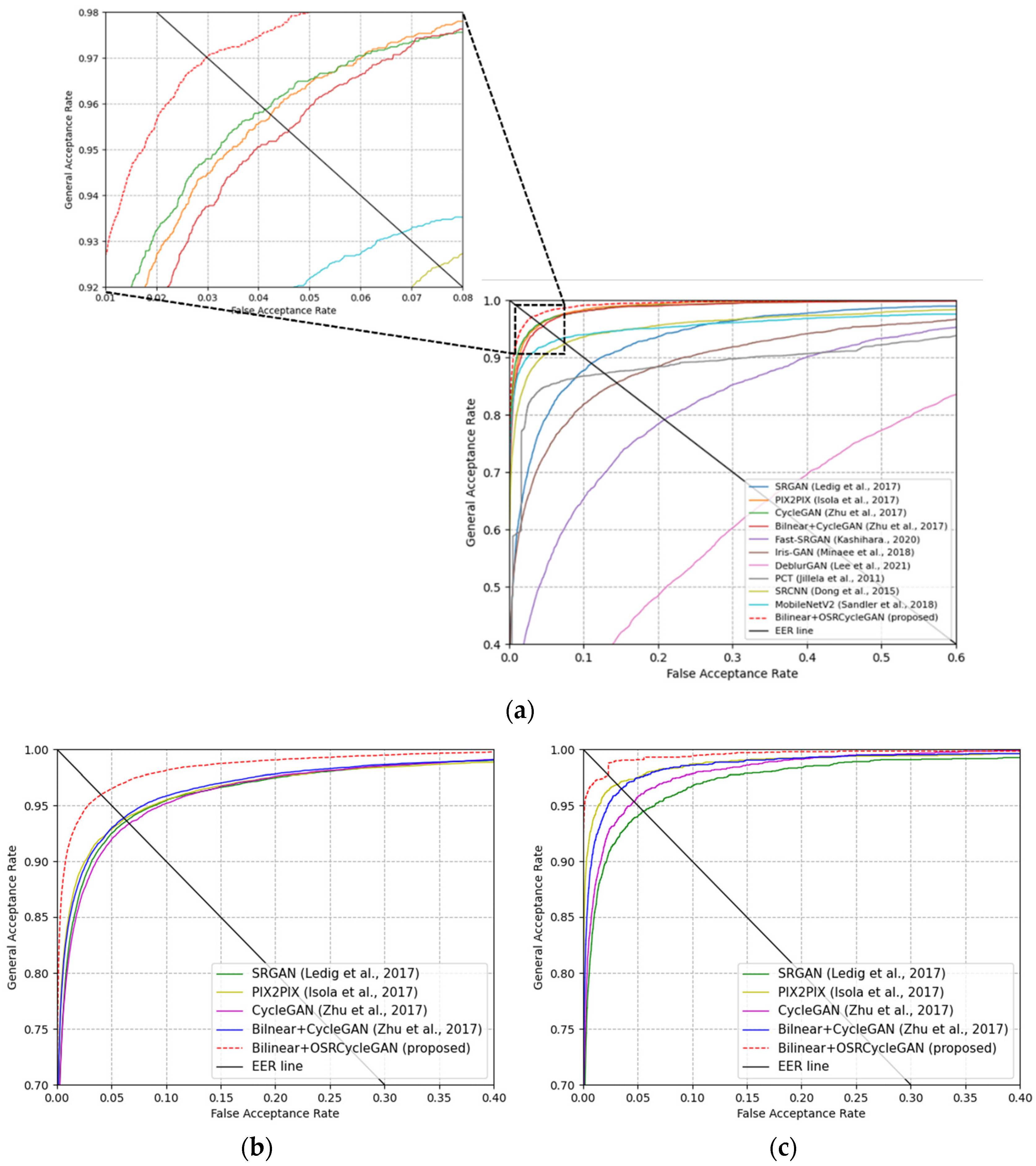
4.3.2. Comparisons with the State-of-the-Art Methods

For the next experiment, ocular recognition accuracy was compared between the proposed method and state-of-the-art methods. Comparative experiment was conducted for low-resolution images as bilinear interpolation + Gaussian blurring is more frequently used [67] than only bilinear interpolation when generating a low-resolution image. Three types of open databases, CASIA-Iris-Distance, CASIA-Iris-Lamp, and IIT Delhi iris databases were experimented; as shown in Table 8, Table 9 and Table 10, the proposed method exhibited the highest ocular recognition accuracies in all cases.
The reason why Fast-SRGAN [68] shows much higher EER compared to our method is that Fast-SRGAN was used for SR of visible-light iris images which have different image characteristics (i.e., more noises, reflections, and shadow, etc.) from those of near-infrared light images used in our experiments. The reason why Iris-GAN [69] shows much higher EER compared to our method is that Iris-GAN was based on DCGAN which generates images from random noises instead of images, and the goal of Iris-GAN is not SR but image generation for the increment of training data. The reason why DeblurGAN [70] shows much higher EER compared to our method is that DeblurGAN was used for image deblurring instead of SR. As shown in Table 8, proposed OSRCycleGAN outperforms all the traditional, learning-based, and depth-based methods.
Table 8. Comparisons with the state-of-the-art methods with CASIA-Iris-Distance database (using bilinear interpolation + Gaussian blurring when generating a low-resolution image). For the training of recognizer, train from scratch was used.
High-Resolution Image Obtained byRecognizer InputLoss for GANEER (%)
Traditional image processing-basedPCT [71]Reconstruction image
(three channels)
Null13.23
Learning-basedSRCNN [16]Mean Squared
Error loss
7.54
Deep learning-basedMobileNetV2 [72]Mean Squared
Error loss
6.78
SRGAN [19]Original
SRGAN loss
11.18
Pix2Pix [66]Original
Pix2pix loss
4.21
CycleGAN [50]Original
CycleGAN loss
4.19
Bilinear interpolation + CycleGAN [50]Interpolated image
(two channels) + reconstruction image
(one channel)
Original
CycleGAN loss
4.41
Fast-SRGAN [68]Reconstruction image
(three channel)
Original
Fast-SRGAN loss +
VGG content loss
20.86
Iris-GAN [69]Original
Iris-GAN loss
14.43
DeblurGAN [70]Original
DeblurGAN loss
34.86
Bilinear interpolation +OSRCycleGAN
(proposed)
Interpolated image
(two channels) + reconstruction image
(one channel)
Cycle
consistent loss +
Perceptual loss
3.02
Table 9. Comparisons with state-of-the-art methods with the CASIA-Iris-Lamp database (using bilinear interpolation + Gaussian blurring when generating a low-resolution image). For the training of recognizer, train from scratch was used.
High-Resolution Image Obtained byRecognizer InputLoss for GANEER (%)
SRGAN [19]Reconstruction image
(three channels)
Original
SRGAN loss
6.39
Pix2Pix [66]Reconstruction image
(three channels)
Original
Pix2pix loss
6.24
CycleGAN [50]Reconstruction image
(three channels)
Original
CycleGAN loss
6.65
Bilinear interpolation + CycleGAN [50]Interpolated image
(two channels) + reconstruction image
(one channel)
Original
CycleGAN loss
6.11
Bilinear interpolation + OSRCycleGAN
(proposed)
Interpolated image
(two channels) + reconstruction image
(one channel)
Cycle
consistent loss +
Perceptual loss
4.06
Table 10. Comparisons with state-of-the-art methods with the IIT Delhi iris database (using bilinear interpolation + Gaussian blurring when generating a low-resolution image). For the training of recognizer, train from scratch was used.
High-Resolution Image Obtained byRecognizer InputLoss for GANEER (%)
SRGAN [19]Reconstruction image
(three channels)
Original
SRGAN loss
5.57
Pix2Pix [66]Reconstruction image
(three channels)
Original
Pix2pix loss
3.09
CycleGAN [50]Reconstruction image
(three channels)
Original
CycleGAN loss
4.46
Bilinear interpolation + CycleGAN [50]Interpolated image
(two channels) + reconstruction image
(one channel)
Original
CycleGAN loss
3.35
Bilinear interpolation + OSRCycleGAN
(proposed)
Interpolated image
(two channels) + reconstruction image
(one channel)
Cycle
consistent loss + Perceptual loss
2.13
For hypothesis tests, we conducted an additional experiments of the t-test [73] and test of Cohen’s d-value [74] about the accuracies by proposed method and second best method in Table 8, Table 9 and Table 10. If the p-value by t-test is less than 0.01, it means that the null hypothesis (that two observations (the accuracies by proposed method and second best method in our case) does not show the difference) is rejected and there is a significant difference between the two observations based on 99% significant level. If the p-value is larger than 0.01 and less than 0.05, it means that there is a significant difference between the two observations based on 95% significant level [73]. Cohen’s d-value larger than 0.8 means the large effect size of the significant difference between the two observations (the accuracies proposed method and second best method in our case) [74]. Firstly, we calculated the p-value and Cohen’s d-value in Table 8. The results were 0.01274 and 6.279, respectively. For Table 9, the p-value and Cohen’s d-value were 0.01317 and 6.126, respectively. For Table 10, we got 0.02957 and 4.196, respectively. From these results, we confirm that our method shows the higher accuracies than the second best method in Table 8, Table 9 and Table 10 based on 95% significant level and large effect size.
Figure 6a–c show the receiver operating characteristic (ROC) curve of the measured recognition accuracy presented in Table 8, Table 9 and Table 10. The genuine acceptance rate is calculated as 1-FRR. Each graph is the average of the two graphs found through twofold cross-validations. As shown in Figure 6, the proposed method had the highest ocular recognition accuracies in all cases.
Figure 7 shows the examples of correct recognition cases by the proposed method. As shown in Figure 7, recognition was correctly executed even if there are differences between registered image and recognition image. That is because recognition is attempted using features extracted through a deep learning model rather than just using pixel information of the image.
Figure 8 shows the examples of false rejection and false acceptance cases by the proposed method. As shown in Figure 8, in case that recognition and enrolled images are quite similar, a false acceptance case may occur like (a) and (b), or an image belonging to the same class may not be recognized because it is restored incorrectly during restoration like (c)–(f).

4.3.3. Evaluation Based on Cross-Database Matching Performance

As next experiment, we evaluated cross-database matching performance to validate the generalization capability of the proposed method. As the 1st experiment, we performed the training of our OSRCycleGAN for SR and ResNet-101 for ocular recognition with CASIA-Iris-Lamp database, and testing with CASIA-Iris-Distance database (case 1). As the 2nd experiment, we performed the training of OSRCycleGAN and ResNet-101 with CASIA-Iris-Distance database, and testing with CASIA-Iris-Lamp database (case 2). As shown in Table 11 and Figure 9, we confirm that the recognition accuracies by cross-database matching are not much reduced compared to those by same database matching of Table 8 and Table 9, and Figure 6a,b, which validates the generalization capability of the proposed method.

4.3.4. Processing Time and System Complexity

For the last experiment, as shown in Table 12, the processing speed of the proposed method was compared in a desktop computer, as explained in Section 4.1 and in the Jetson TX2-embedded system, shown in Figure 10. The Jetson TX2-embedded system is widely used for on-board deep learning processing. Jetson TX2 has NVIDIA PascalTM-family GPU (256 CUDA cores), having 8 GB of memory shared between the central processing unit (CPU) and GPU and 59.7 GB/s of memory bandwidth; it uses less than 7.5 W of power [75]. As presented in Table 13, the proposed OSRCycleGAN had a faster processing speed than the original CycleGAN and Pix2Pix in which the proposed method had a processing speed of 145 frames/sec (1000/6.89) on a desktop computer and 9.1 frames/sec (1000/110) on the Jetson TX2-embedded system. The Jetson TX2-embedded system has limited processing power such as a number of GPU cores, thus having a slower processing speed than the desktop computer, but the proposed method was still executable.
In addition, we compared the number of floating point operations per second (#FLOPS) of Pix2Pix and CycleGAN with proposed OSRCycleGAN. As shown in Table 14, proposed OSRCycleGAN shows the better performance in #FLOPS compared to Pix2Pix. In addition, as shown in Table 13, Table 14 and Table 15, we confirm that the system complexity (#FLOPS), memory usage, and processing time by OSRCycleGAN are much less than those by CycleGAN.

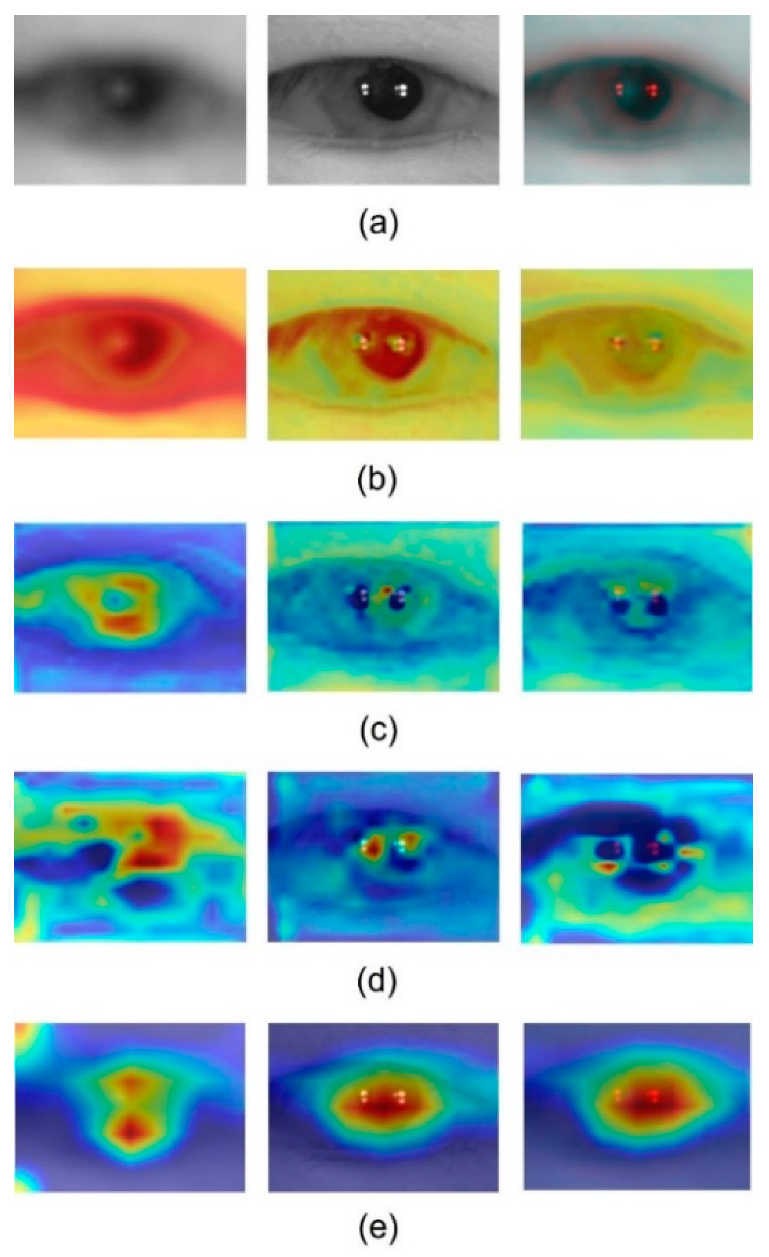
4.4. Analysis with Class Activation Maps

In this section, to determine whether the features useful for ocular recognition are extracted adequately in ResNet-101 layers for which the images restored by OSRCycleGAN are used as input, a gradient class activation map (Grad-CAM) [76] was extracted, as shown in Figure 11.
As shown in Figure 11b,c, weight is reflected in the pupil, iris region, and periocular region in the layer before the ResNet-101. Furthermore, a higher weight was reflected in the ocular region toward the subsequent layers, as shown in Figure 11d,e. Compared to low-resolution images, a higher weight was trained in the iris region in images restored to higher resolution, resulting in better recognition performance.

5. Conclusions

Existing iris or ocular recognition systems have a problem of capturing low-quality images due to low resolution; low-quality images with a blur are generated due to the movement of users when images are acquired from a far distance or low-resolution images are captured when low-priced camera equipment is used. To address these drawbacks, the study proposed an OSRCycleGAN-based SRR method. It also proposed a method for enhancing the recognition accuracy of low-resolution ocular image. When the experiments were conducted using three types of open databases, the proposed method exhibited more outstanding SRR and ocular recognition performance than state-of-the-art methods. Moreover, OSRCycleGAN had a faster processing speed than the conventional CycleGAN in a desktop computer and the Jetson TX2-embedded system, but it was still executable in an embedded system with limited processing power. The results of analyzing class activation maps showed that effective features were extracted more adequately from the images restored to high resolution using the proposed method than from low-resolution images.
Although the two loss functions (cycle consistent loss and perceptual loss) used in this method are not proposed by us, we propose a new method for calculating the perceptual loss based on both authentic and imposter matching distances between mini-batch unit images. As shown in Table 8, Table 9 and Table 10, our OSRCycleGAN using cycle consistent loss, perceptual loss, and adversarial (discriminator) loss shows the higher accuracies of ocular recognition than the original CycleGAN using cycle consistent loss, identity loss, and adversarial (discriminator) loss, which confirms the superiority of using perceptual loss instead of identity loss. Because authentic matching (matching from same class) and imposter matching (matching from different classes) should be considered as important factor in biometric system including ocular recognition, the perceptual loss based on these two matching could enhance the accuracy by our OSRCycleGAN compared to CycleGAN which does not consider the two matching even with less number of filters, system complexity, memory usage, and processing time. In addition, the identity loss of CycleGAN cannot avoid performance degradation from various effects such as pixel shifting because it just calculates the pixel differences between two images. Therefore, the identity loss was not used in our OSRCycleGAN, and we compensate the gap that comes from removing the identity loss by adding perceptual loss. These are also our innovative points compared to CycleGAN.
As shown in Table 13, proposed OSRCycleGAN shows the processing speed faster than the second best one (CycleGAN) by about 322% and 161% in desktop computer and Jetson TX2 embedded system, respectively. In addition, proposed OSRCycleGAN shows much lower number (15.3%) of #FLOPS than that by the second best one (CycleGAN) as shown in Table 14. Although the EER by our OSRCycleGAN is not much reduced compared to the second best method as shown in Table 8, Table 9 and Table 10 and Figure 6, the proportions of EER reduction by our OSRCycleGAN are 27.9% ((4.19 − 3.02)/4.19), 33.6% ((6.11 − 4.06)/6.11), and 31.1% ((3.09 − 2.13)/3.09) compared to the second best method in Table 8, Table 9 and Table 10, respectively. Because OSRCycleGAN is the enhanced model of original CycleGAN, if we compare OSRCycleGAN with the original CycleGAN having same input, the proportions of EER reduction by OSRCycleGAN are 31.5% ((4.41 − 3.02)/4.41), 33.6% ((6.11 − 4.06)/6.11), and 36.4% ((3.35 − 2.13)/3.35) compared to the original CycleGAN having same input in Table 8, Table 9 and Table 10, respectively.
In future work, the applicability of OSRCycleGAN in face recognition or vein recognition, which are other biometrics modality and person re-identification, will be analyzed. Furthermore, a lighter OSRCycleGAN model will be researched for improving the processing speed in embedded systems.

Author Contributions

Methodology, Y.W.L.; conceptualization, J.S.K.; supervision, K.R.P.; writing—original draft, Y.W.L.; writing—editing and review, K.R.P. All authors have read and agreed to the published version of the manuscript.

Funding

This research was supported in part by the National Research Foundation of Korea (NRF) funded by the Ministry of Science and ICT (MSIT) through the Basic Science Research Program (NRF-2021R1F1A1045587), in part by the NRF funded by the MSIT through the Basic Science Research Program (NRF-2022R1F1A1064291), and in part by the NRF funded by the MSIT through the Basic Science Research Program (NRF-2020R1A2C1006179).

Institutional Review Board Statement

Not applicable.

Informed Consent Statement

Not applicable.

Data Availability Statement

Not applicable.

Conflicts of Interest

The authors declare no conflict of interest.

References

  1. Proenca, H.; Neves, J.C. Deep-PRWIS: Periocular recognition without the iris and sclera using deep learning frameworks. IEEE Trans. Inf. Forensics Secur. 2017, 13, 888–896. [Google Scholar] [CrossRef] [Green Version]
  2. Noh, K.J.; Choi, J.; Hong, J.S.; Park, K.R. Finger-vein recognition based on densely connected convolutional network using score-level fusion with shape and texture images. IEEE Access 2020, 8, 96748–96766. [Google Scholar] [CrossRef]
  3. Daugman, J.G. High confidence visual recognition of persons by a test of statistical independence. IEEE Trans. Pattern Anal. Mach. Intell. 1993, 15, 1148–1161. [Google Scholar] [CrossRef] [Green Version]
  4. Daugman, J.G. Biometric Personal Identification System Based on Iris Analysis. U.S. Patent 5291560, 1 March 1994. [Google Scholar]
  5. Daugman, J.G. Statistical richness of visual phase information: Update on recognizing persons by iris patterns. Int. J. Comput. Vis. 2001, 45, 25–38. [Google Scholar] [CrossRef]
  6. Daugman, J.G. The importance of being random: Statistical principles of iris recognition. Pattern Recognit. 2003, 36, 279–291. [Google Scholar] [CrossRef] [Green Version]
  7. Daugman, J.G. How iris recognition works. IEEE Trans. Circuits Syst. Video Technol. 2004, 14, 21–30. [Google Scholar] [CrossRef]
  8. Daugman, J.G. New methods in iris recognition. IEEE Trans. Syst. Man, Cybern. Part B (Cybern.) 2007, 37, 1167–1175. [Google Scholar] [CrossRef] [Green Version]
  9. Nguyen, K.; Fookes, C.; Jillela, R.; Sridharan, S.; Ross, A. Long range iris recognition: A survey. Pattern Recognit. 2017, 72, 123–143. [Google Scholar] [CrossRef]
  10. Verma, S.; Mittal, P.; Vatsa, M.; Singh, R. At-a-distance person recognition via combining ocular features. In Proceedings of the IEEE International Conference on Image Processing, Phoenix, AZ, USA, 25–28 September 2016; pp. 3131–3135. [Google Scholar]
  11. Bharadwaj, S.; Bhatt, H.S.; Vasta, M.; Singh, R. Periocular biometrics: When iris recognition fails. In Proceedings of the 4th IEEE International Conference on Biometrics: Theory, Application, and Systems, Washington, DC, USA, 27–29 September 2010; pp. 1–6. [Google Scholar]
  12. Su, H.; Tang, L.; Wu, Y.; Tretter, D.; Zhou, J. Spatially adaptive block-based super-resolution. IEEE Trans. Image Process. 2011, 21, 1031–1045. [Google Scholar] [CrossRef]
  13. Babacan, S.D.; Molina, R.; Katsaggelos, A.K. Variational Bayesian super resolution. IEEE Trans. Image Process. 2011, 20, 984–999. [Google Scholar] [CrossRef]
  14. Hu, J.; Wu, X.; Zhou, J. Noise robust single image super-resolution using a multiscale image pyramid. Signal Process. 2018, 148, 157–171. [Google Scholar] [CrossRef]
  15. Taniguchi, K.; Ohashi, M.; Han, X.-H.; Iwamoto, Y.; Sasatani, S.; Chen, Y.-W. Example-based super-resolution using locally linear embedding. In Proceedings of the 6th International Conference on Computer Sciences and Convergence Information Technology, Jeju Island, Korea, 29 November 2011–1 December 2011; pp. 861–865. [Google Scholar]
  16. Dong, C.; Loy, C.C.; He, K.; Tang, X. Image super-resolution using deep convolutional networks. IEEE Trans. Pattern Anal. Mach. Intell. 2016, 38, 295–307. [Google Scholar] [CrossRef] [PubMed] [Green Version]
  17. Kim, J.; Lee, J.K.; Lee, K.M. Accurate image super-resolution using very deep convolutional networks. In Proceedings of the IEEE Conference on Computer Vision and Pattern Recognition, Las Vegas, NV, USA, 27-30 June 2016; pp. 1646–1654. [Google Scholar]
  18. Goodfellow, I.J.; Pouget-Abadie, J.; Mirza, M.; Xu, B.; Warde-Farley, D.; Ozair, S.; Courville, A.; Bengio, Y. Generative adversarial nets. In Proceedings of the 28th Conference on Neural Information Processing Systems, Montreal, QC, Canada, 8–13 December 2014; pp. 2672–2680. [Google Scholar]
  19. Ledig, C.; Theis, L.; Huszár, F.; Caballero, J.; Cunningham, A.; Acosta, A.; Aitken, A.P.; Tejani, A.; Totz, J.; Wang, Z.; et al. Photo-Realistic Single Image Super-Resolution Using a Generative Adversarial Network. In Proceedings of the 2017 IEEE Conference on Computer Vision and Pattern Recognition (CVPR), Honolulu, HI, USA, 21–26 July 2017. [Google Scholar]
  20. Tan, C.-W.; Kumar, A. Accurate iris recognition at a distance using stabilized iris encoding and Zernike moments phase features. IEEE Trans. Image Process. 2014, 23, 3962–3974. [Google Scholar] [CrossRef]
  21. Nguyen, K.; Fookes, C.; Sridharan, S.; Denman, S. Quality-driven super-resolution for less constrained iris recognition at a distance and on the move. IEEE Trans. Inf. Forensics Secur. 2011, 6, 1248–1258. [Google Scholar] [CrossRef]
  22. Rodriguez, A.; Panza, J.; Kumar, B.V.K.V. Segmentation-free ocular detection and recognition. In Proceedings of the SPIE Defense, Security, and Sensing, Orlando, FL, USA, 25–29 April 2011; p. 8029. [Google Scholar] [CrossRef]
  23. Cho, S.R.; Nam, G.P.; Shin, K.Y.; Nguyen, D.T.; Pham, T.D.; Lee, E.C.; Park, K.R. Periocular-based biometrics robust to eye rotation based on polar coordinates. Multimedia Tools Appl. 2015, 76, 11177–11197. [Google Scholar] [CrossRef]
  24. Oishi, S.; Ichino, M.; Yoshiura, H. Fusion of iris and periocular user authentication by AdaBoost for mobile devices. In Proceedings of the IEEE International Conference on Consumer Electronics, Las Vegas, NV, USA, 9–12 January 2015; pp. 428–429. [Google Scholar] [CrossRef]
  25. Tan, C.-W.; Kumar, A. Towards online iris and periocular recognition under relaxed imaging constraints. IEEE Trans. Image Process. 2013, 22, 3751–3765. [Google Scholar] [CrossRef]
  26. Gangwar, A.; Joshi, A. DeepIrisNet: Deep iris representation with applications in iris recognition and cross-sensor iris recognition. In Proceedings of the IEEE International Conference on Image Processing, Phoenix, AZ, USA, 25–28 September 2016; pp. 2301–2305. [Google Scholar] [CrossRef]
  27. Lee, M.B.; Gil Hong, H.; Park, K.R. Noisy ocular recognition based on three convolutional neural networks. Sensors 2017, 17, 2933. [Google Scholar] [CrossRef]
  28. Liu, M.; Zhou, Z.; Shang, P.; Xu, D. Fuzzified image enhancement for deep learning in iris recognition. IEEE Trans. Fuzzy Syst. 2019, 28, 92–99. [Google Scholar] [CrossRef]
  29. Vizoni, M.V.; Marana, A.N. Ocular recognition using deep features for identity authentication. In Proceedings of the International Conference on System, Signals and Image Processing, Niteroi, Brazil, 1–3 July 2020; pp. 155–160. [Google Scholar]
  30. Lee, Y.W.; Kim, K.W.; Hoang, T.M.; Arsalan, M.; Park, K.R. Deep residual CNN-based ocular recognition based on rough pupil detection in the images by NIR camera sensor. Sensors 2019, 19, 842. [Google Scholar] [CrossRef] [Green Version]
  31. Nguyen, K.; Fookes, C.; Sridharan, S.; Denman, S. Feature-domain super-resolution for iris recognition. Comput. Vis. Image Underst. 2013, 117, 1526–1535. [Google Scholar] [CrossRef] [Green Version]
  32. Deshpande, A.; Patavardhan, P.P.; Rao, D.H. Super-resolution for iris feature extraction. In Proceedings of the IEEE Inter-national Conference on Computational Intelligence and Computing Research, Coimbatore, India, 18–20 December 2014; pp. 1–4. [Google Scholar]
  33. Nguyen, K.; Fookes, C.; Sridharan, S.; Denman, S. Focus-score weighted super-resolution for uncooperative iris recognition at a distance and on the move. In Proceedings of the 25th International Conference of Image and Vision Computing New Zealand, Queenstown, New Zealand, 8–9 November 2010; pp. 1–8. [Google Scholar] [CrossRef] [Green Version]
  34. Fahmy, G. Super-resolution construction of iris images from a visual low resolution face video. In Proceedings of the 9th International Symposium on Signal Processing and Its Applications, Sharjah, United Arab Emirates, 12–15 February 2007; pp. 1–4. [Google Scholar]
  35. Shirke, S.D.; Rajabhushnam, C. Biometric personal iris recognition from an image at long distance. In Proceedings of the 3rd International Conference on Trends in Electronics and Informatics, Tirunelveli, India, 23–25 April 2019; pp. 560–565. [Google Scholar]
  36. Cui, J.; Wang, Y.; Huang, J.Z.; Tan, T.; Sun, Z. An iris image synthesis method based on PCA and super-resolution. In Proceedings of the 17th International Conference on Pattern Recognition, Cambridge, UK, 26 August 2004; pp. 471–474. [Google Scholar]
  37. Shin, K.Y.; Park, K.R.; Kang, B.J.; Park, S.J. Super-resolution method based on multiple multi-layer perceptrons for iris recognition. In Proceedings of the 4th International Conference on Ubiquitous Information Technologies & Applications, Fukuoka, Japan, 20–22 December 2009; pp. 1–5. [Google Scholar]
  38. Shin, K.Y.; Kang, B.J.; Park, K.R.; Shin, J.-h. A Study on the restoration of a low-resolution iris image into a high-resolution one based on multiple multi-layered perceptrons. J. Korea Multimed. Soc. 2010, 13, 1581–1592. [Google Scholar]
  39. Shin, K.Y.; Kang, B.J.; Park, K.R. Super-resolution iris image restoration based on multiple MLPs and CLS filter. J. Internet Technol. 2012, 13, 233–244. [Google Scholar]
  40. Alonso-Fernandez, F.; Farrugia, R.A.; Bigun, J. Eigen-patch iris super-resolution for iris recognition improvement. In Proceedings of the 23rd European Signal Processing Conference (EUSIPCO), Nice, France, 31 August–4 September 2015; pp. 76–80. [Google Scholar] [CrossRef] [Green Version]
  41. Ribeiro, E.; Uhl, A.; Alonso-Fernandez, F.; Farrugia, R.A. Exploring deep learning image super-resolution for iris recognition. In Proceedings of the 25th European Signal Processing Conference (EUSIPCO), Kos, Greece, 28 August 2017–2 September 2017. [Google Scholar] [CrossRef] [Green Version]
  42. Reddy, N.; Noor, D.F.; Li, Z.; Derakhshani, R. Multi-frame super resolution for ocular biometrics. In Proceedings of the IEEE/CVF Conference on Computer Vision and Pattern Recognition Workshops, Salt Lake City, UT, USA, 18–22 June 2018; pp. 566–574. [Google Scholar]
  43. Ribeiro, E.; Uhl, A. Exploring Texture Transfer Learning via Convolutional Neural Networks for Iris Super Resolution. In Proceedings of the International Conference of the Biometrics Special Interest Group (BIOSIG), Darmstadt, Germany, 20–22 September 2017. [Google Scholar] [CrossRef]
  44. Tan, J.; Liao, X.; Liu, J.; Cao, Y.; Jiang, H. Channel attention image steganography with generative adversarial networks. IEEE Trans. Netw. Sci. Eng. 2021, 9, 888–903. [Google Scholar] [CrossRef]
  45. Liao, X.; Yu, Y.; Li, B.; Li, Z.; Qin, Z. A new payload partition strategy in color image steganography. IEEE Trans. Circuits Syst. Video Technol. 2019, 30, 685–696. [Google Scholar] [CrossRef]
  46. Liao, X.; Yin, J.; Chen, M.; Qin, Z. Adaptive payload distribution in multiple images steganography based on image texture features. IEEE Trans. Dependable Secur. Comput. 2022, 19, 897–911. [Google Scholar] [CrossRef]
  47. Yin, G.; Wang, W.; Yuand, Z.; Ji, W.; Yue, D.; Sun, S.; Chua, T.-S.; Wang, C. Conditional hyper-network for blind super-resolution with multiple degradations. IEEE Trans. Image Process. 2022, 31, 3949–3960. [Google Scholar] [CrossRef]
  48. Martins, A.L.D.; Homem, M.R.P.; Mascarenhas, N.D.A. Super-resolution Image reconstruction using the ICM Algorithm. In Proceedings of the IEEE International Conference on Image Processing, San Antonio, TX, USA, 16–19 September 2007; pp. 1–4. [Google Scholar]
  49. Han, Y.; Shu, F.; Zhang, Q. Image super-resolution reconstruction based on adaptive interpolation norm regularization. In Proceedings of the International Symposium on Intelligent Signal Processing and Communication Systems, Xiamen, China, 28 November–1 December 2007; pp. 1–4. [Google Scholar]
  50. Zhu, J.-Y.; Park, T.; Isola, P.; Efros, A.A. Unpaired image-to-image translation using cycle-consistent adversarial networks. In Proceedings of the IEEE International Conference on Computer Vision, Venice, Italy, 22–29 October 2017; pp. 2242–2251. [Google Scholar]
  51. He, K.; Zhang, X.; Ren, S.; Sun, J. Deep residual learning for image recognition. In Proceedings of the IEEE Conference on Computer Vision and Pattern Recognition, Las Vegas, NV, USA, 26 June 2016; pp. 770–778. [Google Scholar]
  52. Deng, J.; Dong, W.; Socher, R.; Li, L.-J.; Li, K.; Fei-Fei, L. ImageNet: A large-scale hierarchical image database. In Proceedings of the IEEE Conference on Computer Vision and Pattern Recognition, Miami, FL, USA, 20–25 June 2009; pp. 248–255. [Google Scholar]
  53. Nair, V.; Hinton, G.E. Rectified linear units improve restricted Boltzmann machines. In Proceedings of the 27th International Conference on Machine Learning, Haifa, Israel, 21–24 June 2010; pp. 807–814. [Google Scholar]
  54. Multinomial Logistic Loss. Available online: http://caffe.berkeleyvision.org/doxygen/classcaffe_1_1MultinomialLogisticLossLayer.html (accessed on 1 July 2022).
  55. CASIA-iris Version 4. Available online: http://biometrics.idealtest.org/dbDetailForUser.do?id=4#/datasetDetail/4 (accessed on 3 July 2022).
  56. Kumar, A.; Passi, A. Comparison and combination of iris matchers for reliable personal authentication. Pattern Recognit. 2010, 43, 1016–1026. [Google Scholar] [CrossRef]
  57. Krizhevsky, A.; Sutskever, I.; Hinton, G.E. Imagenet classification with deep convolutional neural networks. In Proceedings of the 25th International Conference on Neural Information Processing Systems, Lake Tahoe, NV, USA, 3–8 December 2012; pp. 1097–1105. [Google Scholar]
  58. NVIDIA GeForce GTX 1070. Available online: https://www.nvidia.com/en-us/geforce/products/10series/geforce-gtx-1070/ (accessed on 3 July 2022).
  59. Abadi, M.; Agarwal, A.; Barham, P.; Brevdo, E.; Chen, Z.; Citro, C.; Corrado, G.S.; Davis, A.; Dean, J.; Devin, M.; et al. TensorFlow: Large-Scale Machine Learning on Heterogeneous Systems. 2015. Available online: https://www.tensorflow.org (accessed on 10 July 2022).
  60. Jia, Y.; Shelhamer, E.; Donahue, J.; Karayev, S.; Long, J.; Girshick, R.; Guadarrama, S.; Darrell, T. Caffe: Convolutional architecture for fast feature embedding. In Proceedings of the 22nd ACM International Conference on Multimedia, Orlando, FL, USA, 3–7 November 2014; pp. 675–678. [Google Scholar]
  61. Kingma, D.P.; Ba, J. Adam: A method for stochastic optimization. In Proceedings of the International Conference on Learning Representation, San Diego, CA, USA, 7–9 May 2015; pp. 1–15. [Google Scholar]
  62. Bottou, L. Stochastic Gradient Descent Tricks. In Neural Networks: Tricks of the Trade; Montavon, G., Orr, G.B., Müller, K.R., Eds.; Lecture Notes in Computer Science; Springer: Berlin, Heidelberg, 2012; p. 7700. [Google Scholar]
  63. Stathaki, T. Image Fusion: Algorithms and Applications; Academic Press: Cambridge, MA, USA, 2008. [Google Scholar]
  64. Salomon, D. Data Compression: The Complete Reference, 4th ed.; Springer: New York, NY, USA, 2006. [Google Scholar]
  65. Wang, Z.; Bovik, A.; Sheikh, H.; Simoncelli, E. Image quality assessment: From error visibility to structural similarity. IEEE Trans. Image Process. 2004, 13, 600–612. [Google Scholar] [CrossRef] [Green Version]
  66. Isola, P.; Zhu, J.-Y.; Zhou, T.; Efros, A.A. Image-to-image translation with conditional adversarial networks. In Proceedings of the IEEE Conference on Computer Vision and Pattern Recognition, Honolulu, HI, USA, 21–26 July 2017; pp. 1125–1134. [Google Scholar]
  67. Gonzalez, R.C.; Woods, R.E. Digital Image Processing; Prentice Hall: Upper Saddle River, NJ, USA, 2010. [Google Scholar]
  68. Kashihara, K. Iris recognition for biometrics based on CNN with super-resolution GAN. In Proceedings of the IEEE Conference on Evolving and Adaptive Intelligent Systems, Bari, Italy, 27–29 May 2020; pp. 1–6. [Google Scholar]
  69. Minaee, S.; Abdolrashidi, A. Iris-GAN: Learning to Generate Realistic Iris Images Using Convolutional GAN. arXiv 2018, arXiv:1812.04822. Available online: https://arxiv.org/abs/1812.04822 (accessed on 10 July 2022).
  70. Lee, M.B.; Kang, J.K.; Yoon, H.S.; Park, K.R. Enhanced Iris Recognition Method by Generative Adversarial Network-Based Image Reconstruction. IEEE Access 2021, 9, 10120–10135. [Google Scholar] [CrossRef]
  71. Jillela, R.; Ross, A.; Flynn, P.J. Information fusion in low-resolution iris videos using Principal Components Transform. In Proceedings of the IEEE Workshop on Applications of Computer Vision (WACV), Kona, HI, USA, 5–7 January 2011; pp. 262–269. [Google Scholar] [CrossRef] [Green Version]
  72. Sandler, M.; Howard, A.; Zhu, M.; Zhmoginov, A.; Chen, L.C. Mobilenetv2: Inverted residuals and linear bottlenecks. In Proceedings of the IEEE Conference on Computer Vision and Pattern Recognition, Salt Lake City, UT, USA, 18–22 June 2018; pp. 4510–4520. [Google Scholar]
  73. Student’s T-Test. Available online: https://en.wikipedia.org/wiki/Student%27s_t-test (accessed on 3 October 2022).
  74. Cohen, J. A power primer. Psychol. Bull. 1992, 112, 155. [Google Scholar] [CrossRef]
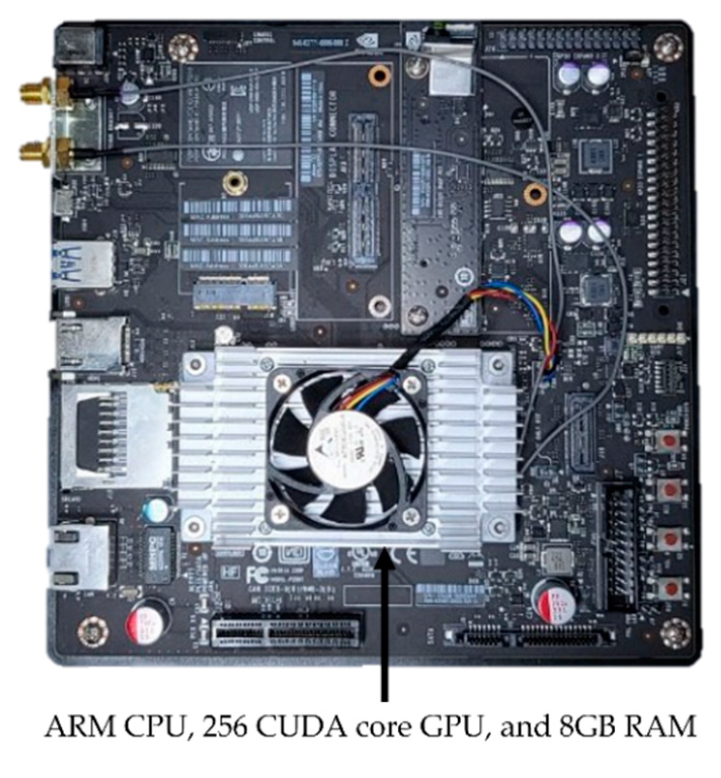
  75. Jetson TX2 Module. Available online: https://www.nvidia.com/en-us/autonomous-machines/embedded-systems/ (accessed on 15 July 2022).
  76. Selvaraju, R.R.; Cogswell, M.; Das, A.; Vedantam, R.; Parikh, D.; Batra, D. Grad-CAM: Visual Explanations from Deep Networks via Gradient-Based Localization. In Proceedings of the 2017 IEEE International Conference on Computer Vision (ICCV), Venice, Italy, 22–29 October 2017; pp. 618–626. [Google Scholar] [CrossRef]
Figure 1. Overview of the proposed method.
Mathematics 10 03818 g001
Figure 2. OSRCycleGAN. (a) Generator, (b) discriminator, and (c) whole flow of proposed method with proposed the perceptual loss calculations.
Mathematics 10 03818 g002aMathematics 10 03818 g002b
Figure 3. Graphs of training losses of generator (g_loss) and discriminator (d_loss) by OSRCycleGAN with (a) CASIA-Iris-Distance, (b) CASIA-Iris-Lamp, and (c) IIT Delhi iris databases.
Mathematics 10 03818 g003
Figure 4. Graphs of training loss and accuracy by ResNet-101 with (a) CASIA-Iris-Distance, (b) CASIA-Iris-Lamp, and (c) IIT Delhi iris databases.
Mathematics 10 03818 g004
Figure 5. Comparisons on SRR by the proposed method and the state-of-the-art methods. (a) Original high-resolution images. (b) Low-resolution images by bilinear interpolation. (c) Low-resolution images by bilinear interpolation + Gaussian blurring. (d) Output images by SRGAN with (c). (e) Output images by Pix2Pix with (c). (f) Output images by CycleGAN with (c). (g) Output images by OSRCycleGAN with (b). (h) Output images by OSRCycleGAN with (c).
Mathematics 10 03818 g005
Figure 6. ROC curves of ocular recognition by the proposed method and state-of-the-art methods with (a) CASIA-Iris-Distance, (b) CASIA-Iris-Lamp, and (c) IIT Delhi iris database.
Mathematics 10 03818 g006
Figure 7. Example of correct recognition cases by the proposed method. (a,b) CASIA-Iris-Distance database. (c,d) CASIA-Iris-Lamp database. (e,f) IIT Delhi iris database. The left-hand and right-hand side images in (af) show registered images and recognition images, respectively. 1st and 2nd row images in (af) show low-resolution and high-resolution images restored by OSRCycleGAN, respectively.
Mathematics 10 03818 g007
Figure 8. Example of recognition error cases by the proposed method. (a,b) CASIA-Iris-Distance database. (c,d) CASIA-Iris-Lamp database. (e,f) IIT Delhi iris database. (a,c,e) show false rejection cases. (b,d,f) show false acceptance cases. The left-hand and right-hand side images in (af) show registered images and recognition images, respectively. 1st and 2nd row images in (af) show low-resolution images and high-resolution images restored by OSRCycleGAN, respectively.
Mathematics 10 03818 g008
Figure 9. ROC curves of ocular recognition based on cross-database matching.
Mathematics 10 03818 g009
Figure 10. Jetson TX2 embedded system.
Mathematics 10 03818 g010
Figure 11. Grad-CAM extraction results. Each row in the figure is a low-resolution image before restoration, bilinear interpolated high-resolution image, high-resolution image after being restored by OSRCycleGAN, and when mixed images of bilinear interpolation (two channels) + OSRCycleGAN (one channel) in Table 8, Table 9 and Table 10 are used as input in the ResNet-101. (a) of each column is the input image. (b) Grad-CAM image extracted from second residual block layer, (ce) are Grad-CAM image extracted from third, fourth and fifth residual block, respectively.
Mathematics 10 03818 g011
Table 1. Comparisons of previous studies and the proposed method.
CategoryMethod(s)StrengthWeakness
Without SRRHandcrafted feature-basedIrisDaugman’s method [5,8]Does not require an additional graphics processing unitDoes not consider the performance degradation for low-resolution iris images
Stabilized iris encoding and Zernike moments phase features [20]
Noisy image captured at a distance [39]
Iris + ocularUsed ocular region including iris and periocular [10,22,23,24,25]High recognition performance in various environments as both iris and periocular region information are usedPoorer recognition performance than the deep-feature-based method
Deep
feature-based
IrisDeepIrisNet [26]Improved recognition performance for noisy iris images as multiple CNNs are usedTraining time for each model is increased as multiple CNNs are used
OcularMultiple CNN-based noisy ocular recognition [27]Solves existing iris segmentation accuracy problem and low-quality image issue by using both iris and ocular regions- Training time increases because of multiple CNNs
- Does not consider the performance degradation for low-resolution images
With SRRImage
processing-based
IrisSRR for captured image at a distance [21,33], MAP [31], PG + POCS [32], FCM [35]SRR was applied to prevent performance degradation due to low-resolution image captured from a long distanceLimitations in resolution restoration because of existing image processing technique
Learning-basedPCA + ICA [34], PCA [36,40], MLP [37,38,39]Better restoration results than traditional image processing methodsLimited improvement of SRR performance in various environments
Deep
feature-based
IrisStacked auto-encoder [41], SRCNN + VDCNN [43]Higher SRR performance than image processing-based or learning-based methodsLimited recognition and SRR accuracies in various environments as a general CNN or encoder are used
OcularMulti-frame SRR + CNN-based deblurring [42]Improved performance by separating SRR and deblurring processes
OSRCycleGAN
(proposed method)
Generator and discriminator improve SRR performance through competitive learning Requires intensive training procedure
Table 2. Generator of OSRCycleGAN (* and ** means that the BN + ReLU and Conv + BN + ReLU + Conv + BN combinations are applied after the Conv or in each residual block, respectively. BN, ReLU, and Conv mean batch normalization, rectified linear unit, and convolution layer, respectively).
LayersFeature Map Size
(Width × Height × Channels)
Filter SizeNumber of FiltersStride
Input layer380 × 280 × 3
Conv-1 *380 × 280 × 327 × 7 × 3321
Conv-2 *190 × 140 × 643 × 3 × 32642
Conv-3 *95 × 70 × 1283 × 3 × 641282
Residual 1–6 **95 × 70 × 1283 × 3 × 1281281
Deconv1 *190 × 140 × 644 × 4 × 128642
Deconv2 *380 × 280 × 324 × 4 × 64322
Output *380 × 280 × 37 × 7 × 3231
Table 3. Discriminator of OSRCycleGAN (#filter and S mean the number of filters and strides, respectively) (* and ** means that the Leaky ReLU (LReLU) and BN + LReLU combination are applied after the Conv, respectively. ReLU, BN, and Conv mean rectified linear unit, batch normalization, and convolution layer, respectively).
LayersFeature Map Size
( Width × Height × Channels )
Filter SizeNumber of FiltersStride
Input layer380 × 280 × 3
Conv-1 *190 × 140 × 324 × 4 × 3322
Conv-2 **95 × 70 × 644 × 4 × 32642
Conv-3 **48 × 35 × 1284 × 4 × 641282
Conv-4 **24 × 18 × 2564 × 4 × 1282561
Conv-5 (Output)24 × 18 × 14 × 4 × 25611
Table 4. Detailed descriptions of the experimental databases.
CategoryNumber of ClassesNumber of Images
Before AugmentationAfter Augmentation
DB1DB2DB1DB2DB1DB2
CASIA-Iris-Distance14214020802056351,520347,464
CASIA-Iris-Lamp408408805480361,361,1261,358,084
IIT Delhi iris database21022311201120189,280189,280
Table 5. Comparisons on SRR by the proposed method and state-of-the-art methods.
MethodsPSNRSNRSSIM
SRGAN [19]15.641.150.68
Pix2Pix [66]27.25.910.78
CycleGAN [50]18.41.740.71
OSRCycleGAN22.662.030.74
Table 6. Ocular recognition accuracy comparison in the case of using only bilinear interpolation when generating a low-resolution image (* means fine-tuning using the model pretrained with original high-resolution ocular images, and ** means fine-tuning using the model pretrained with ImageNet).
High-Resolution Image Obtained byRecognizer
Input
Recognizer Training MethodLoss for OSRCycleGANEER (%)
Bilinear interpolationInterpolated image
(three channels)
Without training
(only testing)
Loss is not used11.41
Fine-tuning *4.58
OSRCycleGANReconstruction image
(three channels)
Without training
(only testing)
Cycle consistent loss8.55
Cycle consistent loss + Perceptual loss11.68
Fine-tuning *Cycle consistent loss13.98
Cycle consistent loss + Perceptual loss4.28
Bilinear interpolation + OSRCycleGAN
(proposed)
Interpolated image
(two channels) + reconstruction image(one channel)
Fine-tuning *Cycle consistent loss9.26
Cycle consistent loss + Perceptual loss7.01
Fine-tuning **Cycle consistent loss13.25
Cycle consistent loss + Perceptual loss3.28
Train from scratchCycle consistent loss4.23
Cycle consistent loss + Perceptual loss3.93
Table 7. Ocular recognition accuracy comparison in the case of using bilinear interpolation + Gaussian blurring when generating a low-resolution image (* means fine-tuning using the model pretrained with original high-resolution ocular images, and ** means fine-tuning using the model pretrained with ImageNet).
High-Resolution Image Obtained byRecognizer
Input
Recognizer Training MethodLoss for OSRCycleGANEER (%)
Bilinear interpolation +
Gaussian Blurring
Interpolated
image
(three channels)
Without training
(only testing)
Loss is not used13.99
Fine-tuning *4.82
OSRCycleGANReconstruction
image
(three channels)
Without training
(only testing)
Cycle consistent loss10.84
Cycle consistent loss + Perceptual loss6.15
Fine-tuning *Cycle consistent loss13.26
Cycle consistent loss + Perceptual loss5.41
Bilinear interpolation +
OSRCycleGAN
(proposed)
Interpolated image
(two channels) + reconstruction
image(one channel)
Fine-tuning *Cycle consistent loss4.42
Cycle consistent loss + Perceptual loss3.80
Fine-tuning **Cycle consistent loss5.56
Cycle consistent loss + Perceptual loss10.69
Train from scratchCycle consistent loss6.95
Cycle consistent loss + Perceptual loss3.02
Cycle consistent loss + Perceptual loss +
Identity loss
6.26
Cycle consistent loss + Perceptual loss +
Identity loss +
Focal loss
5.88
Table 11. Evaluation based on cross-database matching performance. Case 1 means the training of OSRCycleGAN for SR and ResNet-101 for ocular recognition with CASIA-Iris-Lamp database, and testing with CASIA-Iris-Distance database. Case 2 means the training of OSRCycleGAN and ResNet-101 with CASIA-Iris-Distance database, and testing with CASIA-Iris-Lamp database.
CasesEER (%)
Case 13.68
Case 26.46
Table 12. Average processing time of one image by the proposed method (unit: ms).
EnvironmentsOSRCycleGANResNet-101Total
Desktop computer6.894753.89
Jetson TX2
embedded system
110313423
Table 13. Average processing time of one image by Pix2Pix, original CycleGAN, and proposed OSRCycleGAN (unit: ms).
EnvironmentsPix2Pix [66]CycleGAN [50]OSRCycleGAN
Desktop computer25.5322.226.89
Jetson TX2
embedded system
273177110
Table 14. Comparisons on #FLOPS of one image by Pix2Pix, original CycleGAN, and proposed OSRCycleGAN (unit: #FLOPS).
Pix2Pix [66]CycleGAN [50]OSRCycleGAN
111.6 × 10624.07 × 1063.69 × 106
Table 15. Comparisons on memory usage by CycleGAN and proposed OSRCycleGAN (unit: Giga Bytes).
CycleGAN [50]4.11
OSRCycleGAN2.04
Publisher’s Note: MDPI stays neutral with regard to jurisdictional claims in published maps and institutional affiliations.

