Survey on the Application of Artificial Intelligence in ENSO Forecasting

Abstract

Climate disasters such as floods and droughts often bring heavy losses to human life, national economy, and public safety. El Niño/Southern Oscillation (ENSO) is one of the most important inter-annual climate signals in the tropics and has a global impact on atmospheric circulation and precipitation. To address the impact of climate change, accurate ENSO forecasts can help prevent related climate disasters. Traditional prediction methods mainly include statistical methods and dynamic methods. However, due to the variability and diversity of the temporal and spatial evolution of ENSO, traditional methods still have great uncertainty in predicting ENSO. In recent years, with the rapid development of artificial intelligence technology, it has gradually penetrated into all aspects of people’s lives, and the climate field has also benefited. For example, deep learning methods in artificial intelligence can automatically learn and train from a large amount of sample data, obtain excellent feature representation, and effectively improve the performance of various learning tasks. It is widely used in computer vision, natural language processing, and other fields. In 2019, Ham et al. used a convolutional neural network (CNN) model in ENSO forecasting 18 months in advance, and the winter ENSO forecasting skill could reach 0.64, far exceeding the dynamic model with a forecasting skill of 0.5. The research results were regarded as the pioneering work of deep learning in the field of weather forecasting. This paper introduces the traditional ENSO forecasting methods and focuses on summarizing the various latest artificial intelligence methods and their forecasting effects for ENSO forecasting, so as to provide useful reference for future research by researchers.

1. Introduction

Climate change is a difficult problem facing the world today, and it affects people’s production and life to a large extent. The most prominent El Niño-Southern Oscillation (ENSO) phenomenon is the most important interannual signal of short-term climate change on the earth [1]. It will have a great impact on the climate, environment, and socio-economics on a global scale.

ENSO is wind and sea surface temperature oscillations that occur in the equatorial eastern Pacific. In 1969, Bjerknes [2] proposed that El Niño and the Southern Oscillation are two different manifestations of the same physical phenomenon in nature, which is reflected in the ocean as the El Niño phenomenon and in the atmosphere as the Southern Oscillation phenomenon. El Niño refers to the phenomenon of abnormal warming of the ocean every two to seven years (every four years on average) in the equatorial eastern Pacific Ocean, and the opposite cold phenomenon is called La Niña [3]. The Southern Oscillation refers to the mutual movement of the atmosphere between the eastern tropical Pacific and the western tropical Pacific, and the cycle is also approximately four years. El Niño and La Niña are closely related to the Southern Oscillation. When the Southern Oscillation index has a persistent negative value, an El Niño phenomenon will occur in that year, and on the contrary, a La Niña phenomenon will occur in that year.

Since ENSO is a global ocean–atmosphere interaction, it has a huge impact on crop yields, temperature, and rainfall on Earth. In 1997-1998, fires triggered by an unusual drought caused by ENSO destroyed large swathes of tropical rainforest worldwide [4]. Hurricanes caused considerable damage in the United States from 1925-1997, with an average annual loss of $5.2 billion [5]. In ENSO years, flood risk anomalies exist in basins spanning almost half of the Earth’s surface [6]. The World Health Organization estimates that over the past 30 years, anthropogenic warming and precipitation have claimed 150,000 lives each year [7]. In order to deal with the threat of such climate disasters, knowing and understanding the laws of climate change and making effective climate predictions in advance are crucial to reducing disaster losses around the world.

ENSO prediction is one of the most important issues in climate science, affecting both interannual climate predictions and decadal predictions of near-term global climate change. Since the 1980s, scientists from all over the world have been working on ENSO prediction research [8]. Since the relevant time scale of SST variability in most of the tropical Pacific Ocean is about 1 year, the ENSO event dominates the SST variability [9], and the occurrence of ENSO is reflected by the sea surface temperature anomaly (SSTA); therefore, ENSO is predicted. The phenomenon is equivalent to predicting SSTA. In addition, among all the indices, Niño3.4 is the most commonly used index to measure ENSO phenomena, and the Niño3.4 index is the mean sea temperature in the range of 5° N~5° S 170° W~120° W.

ENSO projections are by far the most successful of short-term climate predictions. Traditional ENSO prediction models are mainly divided into two categories: statistical models and dynamic models. Statistical models analyze and predict ENSO through a series of statistical methods, such as the linear transpose model (LIM), nonlinear canonical correlation analysis (NLCCA), singular spectrum analysis (SSA), etc. Essentially, this is accidental, they do not take full advantage of the laws of physics. The dynamic models are mainly based on the dynamic theory of atmosphere–ocean interaction, such as the intermediate coupled model (ICM), the hybrid coupled model (HCM), and the coupled circulation model (CGCM) [10]. It is successful in short-term prediction, but it does not make full use of the large amount of existing real historical data. For long-term prediction, the pure dynamic method is difficult to work. Practice has shown that both dynamic methods and statistical methods have a certain accuracy, and both can reflect some of the laws of atmospheric motion [11,12,13], but due to the variability and diversity of ENSO spatiotemporal evolution, traditional methods of predicting ENSO still have great deficiencies, especially in the 21st century; the intensified influence of the extratropical atmosphere on the tropics makes ENSO more complex and unpredictable.

The concept of artificial intelligence first came from the Dartmouth Conference on Computers in 1956, and its essence is to hope that machines can think and respond similarly to human brains. Machine learning is an important way to realize artificial intelligence. As the most important branch of machine learning, deep learning has developed rapidly in recent years and is now widely used in image recognition, natural language processing, and other fields.

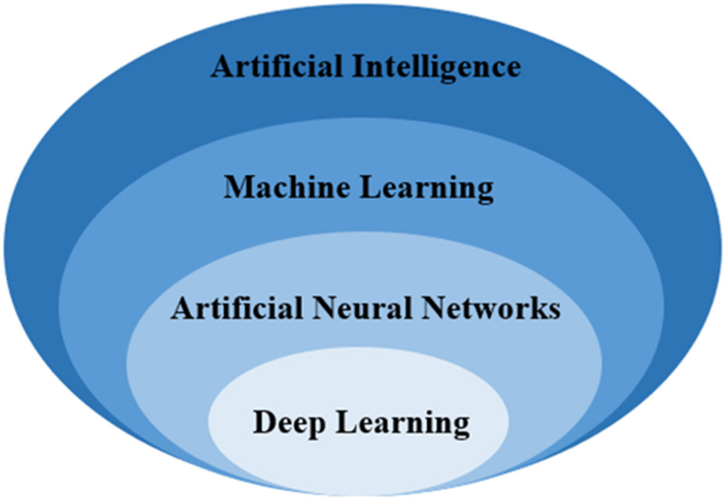
The concept of deep learning, which refers to the machine learning process of obtaining a deep network structure containing multiple levels through a certain training method based on sample data, was first proposed by Hinton et al. [14] at the University of Toronto in 2006. Figure 1 shows the relationship among artificial intelligence, machine learning, artificial neural networks and deep learning. Unlike machine learning, the deep learning feature extraction process is performed automatically through deep neural networks. The features in the neural network are obtained through learning. Under normal circumstances, when the network layer is shallow, the extracted features are less representative of the original data. When the number of network layers is deep, the features extracted by the model will be more representative. When the task to be solved is more complex, the parameter requirements of the model are also higher, and the number of network layers at this time is often deeper, which means that more complex tasks can be solved. Therefore, it can be considered that the deeper the network layer, the stronger the feature extraction ability. Currently, the commonly used deep neural network models mainly include CNN, recurrent neural network (RNN), deep belief network (DBN), and the deep autoencoder and generative adversarial network (GAN).

With the wide application of machine learning and deep learning in various fields in recent years, some scholars have begun to use machine learning or deep learning technology to predict meteorological elements (wind speed, temperature, etc.) or climate phenomena, such as ENSO, and have obtained better results. This paper will summarize the previous research results and make a more complete summary of ENSO predictions combined with deep learning.

This paper is organized as follows: Section 1 outlines the main learning knowledge and development status in ENSO forecasting; Section 2 focuses on traditional ENSO forecasting methods; Section 3 is the key part of this paper, introducing the related models and theories of deep learning in artificial intelligence and the existing ENSO prediction methods and applications of deep learning in artificial intelligence; Section 4 summarizes the ENSO forecasting methods in tabular form and discusses the existing deficiencies and future development directions of ENSO predictions; finally, Section 5 provides a summary of the full text.

2. Traditional Methods

In this section, we will focus on the existing theories or conclusions of traditional ENSO forecasting methods. There are generally two methods for traditional ENSO prediction, namely, the statistical model and the dynamic model. The following will list the currently commonly used ENSO forecast methods and related ENSO forecast knowledge.

2.1. Climate Dynamics Methods

The dynamic method uses dynamic equations to model the ocean, atmosphere, land, and other spheres and their interactions and uses the computer to gradually integrate to simulate the evolution of the atmosphere. Since the first coupled ENSO model was developed [15,16], various types of coupled models have been designed and used for ENSO simulation and prediction. The coupling models mainly include the simple coupled model (SCM) [17], intermediate coupled model (ICM) [16], hybrid coupled model (HCM) [18], and fully coupled circulation models (GCMs) [19]. Dynamical models have become the main tool for studying the mechanism, simulation, and prediction of ENSO, and the prediction time reaches 6–12 months. Ref. [17] identified several free equatorial modes for simple coupled ocean–atmosphere models and found that they included unstable and damped modes at large regional scales and long periods, systematically exploring the effects of ocean thermodynamics on the behavior of unstable modes. Ref. [16] developed an atmosphere–ocean coupled model to study the ENSO phenomenon. In the absence of anomalous external forcing, the coupled model reproduces some key features of the observed phenomenon. The results show that the mean sea surface temperature, wind, and ocean current field determine the characteristic spatial structure of the ENSO anomaly. Ref. [18] conducted a series of hindcast and prediction experiments using the HCM of the tropical ocean–atmosphere system. It shows real skills in forecasting fall/winter tropical Pacific SST up to 18 months in advance. Ref. [19] used an integrated ocean–atmosphere circulation model (OAGCM) for climate prediction. Both model performance and data assimilation schemes for climate simulations were improved to yield better forecasting skills. Most OAGCMs can now proficiently predict the Indian Ocean Dipole (IOD) 1–2 seasons in advance, with ENSOs up to 6–9 months ahead.

In recent years, many forecasting systems have been put into use. The National Climate Center of China Meteorological Administration (BCC/CMA) developed the ENSO Monitoring, Analysis and Prediction System (SEMAP2) [20]. The system consists of five subsystems: real-time monitoring of tropical atmosphere and ocean, dynamic diagnosis, physical-based statistical prediction, model ensemble prediction, and simulation-based model prediction [21] correction, which can realize the feedback process of ENSO changes and dynamics in the recent year real-time monitoring and can provide users with forecasts of the ENSO index and related main variable processes in the coming year. Since the spring of 2013, SEMAP2 has been applied to ENSO business meetings organized by the National Climate Center several consecutive times and given forecast opinions, with good results and was adopted by forecasters many times. Especially in the spring of 2014, the prediction of the evolution trend of El Niño in summer and autumn was basically in line with reality and more accurately predicted the weak central EI Nino event in the winter of 2014/15 and accurately predicted the development of El Niño since the spring of 2015. Trends and Type Conversions. The forecasting system is still in use to this day. The fifth-generation seasonal forecast system SEAS5 was put into use in November 2017 by the European Centre for Medium-Range Weather Forecasts. It is a coupled dynamical model that includes higher resolution models of the atmosphere, ocean, and sea ice. An important improvement in SEAS5 is the weakening of the cold tongue bias in the equatorial Pacific, while the amplitude of El Niño is closer to the actual value and improves the prediction ability of El Niño in the central and western Pacific, making it show particular advantages in ENSO predictions. When the forecast period is 9 months, the correlation coefficient of SEAS5 to ENSO forecast reaches more than 0.7 [22].

If the starting time of the prediction model is advanced by more than 6 months, the prediction ability of the traditional method model will be greatly reduced due to the phenomenon of the spring predictability barrier (SPB) [1]. The SPB phenomenon was discovered by Webster et al. [23] in the dynamic prediction model. Wang et al. [24] proposed that the largest vertical temperature gradient and the weakest east–west thermal difference in spring are conducive to the growth of the coupled system disturbance, which in turn makes the spring sea-air coupling the most unstable, which is conducive to the generation of the SPB phenomenon. Chen et al. [25] proposed a novel ENSO prediction model (EPM) that combines tropical states and extratropical ocean–atmosphere interactions, which can significantly improve ENSO forecasting skills beyond the spring-predictable barriers. Although dynamical models are successful in short-term predictions, pure dynamical methods are ineffective for long-term predictions.

2.2. Mathematical Statistical Methods

The statistical ENSO prediction method is to realize the analysis and prediction of ENSO phenomenon by sorting, summarizing, and analyzing historical ENSO indicators. Statistical models include linear statistical models and nonlinear statistical models. The former is constructed using linear methods such as multiple linear regression, canonical correlation, and Markov chains, while the latter is mainly constructed using machine learning methods such as Bayesian and neural networks.

2.2.1. Traditional Linear Statistical Methods

Among the traditional linear statistical methods, there are two outstanding classical methods, Holt Winters (HW) method and autoregressive integrated moving average (ARIMA) method. The HW method is a short-term statistical method [26] that proposes a forecasting expression for exponentially weighted moving averages for forecasting time series with seasonal patterns and repeating forms, using a technique called “exponential smoothing”, reducing the volatility of time-series data, allowing for a clearer understanding of its rationale [27]. In 2014, Mike et al. used the HW model to predict the SST index in the Niño3 region from 1933 to 2012 by 1 month and 12 months in advance, with a root mean square error of 0.303 and 1.309. To address the shortcoming that the HW model is not suitable for periodically stationary time series, they proposed an improved HW model called the dynamic seasonal model (DSM). Experiments show that this model predicts monthly Nino3 in sample analysis Area, and is better than the deterministic seasonal model and HW model in terms of sea surface temperature index and intraday stock return changes [28].

ARIMA, also known as the integrated moving average autoregressive model, is one of the time series forecasting analysis methods. In 2011, Matthieu et al. [29] developed a time-series analysis method using ARIMA to investigate the temporal correlation between monthly P. falciparum case numbers and ENSO measured by SOI at Cayenne General Hospital from 1996 to 2009. Results showed that an El Niño lag of 3 months had a positive effect on P. falciparum cases (p < 0.001), and adding SOI data to the ARIMA model reduced the Akaike information criterion (AIC) [30] by 4%. However, ARIMA cannot return estimates of seasonal components [31]. In addition, Penland et al. [32] proposed to represent the Indo-Pacific SSTAs as a stable linear process driven by spatially coherent stochastic forcing, obtain the relevant parameters that best fit the stable linear process through observations, and then make assumptions about stability and linearity. The experimental results show that the optimal model can achieve a sample correlation of 67% between two time series predicted 7 months in advance. The multiple linear regression model proposed by Tseng et al. [33] only relies on five evolutions of thermocline depth anomalies and zonal surface wind modulation over a 25-day period. It successfully post-reported all ENSOs except the 2000/01 La Niña. Xue et al. [34] established a forecast model using the linear Markov model, using sea surface temperature, sea level height, and wind stress as predictors. When the forecast period is 6 months, its forecast-related skill reaches 0.8. Kondrashov et al. [35] obtained the stochastic forcing model of ENSO by polynomial regression analysis. When the forecast period is 6 months, the correlation coefficient exceeds 0.6.

The ENSO phenomenon is a highly complex and dynamic pattern whose trend over time is nonlinear. Traditional statistical methods have poor fitting effect on nonlinear data sets, and are not ideal for complex pattern recognition and knowledge discovery.

2.2.2. Machine Learning Methods

The ML-based ENSO prediction method is realized by learning and mining historical ENSO index features and establishing an ENSO prediction model. In 1998, Tangang et al. [36] and Jiang Guorong et al. [37] found that the combination of the neural network algorithm and empirical orthogonal function analysis method can have unexpected effects on ENSO forecasting. In 2009, Silvestre and William [38] proposed two nonlinear regression models, Bayesian neural network (BNN) and support vector regression (SVR). Temperature can be used as a predictor of SST anomalies in the tropical Pacific for 3–15 months. The results show that the BNN model has better overall prediction performance than the SVR model. Liu Kefeng et al. [39] also found that the multi-step hierarchical prediction method based on the combination of support vector machine and wavelet decomposition method can effectively predict the time series of sea temperature anomalies. Feng et al. [40] proposed a toolbox “climatelearn”, combined with some machine learning methods, to predict the occurrence of El Niño and Niño3.4 indices. In 2016, in terms of ENSO forecasting, the zero-mean random error model of ICM was proposed [41], called the ensemble-mean model, which showed better results than the deterministic ICM on ENSO forecasting. Peter D et al. [42] combined the classic autoregressive synthetic moving average technique with an artificial neural network to predict the ENSO index. In addition, Li Chentong used the decision tree algorithm to establish a multi-modal ENSO prediction result intelligent consultation system. He used four decision tree model methods (boosting-based GBDT, XGBoost, lightGBM, and bagging-based RF), respectively, and established a multi-modal ENSO forecasting result intelligent consultation system according to different advance forecasting times.

ML-based methods, especially those based on deep networks, tend to be more complex, take longer to compute, and have poor predictive ability for very long sequences of ENSO indices. In addition, for the long-time series Niño 3.4 index and SOI data, they not only have approximately periodic interannual variation characteristics but also have a large amount of high-frequency random noise due to seasonal variation, which seriously reduces the predictive ability of numerical simulation models. Therefore, ENSO events are still difficult to predict with a lead time of more than one year.

3. Deep Learning Methods

With the rapid development of big data and deep learning methods in recent years, prediction methods based on deep learning have been widely used in various fields, and some scholars have begun to use deep learning to improve ENSO forecasting skills. This section mainly introduces the related models and theories of spatiotemporal sequences in deep learning and the application of deep learning in ENSO prediction, including shallow neural networks, CNNs, RNNs, and graph neural networks (GNN).

3.1. Shallow Neural Networks

In 1986, Rumelhar and Hinton [43] proposed the back-propagation algorithm, which solved the complex calculation problem of the two-layer neural network, which led to the research upsurge of the two-layer neural network in the industry. In addition to an input layer and an output layer, a two-layer neural network also includes an intermediate layer, where both the intermediate layer and the output layer are computational layers. Its matrix change formula is:

$$\left(W^{\left(1\right)}\ast a^{\left(1\right)}\right)=a^{\left(2\right)}$$

$$g\left(W^{\left(2\right)}\ast a^{\left(2\right)}\right)=z$$

(1)

In each layer of the neural network, except for the output layer, there will be a bias unit. As in linear regression models and logistic regression models. The matrix operation of the neural network after considering the bias is as follows:

$$g\left(W^{\left(1\right)}\ast a^{\left(1\right)}+b^{\left(1\right)}\right)=a^{\left(2\right)}$$

$$g\left(W^{\left(2\right)}\ast a^{\left(2\right)}+b^{\left(2\right)}\right)=z$$

(2)

Different from the single-layer neural network, it is theoretically proven that the two-layer neural network can approximate any continuous function infinitely, that is to say, in the face of complex nonlinear classification tasks, the two-layer neural network can better classify.

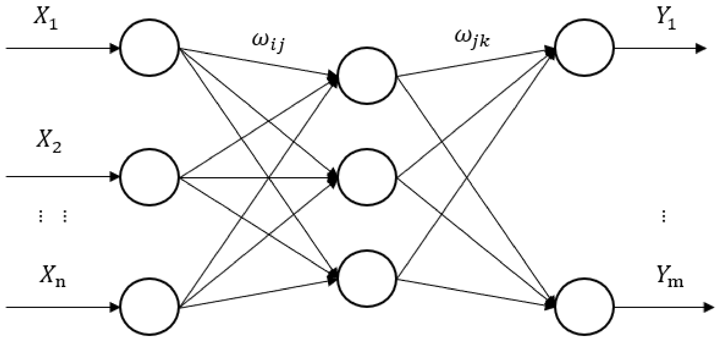
The multi-layer neural network continues to add layers after the output layer of the two-layer neural network. Its advantage is that it can represent features in a deeper way and has a stronger ability to simulate functions. The BP neural network is a concept proposed by scientists headed by Rumelhart and McClelland in 1986. It is a multi-layer feedforward neural network trained according to the error back-propagation algorithm. In other words, it is a feedforward multi-layer perceptron (MLP) trained using the BP algorithm. The BP neural network is widely used in meteorological forecasting. The classic BP neural network is generally divided into three layers, namely, the input layer, the hidden layer, and the output layer. The main idea of its training is: input data, use the back-propagation algorithm to continuously adjust and train the weights and thresholds of the network, adjust the weights and thresholds according to the prediction error, and output the results that are close to the expectations until the predicted results can reach the expectations. The topology of the BP neural network is shown in Figure 2.

When the BP neural network processes data, the network should be initialized first and the network parameters should be set; The second step is to calculate the output of the hidden layer, the output formula is shown in Formula (3), where X represents the input variable, ${\omega }_{ij},a$ are the input connection weight of the layer and the hidden layer and the threshold of the hidden layer, $l$ is the number of nodes in the hidden layer, $f$ is the activation function of the hidden layer; then the output layer is calculated, and the predicted output $Y$ of the BP network is shown in formula (4), Among them, $H$ is the output of the hidden layer, ${\omega }_{ij},b$ are the connection weights and thresholds, respectively; The formula for calculating the error is shown in (5), where $Y_k$ is the predicted value of the network, $O_k$ is the actual expected value; We update the weights and update the network connection weights ${\omega }_{ij},{\omega }_{jk}$ through the prediction error $e$. The formula is shown in (6), and $\eta$ is the learning rate; the network thresholds a and b are updated according to the prediction error e, and the formula is shown in (7); Finally, determine whether the iteration can end. If the algorithm iteration does not end, we return to the second step until the algorithm ends.

$$H_j=f\left({\displaystyle \sum }_{i=1}^n{\omega }_{ij}{x}_i+a_j\right), j=1,2,\dots ,l$$

(3)

$$Y_k={\displaystyle \sum }_{j=1}^l{H}_j{\omega }_{jk}+b_k, k=1,2,\dots ,m$$

(4)

$$e_k=Y_k-O_k, k=1,2,\dots ,m$$

(5)

$$\begin{array}{c}{\omega }_{ij}={\omega }_{ij}+\eta H_j\left(1-H_j\right)x_i{\displaystyle {\displaystyle \sum }_{k=1}^m}{\omega }_{jk}{e}_k, i=1,2,\dots ,n;j=1,2,\dots ,l\\ {\omega }_{jk}={\omega }_{jk}+\eta H_j{e}_k, j=1,\dots ,l;k=1,\dots ,m\end{array}$$

(6)

$$\begin{array}{c}{a}_j=a_j+\eta H_j\left(1-H\right)x_i{\displaystyle {\displaystyle \sum }_{k=1}^m}{\omega }_{jk}{e}_k, j=1,\dots ,l\\ b_k=b_k+\eta e_k, k=1,\dots ,m\end{array}$$

(7)

Many researchers initially tried to apply shallow neural networks to ENSO prediction and achieved good results. Jiang Guorong et al. [37] used the back-propagation (BP) algorithm for ENSO forecasting, which could better predict the changing trend of SST in key areas. However, forecast skill assessment depends on forecast time, which is inversely proportional. Baawain et al. [44] designed a three-layer multi-layer perceptron model, and the hidden layer and output layer were trained using a logical activation function through an error back-propagation algorithm. Ravi et al. [45] used the ANN model to select the Niño1+2, Niño3, Niño3.4, and Niño4 indices as the predictors of the Indian summer monsoon rainfall index (ISMRI) for prediction. The results show that the neural network model has better predictive power than all linear regression models. Mekanik et al. [46] found through experiments that using the lagged ENSO-DMI index combined with ANN to predict spring rainfall can achieve a 96.96% correlation. This method can be used in areas of the world where there is a relationship between rainfall and large-scale climate patterns that cannot be established by linear methods. Petersik and Dijkstra et al. [47] used an ensemble of Gaussian density neural networks and quantile regression neural networks to train ENSO indices and ocean heat content with a small amount of data to predict ENSO. For 1963–2017 assessments, these models are highly correlated with longer lead times. However, the shallow neural network has limited ability to represent complex functions, and its generalization ability for complex classification problems is restricted to a certain extent, and the shallow neural network tends to fall into a local minimum during training, which is prone to overfitting during testing. The multi-layer neural network can represent complex functions with fewer parameters by learning a deep nonlinear network structure and has strong feature learning ability. A multi-layer neural network has great potential to solve complex nonlinear stochastic problems with many influencing factors such as climate prediction.

3.2. Convolutional Neural Networks

Research on CNNs began in the 1980s and 1990s, and time delay networks and LeNet-5 were the first CNNs. Yann LeCun et al. [48] proposed a CNN algorithm based on gradient learning in 1998 and applied it to handwritten digit recognition. In 2012, Hinton et al. [49] won the classification competition, which opened the prelude to the gradual domination of CNNs in the field of computer vision.

As a type of neural network, CNN can effectively extract features contained in images, so it is widely used in fields involving image processing (such as image recognition, object detection, etc.) [49,50]. For meteorological data, the distribution field of a certain element at a certain time can be regarded as an image, and it can be used as the input of CNN. Using CNN to solve it is actually a nonlinear regression of the global ocean element field and the Nino3.4 regional SST in the next few months.

The main structure of CNN includes input layer, convolution layer, pooling layer, fully connected layer, and output layer. The main function of the convolution layer is to enhance the original signal features and reduce noise through convolution operations. The expression for convolution in calculus is:

$$S\left(t\right)=\int x\left(t-a\right)w\left(a\right)da$$

(8)

The discrete form is:

$$s\left(t\right)={\displaystyle \sum }_{a}x\left(t-a\right)\omega \left(a\right)$$

(9)

This formula can be expressed as a matrix:

$$\left(t\right)=\left(X\ast W\right)\left(t\right)$$

(10)

Among them, $\ast$ represents the convolution operation; if it is a two-dimensional convolution, it is represented as:

$$s\left(i,j\right)=\left(X\ast W\right)\left(i,j\right)={\displaystyle \sum }_m{\displaystyle \sum }_{n}x\left(i-m,j-n\right)w\left(m,n\right)$$

(11)

The convolution formula in CNN is slightly different from the definition in mathematics. For example, for two-dimensional convolution, it is defined as:

$$s\left(i,j\right)=\left(X\ast W\right)\left(i,j\right)={\displaystyle \sum }_m{\displaystyle \sum }_{n}x\left(i+m,j+n\right)w\left(m,n\right)$$

(12)

Among them, $W$ is the convolution kernel, and $X$ is the input. If $X$ is a two-dimensional input matrix, then $W$ is also a two-dimensional matrix. However, if $X$ is a multidimensional tensor, then $W$ is also a multidimensional tensor.

The main purpose of the pooling layer is to reduce the amount of data processing and speed up network training while retaining useful information. Commonly used pooling operations include average pooling and maximum pooling. The results of max pooling and average pooling are as follows:

$$y_{i^{l+1}},j_{i^{l+1}},d=\frac{1}{HW}{\displaystyle \sum }_{0\le i\le H,0\le j\le W}{x}_{i^{l+1}}^l\times H+i,j^{l+1}\times W+j,d^l$$

(13)

$$y_{i^{l+1}},j_{i^{l+1}},d=\underset{0\le i\le H,0\le j\le W}{\max }{x}_{i^{l+1}}^l\times H+i,j^{l+1}\times W+j,d^l$$

(14)

The activation function layer is also called the nonlinear mapping layer. The purpose is to increase the expressive ability (nonlinearity) of the entire network. The main activation functions include the sigmoid function, the tanh function, and the relu function. The formula of the activation function is shown in (15). After several layers of convolution and pooling operations, the obtained feature maps are expanded row by row, connected into vectors, and input into the fully connected network. The fully connected layer integrates the features in the feature map to obtain the high-level meaning of the image features, which is then used for image classification.

$$sigmoid\left(x\right)=\frac{1}{1+e^{-x}}$$

$$\tanh \left(x\right)=\frac{1-e^{-2x}}{1+e^{-2x}}$$

(15)

$$relu\left(x\right)=\left\{\begin{array}{c}0 \left(x\le 0\right)\\ x (x>0)\end{array}\right.$$

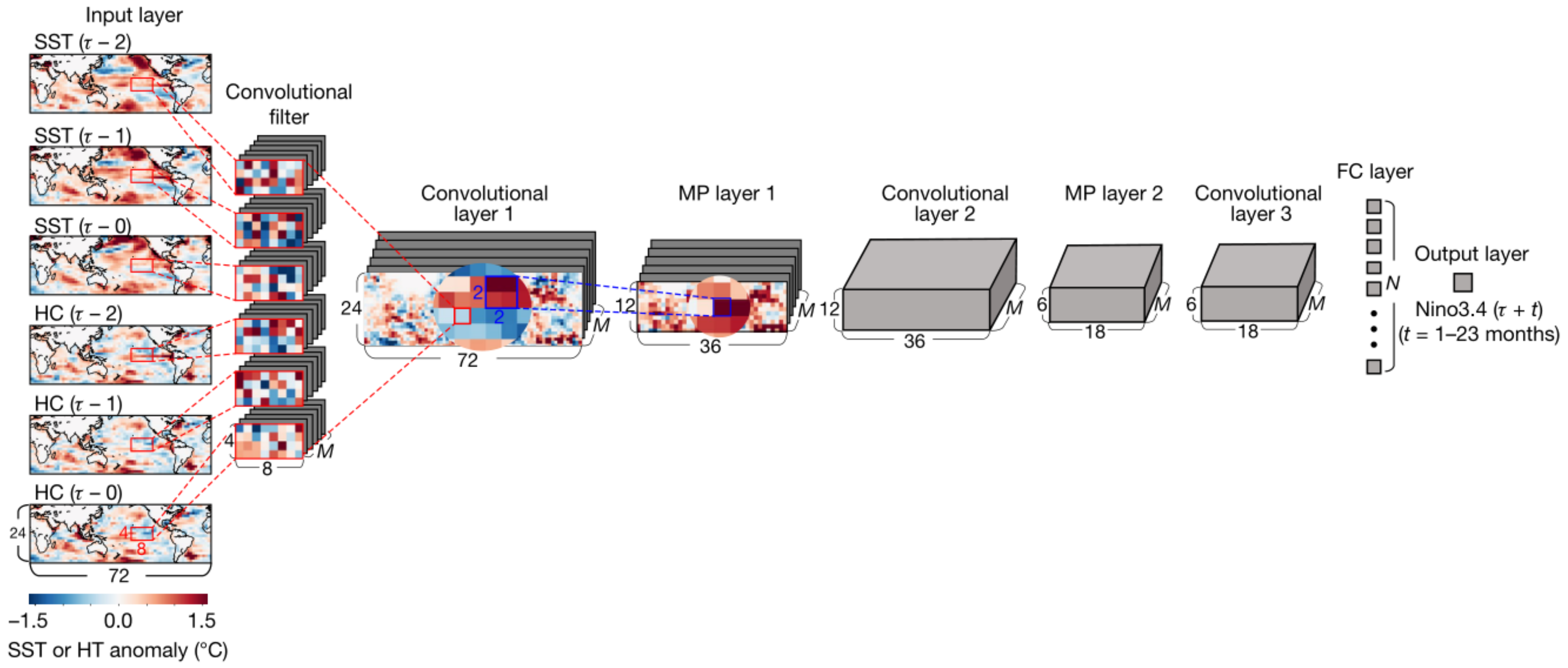
CNNs are applied in many fields of weather forecasting, and they are also helpful for ENSO forecasting. In September 2019, Ham et al. [51] first proposed using a CNN for ENSO prediction. The model structure is shown in Figure 3. CNN requires a large number of images for training in order to improve the accuracy of prediction. Despite the large scale of meteorological data, the use of CNNs in ENSO forecasting has encountered difficulties with data shortages. Ham et al. proposed to combine climate models with artificial intelligence methods, using dozens of global climate models from CMIP5 to generate a series of simulated data based on historical ocean data. As a result, scientists not only have a set of actual historical observations but also thousands of simulation results for training. The research results show that when the prediction time is more than 6 months, the prediction ability of the CNN method for the Nino3.4 index is significantly higher than that of the current international best dynamic prediction system. When tested on real data from 1984 to 2017, CNN was able to predict El Niño events 18 months in advance. At the time, the research results were regarded as the pioneering work of deep learning in the field of weather forecasting.

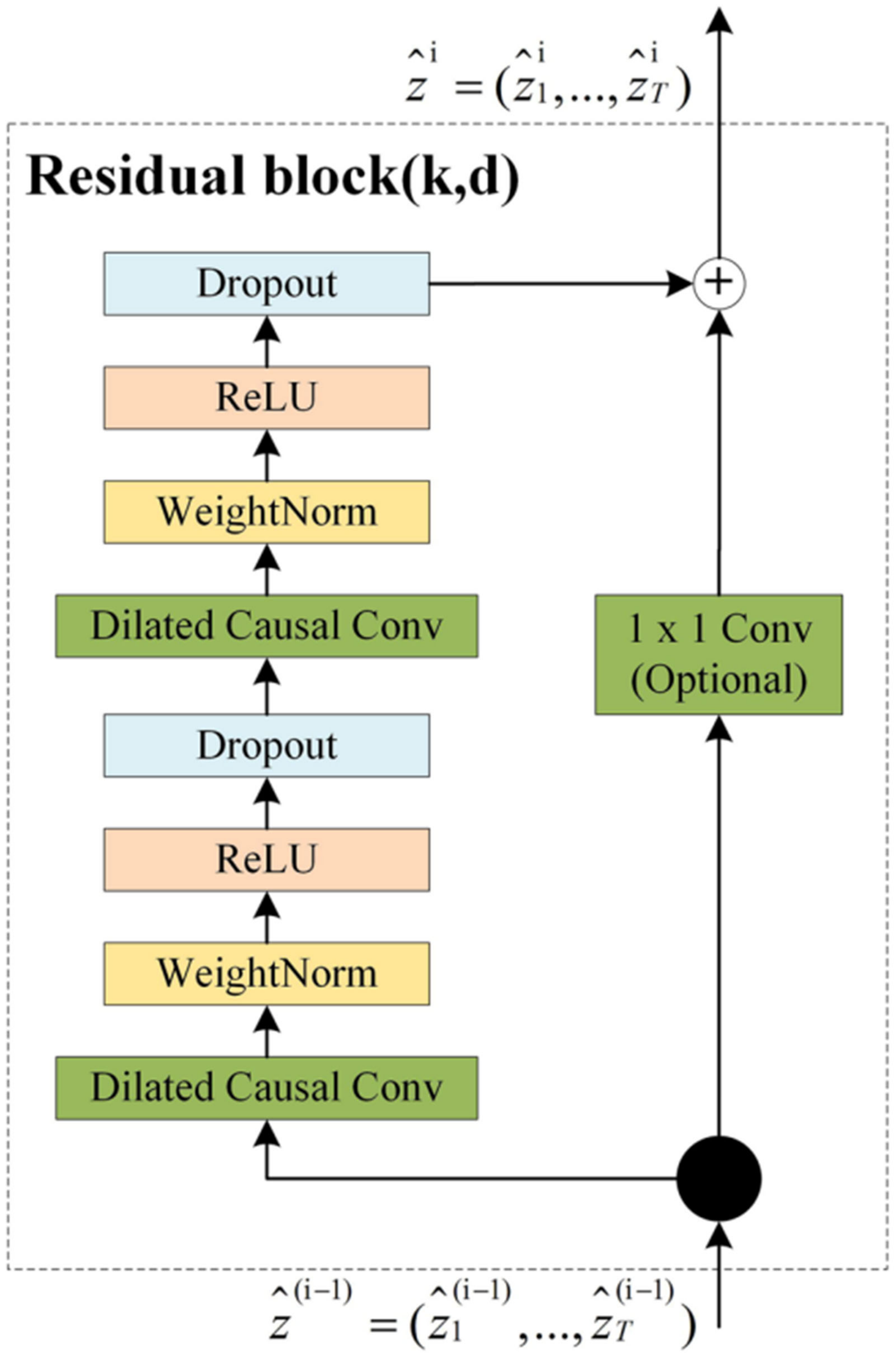
However, the defects of CNN itself, including fixed input vector size and inconsistent input and output size, limit its application in time-series forecasting. In 2020, Yan et al. [52] proposed the ensemble empirical mode decomposition-temporal convolutional network (EEMD-TCN) hybrid method, which decomposes the variable Niño3.4 exponent and SOI into relatively flat subcomponents; then, The TCN model is used to predict each subcomponent in advance, and finally, the sub-prediction results are combined to obtain the final ENSO prediction result. The TCN residual module diagram is shown in Figure 4. TCN is a variant of CNN that uses random convolution and dilation for sequential data with temporality and large receptive fields. Empirical mode decomposition can decompose high-frequency time series Niño 3.4 index and SOI data into multiple adaptive orthogonal components, improving the prediction accuracy of the model. The experimental results show that the TCN method has a good effect in the advance prediction of ENSO, which has important guiding significance for the research into ENSO. In response to the problem of data shortage, in addition to [51] using climate models to generate a large amount of simulated data, in 2021, Hu [53] et al. used dropout and transfer learning to overcome the problem of insufficient data during model training and proposed a model based on a deep residual convolutional neural network. The model effectively predicts the Niño 3.4 index with a lead time of 20 months during the 1984–2017 evaluation period, three months more than the existing optimal model. In addition, they also use heterogeneous transfer learning. This model achieved 83.3% accuracy for forecasting the 12-month-lead EI Niño type. However, many forecasts only consider temporality and the lack of spatial features in ENSO. 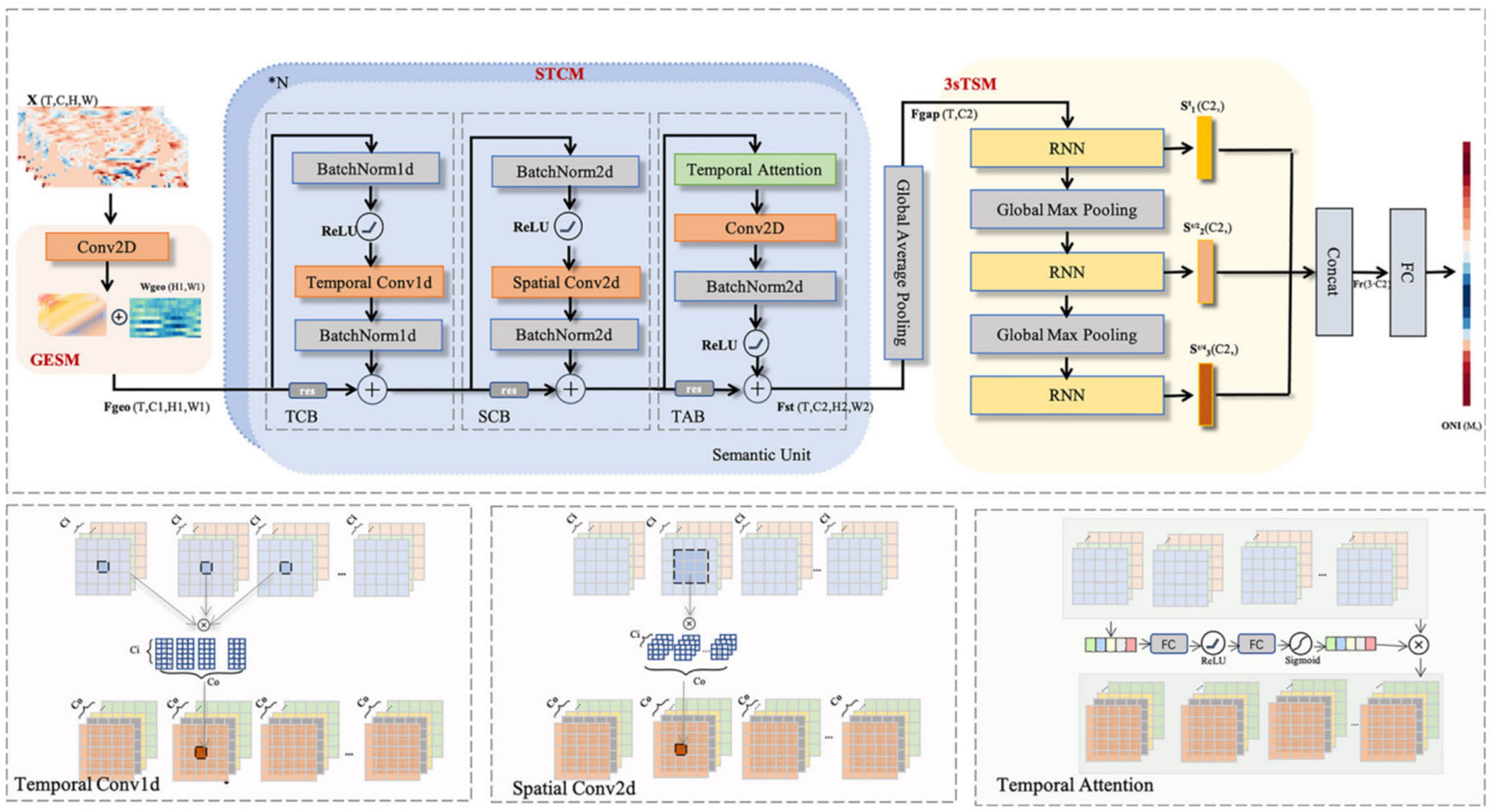In 2022, Zhao [54] et al. proposed an end-to-end spatial temporal semantic network, named STSNet, which consists of three main modules: (1) Geographic semantic enhancement module (GSEM) distinguishes various latitude and longitude through a learnable adaptive weight matrix; (2) A novel spatiotemporal convolutional module(STCM) is designed specially to extract the multidimensional features by alternating the execution of temporal and spatial convolution and temporal attention; (3) Combining and exploiting multi-scale temporal information in a three-stream temporal scale module (3sTSM) to further improve performance. Figure 5 illustrates the pipeline of the proposed STSNet. The results show that STSNet can simultaneously provide effective ENSO predictions for 16 months with higher correlation and lower bias compared to other deep learning models.

3.3. Recurrent Neural Network

When the input data has dependencies and is a sequential pattern, the results of CNNs are generally not very good, because there is no correlation between the previous input of the CNN and the next input. In 1982, Hopfield [55] proposed RNN. RNN is used to solve the problem that the training sample input is a continuous sequence, and the length of the sequence is different, such as the problem based on the time series. RNNs enable deep learning models to make breakthroughs in solving problems in NLP domains such as speech recognition [56], language models [57], machine translation [58], and time series analysis. In 1997, Jurgen Schmidhuber et al. 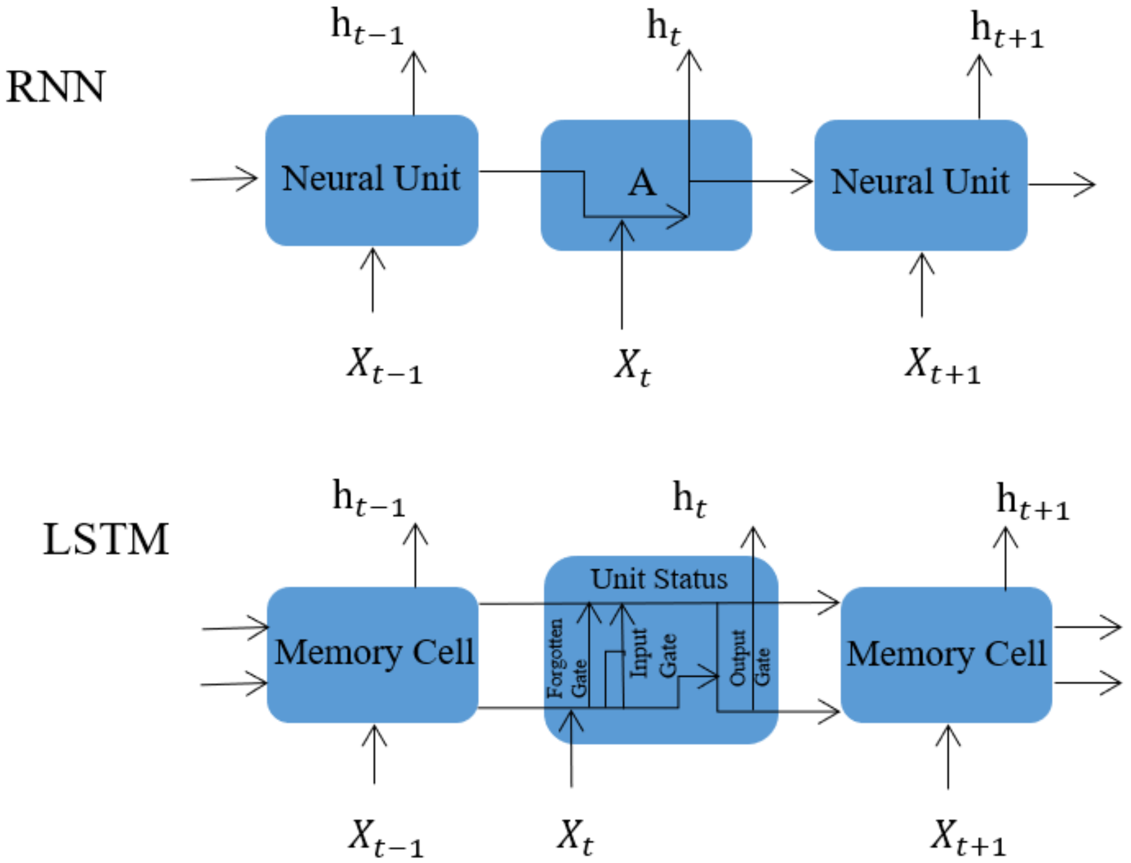[59] proposed long short-term memory (LSTM), a novel RNN variant structure that uses gating units and memory mechanisms to capture long-term temporal dependencies, and successfully solves gradient disappearance and the explosion problem, which controls the flow of information through learnable gates. The structure comparison of RNN and LSTM is shown in Figure 6. Among them, LSTM introduces the concepts of the forgetting gate, input gate, and output gate, thus, modifying the calculation method of the hidden state in RNN. The formula is as follows:

$$I_t=\sigma \left(X_t{W}_{xi}+H_{t-1}{W}_{hi}+b_i\right)$$

(16)

$$F_t=\sigma \left(X_t{W}_{xf}+H_{t-1}{W}_{hf}+b_f\right)$$

(17)

$$O_t=\sigma \left(X_t{W}_{xo}+H_{t-1}{W}_{ho}+b_o\right)$$

(18)

Among them, $W_{xi}$,$W_{xf}$,$W_{xo}$ and $W_{hi}, W_{hf}, W_{ho}$ are all learnable weight parameters, and $b_i, b_f, b_o$ are learnable offset parameters. The candidate cell in long short-term memory $\widetilde{C_t}$ uses the hyperbolic tangent function $\tanh$ in the range [−1, 1] as the activation function:

$$\widetilde{C_t}=\mathit{tanh}(X_t{W}_{xc}+H_{t-1}{W}_{hc}+b_c)$$

(19)

The flow of information in the hidden state can be controlled by input gates, forgetting gates, and output gates with element values in the range [0, 1]: this can usually be performed with the element-wise multiplication operator $\odot$. The calculation of the cell $\widetilde{C_t}$ at the current moment combines the information of the cell at the previous moment and the candidate cell at the current moment, and controls the flow of information through the forgetting gate and the input gate:

$$C_t=F_t\odot C_{t-1}+I_t\odot \widetilde{C_t}$$

(20)

Next, the information flow from the cell to the hidden layer variable $H_t$ can be controlled by the output gate:

$$H_t=O_t\odot \tanh \left(C_t\right)$$

(21)

In 2017, Zhang, Wang [60], and others defined the SST prediction problem as a time-series regression problem and used LSTM as the main layer of the network structure to predict the Bohai Sea temperature. The experimental results compared with SVR show that the LSTM network has better prediction performance. In 2018, Clifford et al. [61] used the “climate complex network” to extract meteorological data features, used the extracted features as predictors, and used LSTM to predict the Nino3.4 index. Experiments show that training LSTM models on network metric time series datasets has great potential for predicting ENSO phenomena many steps ahead. In 2021, Zhou et al. [62] used LSTM to build a tropical Pacific Niño3.4 index forecast model and analyzed the seasonal forecast error of the model. The results show that for the 1997/1998 and 2015/2016 strong eastern-type El Niño events, the model can more accurately predict the trends and peaks of the events, and the anomalous correlation coefficient (ACC) reaches more than 0.93. However, for the 1991/1992 and 2002/2003 weak central El Niño events, it did not perform well in peak forecasting.

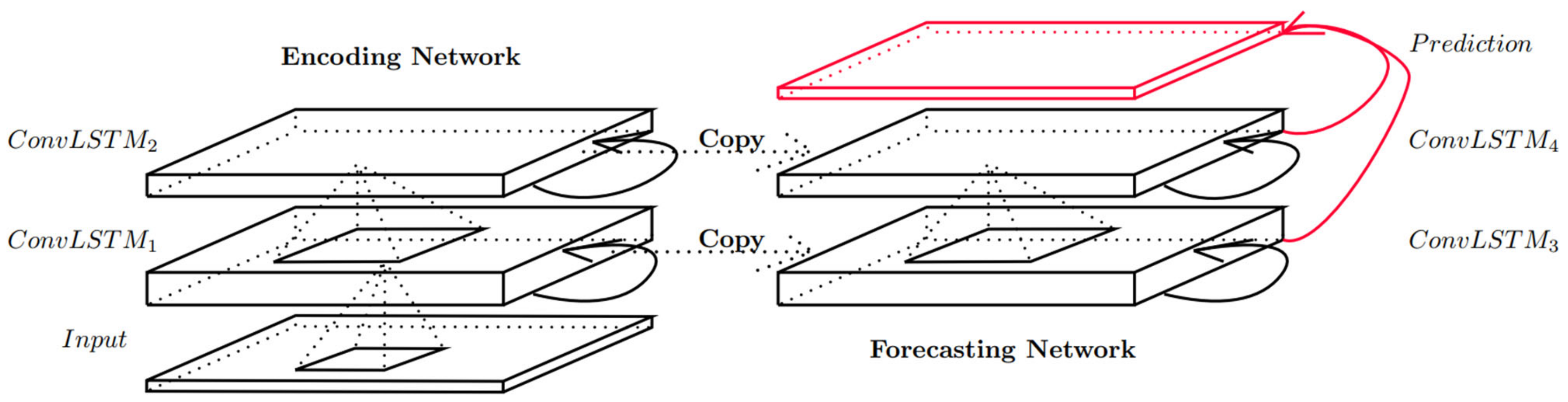
Shi X et al. [63] proposed the concept of convolutional long short-term memory (ConvLSTM) and established an end-to-end trainable for the precipitation now-prediction problem by stacking multiple ConvLSTM layers to form an encoder–decoder structure The model diagram is shown in Figure 7. ConvLSTM is designed to solve the problem of 3D data prediction; the unit can receive 2D matrices and even higher dimensional inputs at each time step. The key improvement is that the Hadamard product between the weights and the input is replaced by a convolution operation, as shown in Equation (22). It can not only establish temporal relationships similar to LSTM but also describe local spatial features by extracting features similar to CNN.

$$i_t=\sigma \left(W_{xi}\ast X_t+W_{hi}\ast X_{t-1}+b_i\right)$$

$$f_t=\sigma \left(W_{xf}\ast X_t+W_{hf}\ast H_{t-1}+b_f\right)$$

$$o_t=\sigma \left(W_{xo}\ast X_t+W_{ho}\ast H_{t-1}+b_o\right)$$

(22)

$$\widetilde{C_t}=\tanh \left(W_{xc}\ast X_t+W_{hc}\ast H_{t-1}+b_c\right)$$

$$C_t=f_t\odot C_{t-1}+i_t\odot \widetilde{C_t}$$

$$H_t=o_t\odot \tanh \left(C_t\right)$$

Among them, “$\ast$” represents the convolution operation, “$\odot$” represents Hadamard product. The difference between ConvLSTM and LSTM is only that the input-to-state and state-to-state parts are replaced by fully connected calculations with convolution calculations.

In 2019, Dandan He et al. [64] established a deep learning ENSO prediction model (DLENSO) using ConvLSTM to predict ENSO by directly predicting SST in the tropical Pacific. DLENSO is a sequence-to-sequence model. Its encoder and decoder are both ConvLSTM, and the input and prediction targets are both spatiotemporal sequences. DLENSO is superior to the LSTM model and the deterministic prediction model and is almost equivalent to the ensemble average in the medium and long-term prediction models. 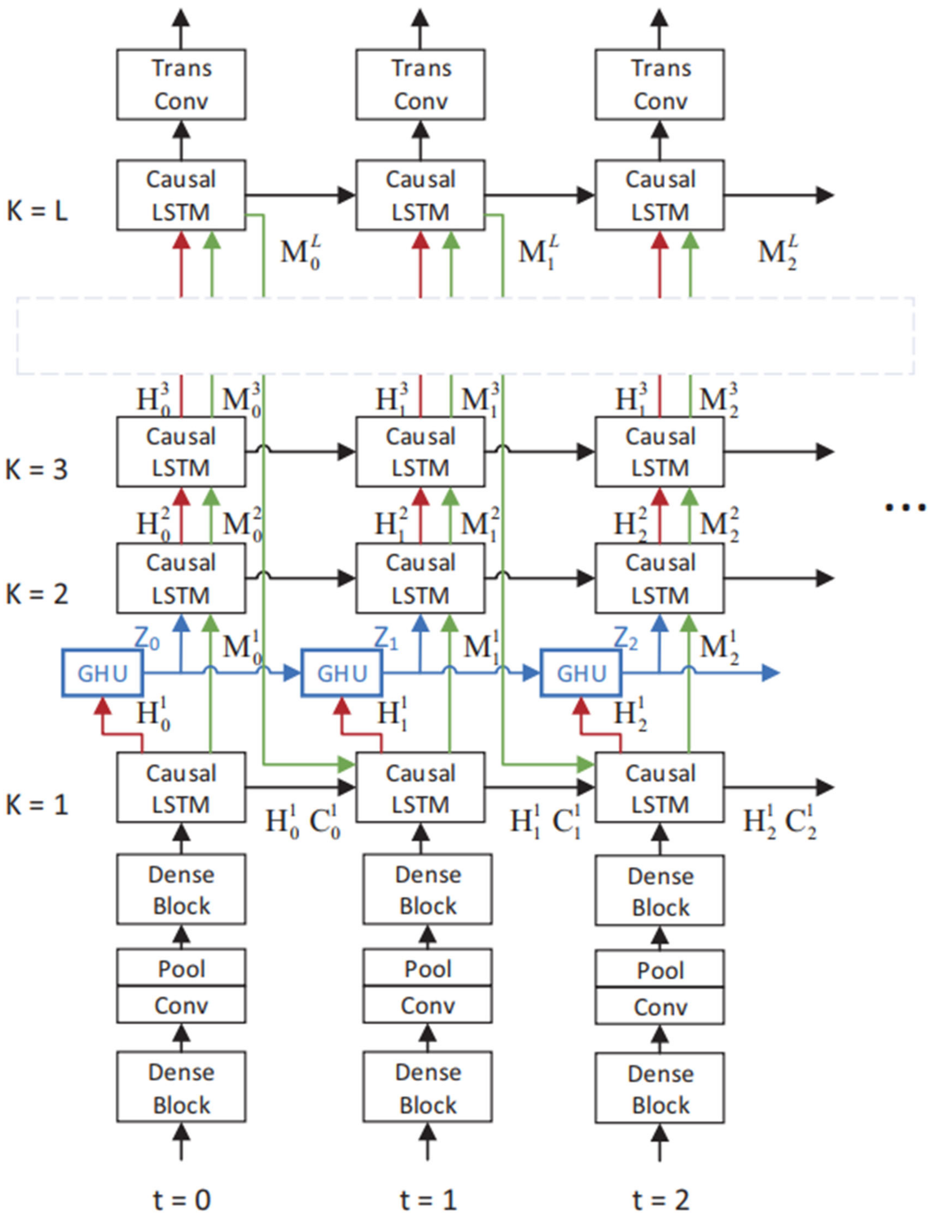To capture both spatial and temporal correlations in SST and improve prediction skills over longer time horizons, Mu [65] et al. proposed the ConvLSTM-RM model, which is a hybrid of convolutional LSTM and rolling mechanism, and used it to build an end-to-end trainable model for the ENSO prediction problem. Their experiments on historical SST datasets show that ConvLSTM-RM outperforms seven well-known methods on multiple time horizons (6 months, 9 months, and 12 months). The deep learning methods used above are all supervised learning, the training data are all labeled, and the cost of data labeling is often huge. In recent years, unsupervised learning has been mined and gradually developed. The biggest advantage of unsupervised learning is that it does not need to label the data so it can save a lot of manpower and resources. At the same time, compared with the limited labels marked by supervised learning, the features that can be learned by unsupervised learning are more adaptive and rich. In 2021, Geng et al. [66] regarded ENSO prediction as an unsupervised spatiotemporal prediction problem and designed a dense convolution–long short-term memory (DC-LSTM). The model diagram is shown in Figure 8. To obtain a more adequately trained model, they added historical simulated data to the training set. The experimental results show that the DC-LSTM method is more suitable for large area and single factor prediction. During the 1994–2010 validation period, the full-season correlation ability of the Nino3.4 index of DC-LSTM was higher than that of the existing dynamic models and regression neural networks, and the prediction effect for a lead time of up to 20 months was much higher than [51]. In 2022, Lu et al. [67] developed a new hybrid model, POP-Net, to predict SST in Niño 3.4 regions by combining POP analysis procedures with CNN and LSTM. POP-Net achieved a high correlation of 17-month lead-time predictions (correlation coefficient over 0.5) during the 1994–2020 validation period. In addition, POP-Net also mitigates SPB.

RNNs also have their own flaws. The RNN is often used to process sequence data, but the disadvantage is that it is not suitable for long sequences, and the gradient is easy to vanish. LSTM is proposed to deal with the problem of gradient disappearance. It is especially suitable for long sequences, but the disadvantage is the large amount of calculation; GRU is proposed to simplify the calculation of LSTM; obviously, GRU lost a gate in LSTM. Obviously, if the parameters are less, the natural calculation will be faster. When the training set is large, the performance is naturally not as good as LSTM.

3.4. Graph Neural Networks

The concept of GNN was first proposed by Gori [68] and others in 2005. The RNN framework was used to deal with undirected graphs, directed graphs, labeled graphs, and cyclic graphs. The feature map and node aggregation of the method generate a vector representation for each node, which cannot well deal with the complex and changeable graph data in reality. Bruna et al. [69] proposed to apply CNN to graphs, and through clever transformation of convolution operators, they proposed the graph convolutional network (GCN) and derived many variants. The proposal of GCN is the “pioneering work” of the graph neural network. For the first time, the convolution operation in image processing is simply used in the processing of graph structure data, which reduces the computational complexity of the graph neural network model. The calculation of the Laplacian matrix in the calculation process has since become past tense. Supposing we have a batch of graph data, which has N nodes and each node has its own characteristics, we let the characteristics of these nodes form an N × D-dimensional matrix X, and then the relationship between each node will also form an N × D. An N-dimensional matrix A is called an adjacency matrix. X and A are the inputs to our model, and the formula for GCN is as follows:

$$H^{\left(l+1\right)}=\sigma \left({\tilde{D}}^{-\frac{1}{2}}\tilde{A}{\tilde{D}}^{-\frac{1}{2}}{H}^{\left(l\right)}{W}^{\left(l\right)}\right)$$

(23)

Among them, $\tilde{A}=A+I$, $I$ is the identity matrix; $\tilde{D}$ is the degree matrix of $\tilde{A}$; H is the feature of each layer; for the input layer, H is X; $\sigma$ is the nonlinear activation function. The model of GCN is shown in Figure 9.

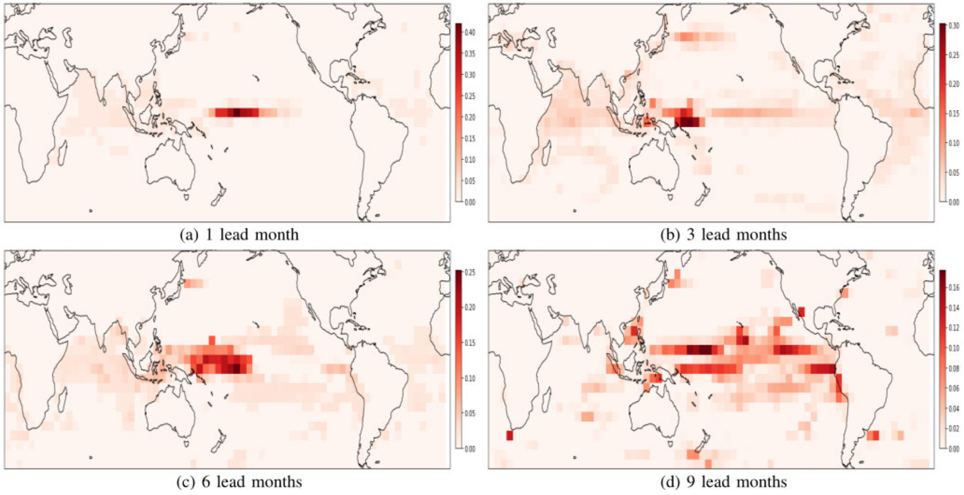
In 2021, Cachay et al. [70] first proposed the application of a graph neural network in seasonal forecasting and published it in NIPS. They advocated defining the ONI prediction problem as a graph regression problem and modeled it using GNNs that generalized convolutions to non-Euclidean data, thus, allowing us to model large-scale global connections as edges of the graph, except in graph convolutional neural networks, and they also designed a new graph-connected learning module to enable GNN models to learn large-scale spatial interactions together with practical ENSO prediction tasks. The model surpasses the state-of-the-art deep learning-based CNN model in ENSO prediction, and is also more effective than the LSTM model and the dynamic model, and its correlation coefficients in ENSO predictions 1 month, 3 months, and 6 months ahead of time reach 0.97, 0.92, and 0.78. 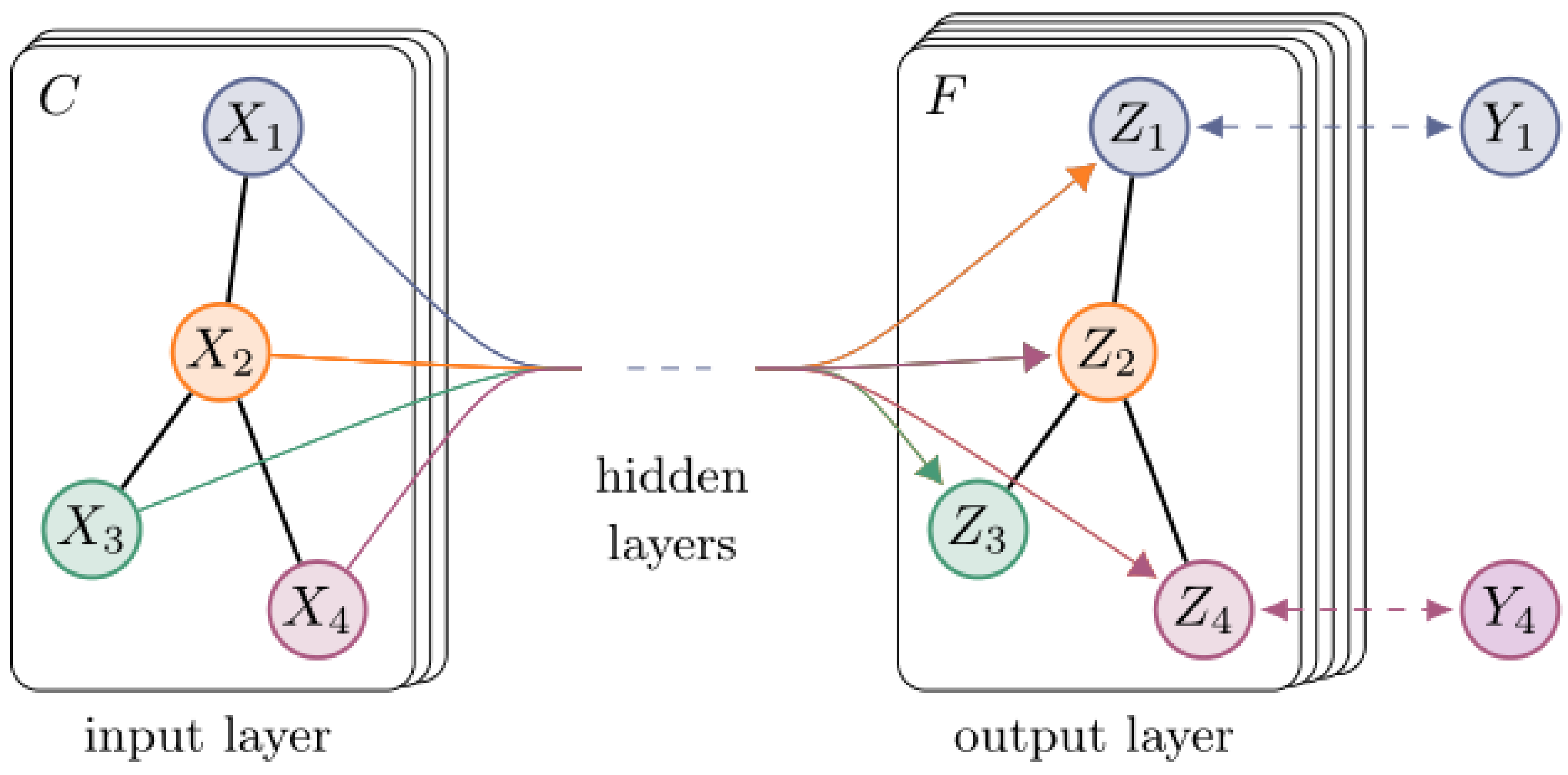The heat map of its effect is shown in Figure 10. Simply using the graphical model can achieve such excellent results. If the graphical model is combined with the power coupler, will there be new gains? Practice brings true knowledge. 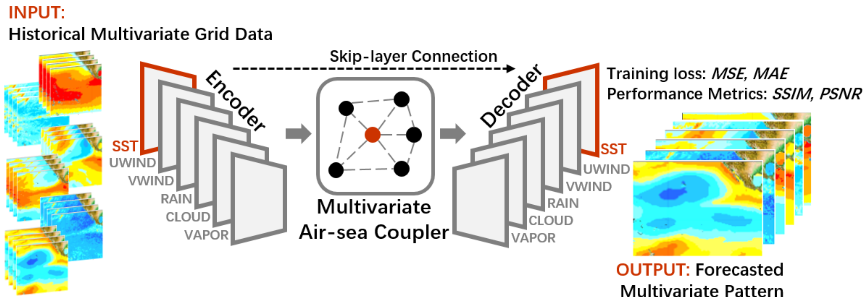Bin [71] et al. designed a graph-based multivariate air–sea coupler (ASC) using the features of multiple physical variables to learn multivariate synergy through graph convolution. Based on this coupler, an ENSO deep learning prediction model, ENSO-ASC, was proposed, which uses stacked ConvLSTM layers as the skeleton of the encoder to extract spatiotemporal features, and the decoder consists of stacked transform convolutional layers and upsampling layers. The model structure diagram is shown in Figure 11. The experimental results show that ENSO-ASC outperforms other models; sea surface temperature and zonal wind are two important predictors; and the Niño 3.4 index has correlations of over 0.78, 0.65, and 0.5 for lead times of 6, 12, and 18 months, respectively. Through this case, we can see that combining deep learning models with multivariate air–sea couplers or other dynamical models can improve the effectiveness and superiority of predicting ENSO and analyzing underlying dynamical mechanisms in a complex manner.

However, many recent cross-domain studies have found that GNN models do not provide the expected performance. When the researchers compared them to simpler tree-based baseline models, GNNs could not even outperform the baseline models. GNN can only perform feature denoising and cannot learn nonlinear manifolds. GNNs can, therefore, be viewed as a mechanism for graph learning models (e.g., for feature denoising) rather than as a complete end-to-end model. It has to be said that GNN, as an emerging neural network, has great prospects for development.

4. Discussion

We summarize the traditional and deep learning methods for ENSO prediction listed in this paper in

Table 1. Summary of deep learning and its application in ENSO forecasting.

Method	Specific Method		Generalize	Features
Traditional Method	Dynamic Methods		Using dynamic equations, the ocean, atmosphere, land, and other spheres and their interactions are modeled, and the computer is gradually integrated to simulate the evolution of the atmosphere. Ranging from relatively simple physical models to comprehensive fully coupled models.	The averaging skills of dynamic models are generally better than statistical models, but in practice, it is difficult to simulate the interannual average variation of sea surface temperature due to uncertainty in initial conditions. The emergence of SPB phenomenon.
	Statistical Methods	Linear Statistical Methods	Realize the analysis and prediction of ENSO phenomenon by sorting, summarizing, and analyzing historical ENSO indicators.	Statistical models require past long-term forecast data to discover potential relationships, but observations of the tropical Pacific did not begin until the 1990s. Compared to complex dynamic models, statistical models reduce cost and are easier to develop.
		Machine Learning Methods	Nonlinear statistical method, by learning and mining historical ENSO index features, using machine learning models to capture the nonlinear features of ENSO for prediction.
Deep Learning Methods	Convolutional Neural Network		CNN is a kind of feed-forward neural network with convolution calculation and deep structure from inputting original information, self-learning features, as the network goes from front to back, combining features from shallow to deep.	The forecasting skills of CNN are much higher than the current state-of-the-art dynamic models and can also better predict the detailed regional distribution of SST, overcoming the weaknesses of the dynamic prediction models. CNN is less affected by SPB, but it is not suitable for time-series forecasting.
	Recurrent Neural Network		RNNs are a pattern for text, sequence data recognition. Its input includes more than just the currently seen input example. It also includes information that the network perceives at the last minute. Using this property, information can circulate in the network for any length of time. Including LSTM, ConvLSTM, ConvGRU, etc.	RNN is suitable for solving sequence problems with continuous and different length of training sample input, such as time-series-based problems. The model can more accurately predict the trend and peak of strong El Niño events, but it is not good for weak El Niño peaks.
	Graph Neural Network		GNN is a deep learning method based on a graph structure, where data is represented in the form of a graph, and information flow is explicitly modeled through edge connections.	The gridded climate data can be naturally mapped to the nodes of GNN, and the prediction effect of GNN in the first 6 months exceeds the current state-of-the-art CNN model. However, there are still problems such as difficulty in predicting extreme ENSO events and limited training samples.

. More than half a century of ENSO research has achieved significant results, especially the possibility of real-time prediction of its advance month–season scale, such as the current linear statistical models or the dynamic models based on mathematical equations can predict ENSO at least 6 months in advance. We have achieved better real-time forecasting, but there are still large errors and uncertainties in forecasting skills. On the other hand, deep learning methods were put into use in ENSO forecasting and have greatly improved our forecasting ability for ENSO. The experimental indicators show that most spatiotemporal neural networks are suitable for ENSO prediction. Although deep learning methods can improve the accuracy of ENSO forecasting, artificial intelligence methods are not developed for the field of science, and research using neural networks to predict climate phenomena is still in its infancy, so there are still many problems.

First, deep learning has better modeling capabilities on the basis of big data, while the number of climate observation samples is small, especially for extreme events. In this case, the self-learning ability of deep learning methods is greatly limited, so the development of deep learning methods for small sample events is a current development direction. Second, in recent years, deep learning models have become more and more complex. Generally speaking, the more complex the model, the better its learning ability, but the problem is that the interpretability of the model results is worse.

In addition, when making long-term predictions, the prediction of ENSO event peaks has the problem of underestimation and prediction lag. We could try to introduce some random disturbance mechanisms so that the model can predict greater intensity. ENSO will also have the SPB problem in long-term forecasting, which is a difficult point in dynamic forecasting. More in-depth parameter adjustment work can be performed on the learning rates of different optimizers in the deep learning model, perhaps by finding hyperparameters that mitigate SPB in the training set. In addition, in order to improve the accuracy and length of ENSO predictions, we could try the spatiotemporal prediction model and graph neural network model recently proposed by AI, and use observation data and simulated data for training to increase the amount of training data. With sufficient data, we may be able to train a better model. At present, most of the research on artificial intelligence to improve ENSO prediction and other aspects mainly stays on the direct application of related artificial intelligence technology. Considering that phenomena such as ENSO in earth science research have clear temporal and spatial structures and evolution laws of physical processes, the ability to organically combine the temporal and spatial evolution characteristics of ENSO based on physical analysis methods with artificial intelligence methods based on big data to further improve ENSO Forecasting skills is a hot topic in the field of climate change. It is also worth continuing to explore how to combine deep learning with meteorology and climate in the future.

5. Conclusions

The severe cold and heat caused by the climate change caused by ENSO affect people’s daily life, and improving the accuracy of ENSO prediction is still a direction that researchers need to work on. This paper summarizes the main knowledge and development status of ENSO forecasting, including traditional ENSO forecasting methods and the application of artificial intelligence in ENSO forecasting. In this paper, artificial intelligence methods are divided into machine learning methods and deep learning methods. In the section on machine learning, the main methods such as decision tree, Bayesian, support vector machine and ARIMA are reviewed in ENSO forecasting. In the deep learning section, we summarized convolutional neural networks, recurrent neural networks, graph neural networks and their variants, focusing on the performance of these models in ENSO prediction. Table 1 provides an overview of various ENSO prediction methods and compares the advantages and disadvantages of each method. From the introductions in Section 2 and Section 3, it can be seen that the application of deep learning in ENSO prediction is widely effective and has great potential to further improve the prediction accuracy and length. By combining deep learning and meteorological science, researchers have drawn more conclusions, contributing to better climate predictions in the future. Finally, we analyzed the problems and research directions of artificial intelligence in ENSO prediction for future researchers’ reference and further development and better use of deep learning to expand more ways to help predict ENSO and even other climate problems.