Abstract
In the team orienteering problem, a fixed fleet of vehicles departs from an origin depot towards a destination, and each vehicle has to visit nodes along its route in order to collect rewards. Typically, the maximum distance that each vehicle can cover is limited. Alternatively, there is a threshold for the maximum time a vehicle can employ before reaching its destination. Due to this driving range constraint, not all potential nodes offering rewards can be visited. Hence, the typical goal is to maximize the total reward collected without exceeding the vehicle’s capacity. The TOP can be used to model operations related to fleets of unmanned aerial vehicles, road electric vehicles with limited driving range, or ride-sharing operations in which the vehicle has to reach its destination on or before a certain deadline. However, in some realistic scenarios, travel times are better modeled as random variables, which introduce additional challenges into the problem. This paper analyzes a stochastic version of the team orienteering problem in which random delays are considered. Being a stochastic environment, we are interested in generating solutions with a high expected reward that, at the same time, are highly reliable (i.e., offer a high probability of not suffering any route delay larger than a user-defined threshold). In order to tackle this stochastic optimization problem, which contains a probabilistic constraint on the random delays, we propose an extended simheuristic algorithm that also employs concepts from reliability analysis.
MSC:
68T20; 90-08; 90-10; 90Bxx; 90B06; 62Nxx
1. Introduction
The team orienteering problem (TOP) has been used to model operational challenges related to unmanned aerial vehicles (UAVs) [] as well as road electric vehicles and ride-sharing mobility actions in smart cities []. In this paper, we tackle the team orienteering problem with probabilistic delays (TOP-PD). As illustrated in Figure 1, we consider the realistic situation in which travel times between any pair of nodes i and j () in a set V might be subject to uncertainty due to the existence of a random delay . Using historical data, it will be assumed that we have been able to model each by a best-fit probability distribution. Thus, is composed of the minimum time required to travel from node i to node j () under ideal circumstances (e.g., no traffic jams, excellent weather conditions, etc.) which will be positive and a . In our TOP-PD, a fixed fleet of vehicles departs from a common origin location and has to reach a common finish location on or before a given deadline d strictly greater than the maximum of the expected values of , . Vehicles can visit some of the available nodes in V along their trip, thus collecting the corresponding reward. Thus, a reward is obtained the first time node is visited by any vehicle (notice that re-visiting a node does not provides any further reward; hence, it only makes sense to include a node in at most one route). Therefore, our main goal is to maximize the total reward collected by the fleet. However, while designing our routing plans, we will also need to guarantee a certain reliability level, i.e., the proposed solution is required to have a low probability of suffering delays under a user-specified threshold, p. This probabilistic constraint, which might appear in many real-life applications, introduces noticeable challenges in the optimization problem.
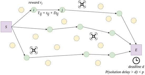
Figure 1.
A team orienteering problem with probabilistic delays.
As an effective way to solve such a challenging optimization problem, we propose the hybridization of a simheuristic algorithm [] and concepts from reliability analysis [,]. Using this extension of the simheuristic concept, we can generate the survival function associated with each TOP-PD solution. This function shows the probability that the routing plan experiences a delay of any size.
When using historical observations about delays in travel times, censored data might appear. Thus, for instance, we might know that a certain trip between two nodes suffered a delay between 5 and 10 min, but the exact value of that delay might not have been recorded. In the presence of such censored data, it is usual to employ the Kaplan–Meier method to obtain the survival function. Specifically, Kaplan–Meier is a non-parametric statistic used to estimate the survival function of censored time-to-event data [].
The main contributions of this paper are summarized next: (i) It proposes a new stochastic version of the TOP in which a probabilistic constraint linked to the delay times is included in the model; and (ii) it proposes a solving approach that combines a simheuristic algorithm with reliability concepts so that probabilistic information on delays can be considered even in the presence of censored data. The remaining sections of the paper are structured as follows: Section 2 briefly reviews related articles on the TOP as well as on simheuristic algorithms in routing problems. Section 3 provides a formal model of the considered problem. Section 4 describes the proposed simheuristic algorithm and its structure. Section 5 carries out a series of computational experiments to illustrate the performance of the proposed algorithm, while Section 6 analyzes the obtained results. Finally, the main findings and future research lines are given in Section 7.
2. Related Work
This section briefly reviews the existing literature on the team orienteering problem and also on the use of simheuristics to solve routing problems.
2.1. The Team Orienteering Problem
The Team Orienteering Problem is a variant of the well-known Vehicle Routing Problem (VRP). The main difference between the TOP and the VRP is that in the latter, a fleet of vehicles has to service all the customers trying to minimize the total cost, while the TOP aims to maximize the reward from a team of vehicles visiting a selection of nodes where there is a constraint on either the distance each vehicle can travel or the time that they are traveling [,]. It is likely that not all the customers can be visited; thus, the proper selection of the customers to be included in each vehicle’s route, as well as the order in which they have to be visited, constitute a challenge for the decision maker. Golden et al. [] introduced the Orienteering Problem, and Chao et al. [] proposed the classical version of TOP, a multi-vehicle extension of the original problem. These problems are NP-hard, and the the literature shows that deterministic versions of the TOP are chosen by many researchers, employing both exact [] or approximate [] methods. On the other hand, stochastic versions have not gained as much coverage to date mostly because of the increased difficulty entailed.
The following are some of the papers that focus on the exact methods for solving deterministic TOPs: Branch-and-Cut [,], Branch-and-Price [,,,], Branch-And-Cut-And-Price [], Cutting Planes [], and Column Generation [], In the last case, optimal solutions were also for mid-sized problems with up to 100 vertices. The main problem with exact methods is that the size of the TOP instances it can solve is usually reduced to a few hundred nodes, so many proposed metaheuristics can cope with large instances and reduce computational times to find near optimal solutions for the TOP problem. It includes Tabu Search [,], Variable Neighborhood Search algorithms [], Greedy randomized adaptive search procedure with path re-linking [], Ant Colony [], Particle Swarm Optimization [], Lion Optimization Algorithm [], Simulated Annealing [], Memetic Algorithm [], Pareto Mimic Algorithm [], Guided Local Search [], Hybrid Harmony Search [], or Genetic Algorithms [,]. These approaches improve the results obtained by the former heuristics, but the computational time to obtain a near-optimal solution also increases.
Although the stochastic TOP is more realistic than its deterministic alternative, it has been minimally studied in recent years. The case of a TOP with stochastic travel times is discussed in Panadero et al. [], and they also suggest a simheuristic algorithm, which combines a Variable Neighbourhood Search (VNS) metaheuristic with a Monte Carlo simulation to handle stochastic TOP efficiently. Similarly, a genetic programming hyperheuristic to solve a stochastic TOP with time windows is proposed in Mei and Zhang [], where the service times at each node are then modeled as random variables. A subscription delivery problem as a stochastic TOP with time windows and consistency in the driver assigned to each customer is analyzed in Song et al. []. Some studies also refer to the Orientation Problem (OP) with stochastic approximations, given it is a simplified version of the TOP but considering only one path. In this direction, Bian and Liu [] discuss the stochastic orientation problem at the operational level, where travel and service times are stochastic. The routing schedule can be refined in real time so that the collected reward and the probability of the vehicle arriving on time can be enhanced. Another extension of the OP with stochastic travel times is discussed in Dolinskaya et al. [], in which it is feasible to boost the probability of gathering a higher reward by adapting the routes between reward nodes as travel times are revealed. In addition, Dolinskaya et al. [] discuss an extension of the OP by considering stochastic travel times, increasing the probability of obtaining more reward as soon as travel times are known and then adapting the routes between reward nodes.
2.2. Using Simheuristics in Routing Problems
There is a lot of research conducted on the combination of simulation and metaheuristic optimization, also called simheuristics. Hence, for instance, Quintero-Araujo et al. [] apply simheuristics and a horizontal collaboration strategy to analyze the cost reduction of urban transportation modes under uncertainty. Two scenarios are defined: collaborative (modeled as one multi-depot VRP) and non-collaborative (modeled as a set of VRPs). As an example, garbage collection can be posed as a deterministic problem, and Gruler et al. [] studied how to provide a solution for collecting waste in smart cities. For this purpose, they developed a metaheuristic algorithm based on a variable neighborhood search framework. This problem could be extended to a stochastic version and use simheuristics to solve it, including a risk analysis taking into account the variance of the waste levels and the maximum capabilities of the vehicle.
VRP has variants, such as the two-dimensional vehicle routing problem (2L-VRP) and Guimarans et al. [] solved its stochastic version. For the case of electric vehicles, Reyes-Rubiano et al. [] solved the VRP problem. In this case, the constraints additionally included a limited driving range, and both the driving range of an electric vehicle and the travel time were considered stochastic. A fuzzy layer can also be considered, as in Tordecilla et al. [], so it combines simulation, metaheuristics, and fuzzy logic to handle the fuzzy uncertainty of travel times and customer demands. Other uncertainty in problem features could be characterized as a correlation between different elements of the problem. Stochastic and correlated customer demand in the VRP is analyzed in Latorre-Biel et al. [], and simheursitics are used to solve it. Optimization problems often use simulation, but it is an expensive tool. This is why simulation should be used only when necessary to reduce the overall computational time and still obtain promising solutions. Rabe et al. [] reviewed many ideas about the number of simulation runs and the need for them. Although their work focuses on a manufacturing system, analogous work is possible to have similar approaches in transportation and logistics.
3. Modeling the TOP with Probabilistic Delays
The TOP with probabilistic delays that was introduced before can be formalized as follows. Let us assume an undirected graph , where: (i) includes a set of n nodes, a starting node o, and an end node f; and (ii) E is the set of edges , with , connecting nodes and . There is a fixed fleet of vehicles initially located at o. In addition, there is a maximum time or deadline, , for completing each route (from o to f). The first time a node is visited, a reward is collected, while . Each edge has an associated travel time, , where is the minimum time required to traverse the edge in ideal travel conditions, and is a random variable representing a possible delay time. It is assumed that and also that and are the same random variable. Notice, however, that the proposed approach could still be employed even if these assumptions were not made (they simply allow us to reduce the size of the problem and are frequently employed in the related literature). A solution to the TOP is a set of routes departing from o, visiting a subset of nodes in a specified order and arriving at f. In order for a solution to be feasible, the probability that the maximum time employed by any route does not exceed the deadline d, plus a user-defined delay , has to be lower than a user-defined threshold , which represents an upper bound to the probability of suffering delays in a specific routing plan. Let us consider the binary decision variable , which takes the value 1 if the edge is used by a vehicle to collect the reward at node j, and 0 otherwise. In addition, let us define the random variable , which represents the total travel time that the vehicle has spent after visiting node j. We will assume that can be modeled according to a non-negative probability distribution, such as the Weibull, Gamma, or Log-Normal ones. Since uncertainty is present in most real-life processes and systems, considering random processing times represents a more realistic scenario than simply considering deterministic times. Then, the objective function is given by the maximization of the collected reward:
This objective function is subject to the following constraints:
If we denote as intermediate nodes those that differ from o and f, Constraints (2) and (3) impose that each intermediate node has at most one edge departing from it or entering it, respectively. In addition, Constraint (4) imposes that, for each intermediate node, the number of incoming edges is equal to the number of outgoing edges (due to the previous constraints, this value will be either 0 or 1). Constraint (5) ensures that the number of routes starting at the origin node is the same as the number of routes arriving at the sink node. Constraint (6) forces that the number of routes must be less than or equal to the number of available vehicles k. Two constraints, (7) and (8), are introduced for both the connectivity of the solution and the probabilistic constraint on the maximum delay allowed. Constraint (9) avoids degenerated routes with undesirable loops and connections. Finally, Constraints (10) and (11) define the range of the model variables.
4. An Extended Simheuristic with Reliability Concepts
To tackle the stochastic optimization problem described in the previous section, we propose a simheuristic algorithm. Our method combines biased-randomized techniques [] with simulation techniques to deal with the stochastic nature of the problem. The main characteristics of our approach are explained next.
4.1. A Biased-Randomized Algorithm for the Deterministic TOP
In order to address the deterministic version of the problem, we use a constructive heuristic that employs biased randomization techniques, allowing us to extend the deterministic heuristic into a probabilistic one while still preserving the logic behind the heuristic. Given the graph G previously described, the heuristic starts by generating an efficiency list of edges . Notice that each edge has two different arcs depending on the direction in which the edge is traversed. Afterwards, this list is sorted using an efficiency criterion, defined as a linear combination of the travel time required to traverse each edge and the aggregated reward generated by visiting the two extreme nodes, i and j. Algorithm 1 depicts the main procedure to compute the efficiency list. This function receives as parameters the set of nodes (including the origin and destination nodes) and a tuning parameter . This parameter is set for each instance, and its value will depend upon the heterogeneity level of the reward values in each particular instance. Thus, for instances with a high heterogeneity level, will tend to be chosen close to zero, while for instances with a low heterogeneity level, will be close to one. The function starts by assigning the starting and destination nodes. Next, the edges connecting node o with each node , as well as edges connecting each node i with the destination node f, are defined. At this point, the heuristic computes the ‘enriched savings’ value (efficiency criterion) for each pair of nodes , with , as follows. First, the cost of the edge is computed using the Euclidean distance. Then, the aggregated reward of the edge is computed as well. The formula to compute the efficiency value associated with an edge is expressed as , where represents the traveling time between i and j, and accounts for the aggregated reward. Finally, the efficiency list is sorted from higher to lower.
| Algorithm 1 Computing the efficiency list. | |
1: | input: |
2: | V: list of nodes without origin and end nodes |
3: | o: starting node |
4: | f: destination node |
5: | end input: |
6: | efficiencyList ← Ø |
7: | k ← getLength(V) |
8: | for
do |
9: | node ← getNode(n) |
10: | onEdge ← Edge(o, node) |
11: | nfEdge ← Edge(node, f) |
12: | onEdgeCost ← computeEuclideanDistance(o, node) |
13: | nfEdgeCost ← computeEuclideanDistance(node, f) |
14: | end for |
15: | for
do |
16: | iNode ← getNode(i) |
17: | for do |
18: | jNode ← getNode(j) |
19: | ijEdge ← Edge(iNode, jNode) |
20: | jiEdge ← Edge(jNode, iNode) |
21: | ijEdgeCost ← computeEuclideanDistance(iNode, jNode) |
22: | setCost(ijEdge, ijEdgeCost) |
23: | setCost(jiEdge, ijEdgeCost) |
24: | ijEfficiency ← computeEfficiency(iNode, jNode) |
25: | jiEfficiency ← computeEfficiency(jNode, iNode) |
26: | efficiencyList ← appendEdges(ijEdge, jiEdge) |
27: | sortEfficiencyList |
28: | end for |
29: | end for |
30: | return efficiencyList |
Once the efficiency list has been computed, the heuristic generates an initial ‘dummy’ solution, which assigns one ‘virtual’ vehicle per pick-up node, using as many of these virtual vehicles as the number of nodes in the problem. Specifically, in this ‘dummy’ solution, each virtual vehicle starts from the origin node o, visits a pick-up node, and then continues its trip towards the destination node f. Next, an iterative merging process starts: edges are selected from the sorted list, and the associated routes are merged as long as this merge does not violate any capacity or time constraint. Finally, the list of merged routes is decreasingly sorted according to the total reward. Routes with the highest rewards are selected, and the number of selected routes equals the number of available vehicles in the fleet. This constitutes an initial routing plan for the deterministic version of the problem.
The greedy heuristic described above can be extended into a probabilistic algorithm by using a skewed probability distribution during the edge-selection process. Hence, higher-efficiency edges are more likely to be ranked at the top of the list. This process lets edges be selected in a different order at each iteration of the process, while still preserving the flavor of the heuristic. In our case, a geometric probability is used to induce this skewed behavior. This allows us to quickly generate a huge number of good alternative solutions based on the efficiency criterion defined by the heuristic [].
4.2. A Simheuristic for the Stochastic TOP-PD
To solve the stochastic version of the problem, the biased-randomized heuristic described previously was extended into a complete simheuristic approach. Thus, the biased-randomized algorithm was integrated into a multi-start framework and combined with a Monte Carlo simulation (MCS) to efficiently estimate the expected time employed by each ‘promising’ solution proposed by the optimization component. First, a feasible initial solution was generated using the greedy version of the heuristic. Then, during a second stage, the muti-start schema tried to improve the initial solution by iteratively exploring the search space using the biased-randomized algorithm. The solutions generated using this methodology are deterministic and do not consider uncertainty. To deal with the stochastic nature of the problem, we include two simulation processes in different stages of our algorithm. In the first case, we conducted a short number of MCS runs to compute the expected travel time whenever the deterministic cost of the new generated solution improved the best-found solution so far. If the new solution also improved the stochastic cost of the best solution, the latter was updated and added to the pool of ‘elite’ solutions, i.e., those solutions that are among the best in stochastic cost. We limited the size of this pool to ensure that we only keep the elite solutions as the algorithm evolves.
This TOP-PD contains a probabilistic constraint, which allows the user to specify a delay parameter p, so that solutions have a probability smaller than p to experience a delay. If represents the total time invested by vehicle in completing its assigned route, then where and . For its implementation, a parameter will be introduced in the construction phase of the algorithm; represents an amount of time that will be subtracted from the allowed duration of any route. This ‘safety stock’ of time will help to satisfy the probabilistic constraint, i.e., that the probability of delay remains under p. Taking into account that our initial deadline is , if one of the routes in a solution takes longer than to finish, that extra time is the delay the solution is incurring. Altogether, the procedure goes as follows:
- The heuristic provides the deterministic solution for a . This is, we allow the routes to have maximum duration.
- If after a short simulation the probability of the solution incurring in a delay is greater than p, we will slightly increase . Therefore, the new deadline taken to construct the solutions will be , with and . Note that when a is found such that , it will be saved (), so the future solutions created by the algorithm will have deadline .
This procedure is represented in Figure 2. In conclusion, by limiting the routes’ maximum time, the probability of delay is reduced, since we force the algorithm to create routes with a tighter deadline , thus including less nodes and reducing the probability of having routes with a duration greater than . At the final phase of the simheuristic, only solutions with probability of delay smaller than p will be included in the elite pool of best solutions.
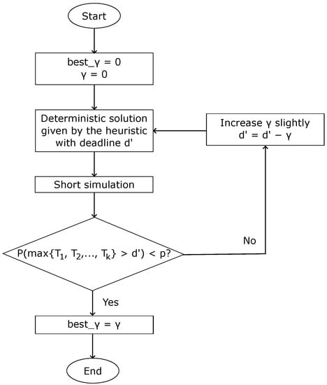
Figure 2.
flowchart.
Algorithm 2 provides an example of how a ‘promising’ solution could be evaluated under a stochastic scenario to compute the expected reward collected by the fleet of vehicles. First, the function initializes the auxiliary variables to compute the expected profit of the solution totalProfit. Then, the simulation runs are performed. Notice that the number of runs is an input parameter defined by the user. For each run, the function computes the time to complete each route of the solution, as well as its associated expected profit. Thus, the expected travel time is a summation of the deterministic travel time () to cross an edge and an estimated travel delay (), which is a random value according to the corresponding probability distribution. This result is accumulated into the route travel time. Notice that under stochastic travel times, the routes’ duration might be long enough to exceed the deadline, therefore incurring certain delay. Since we are interested in avoiding this behavior, every time a route exceeds the deadline we will force it to lose all of its profit. This way, the algorithm will prioritize solutions that are not that likely to experience delays, since after the simulation they will obtain a smaller reward and therefore be excluded. Back in Algorithm 2, the average reward is computed and stored. Rabe et al. [] offer a discussion on how more advanced simheuristic algorithms can be designed.
Once the first stage of the algorithm is finished, we carry out a large number of MCS runs to better assess the elite solutions of the pool before reporting the final results. Finally, the pool of solutions is sorted by the stochastic reward and the solution with the highest expected reward is returned. Since the number of generated solutions during the search can be large, and the simulation process is time-consuming, we limited the number of MCS runs in the first stage. In particular, we set up the number of runs for the exploratory and intensive MCS stages to 100 and 10,000, respectively.
| Algorithm 2 Simulating a solution. | |
1: | input: |
2: | numberSimulations: simulations runs |
3: | solutionRoutes: routes of the solution |
4: | deadline: upper time limit for all the routes |
5: | end input |
6: | stochasticProfit ← 0 |
7: | totalProfit ← 0 |
8: | k ← getLength(solutionRoutes) |
9: | for
do |
10: | simProfit ← 0 |
11: | for do |
12: | route ← getRoute(r) |
13: | routeEdges ← getEdges(route) |
14: | profit ← 0 |
15: | routeDuration ← 0 |
16: | n ← getLength(routeEdges) |
17: | for do |
18: | edge ← getEdge(routeEdges, e) |
19: | customer ← getEndNodeInEdge(edge) |
20: | customerProfit ← getCustomerProfit(customer) |
21: | if customerProfit > 0 then |
22: | ← getStochasticValue |
23: | edgeDuration ← getDuration(edge) |
24: | routeStochasticDuration ← edgeDuration + |
25: | routeDuration ← routeDuration + routeStochasticDuration |
26: | profit ← profit + customerProfit |
27: | end if |
28: | end for |
29: | if routeDuration > deadline then |
30: | profit ← 0 |
31: | end if |
32: | simProfit ← simProfit + profit |
33: | end for |
34: | totalProfit ← totalProfit + simProfit |
35: | end for |
36: | totalProfit ← totalProfit/numberSimulations |
37: | stochasticProfit ← totalProfit |
38: | return stochasticProfit |
5. Computational Experiments
The proposed simheuristic was implemented in Python and executed in a workstation with an Intel(R) Xeon(R) processor at GHz with 64 GB of RAM memory. To carry out the experiments, we adapted the well-known deterministic benchmarks proposed in Chao et al. []. These benchmark contain a total of 320 instances, which are divided in 7 different subsets. The instances are identified following the nomenclature ‘pa.b.c’, where ‘a’ represents the subset, ‘b’ defines the number of available vehicles, and ‘c’ identifies the specific instance under study. To adapt them to the stochastic context, we considered random travel times, , instead of the original deterministic travel times, . These random travel times increase the deterministic ones by adding a random delay associated with each edge, , i.e., . Due to their characteristics, the Weibull, Gamma, and Log-Normal probability distributions are frequently used to model positive processing times []. Still, among these, the Weibull distribution is usually preferred in reliability analyses due to its extraordinary flexibility []. For this reason, in our experiments we assumed that delays will follow a Weibull distribution with parameters and . In a real-life scenario, the specific probability distribution can be fitted from historical data, which allows for obtaining the best-fit probability distribution as well as its parameters.
Table 1 shows a summary of the computational results. We calculated the solutions under the constraint that the probability of delay cannot exceed . In practice, this means that the solution’s routes will finish on time with a probability of or higher. It can be seen that under a deterministic scenario with fixed travel times, the best deterministic solution always obtains the maximum reward (OBD column). However, when we simulate the best deterministic solution with stochastic travel times, the results change; it can be seen in column OBD-S that the reward decreases drastically. On the other hand, under a stochastic scenario, the best stochastic solution (OBS) outperforms the OBD-S. This effect can be clearly visualized in Figure 3.

Table 1.
Computational results.
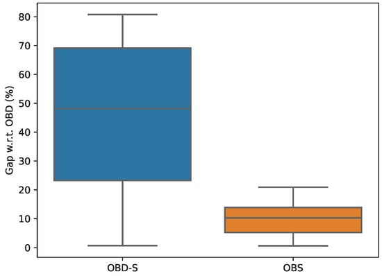
Figure 3.
Percentage gaps of OBD-S and OBS with regard to OBD.
6. Analysis of Results
The methodology we are presenting in this paper aims to offer decision makers three powerful mathematical possibilities when scheduling routes under uncertain travel times: (i) to define how much delay is acceptable taking into account the total reward collected; (ii) to choose a solution from the elite group of solutions; and (iii) to define a probabilistic constraint such that routes will not have a probability greater than a user-defined threshold p of incurring delays. Each of these dimensions will be discussed in the following subsections.
6.1. Impact of Delay Selection
In this first analysis, the impact of the ‘accepted’ delay will be addressed. The main idea is to show how increasing will produce a rise on the total reward collected. Through a graph that shows the trade-off between delay accepted and reward collected, the decision maker may decide to exchange the initial deadline d for a soft deadline in order to increase the reward.
Figure 4 shows the aforementioned trade-off graph for the instance p7.4.t. As we allow a higher delay, the routes will have more room to pick up additional passengers, therefore offering a bigger total reward. It can be seen that at , the total reward that the solution can provide reaches the maximum possible reward.
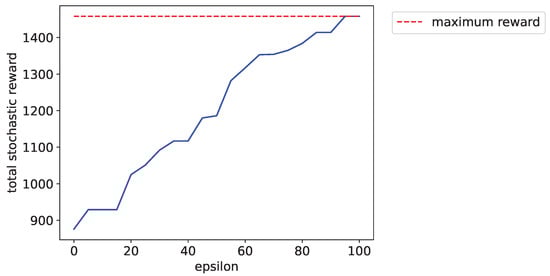
Figure 4.
Trade-off between accepted delay and total stochastic reward.
6.2. Probability of Incurring Different Delays
In order to choose a solution from the elite group of solutions, a survival function of each routing plan is obtained. To build this function, it was necessary to obtain the Kaplan-Meier estimator from the simulation outcome. The survival function offers the probability of incurring delays of different solutions or routing plans. In this way, we can compare different routing plans both in terms of the expected reward and the probability that they will finish for a certain target moment. For our analysis, we will focus on the top 3 solutions that our approach generated for instance p7.4.t. Figure 5 represents the Kaplan–Meier survival curves associated with each of the top 3 stochastic solutions obtained for the same expected reward. Note that clearly underperforms both and at any target time. On the other hand, outperforms until . At this point, both curves meet, having around survival probability (or probability that the routing plans can finish on or before the target time). After this moment, is the one whose curve falls faster, meaning that the probability of its routing plan being finished is smaller than the other two solutions.
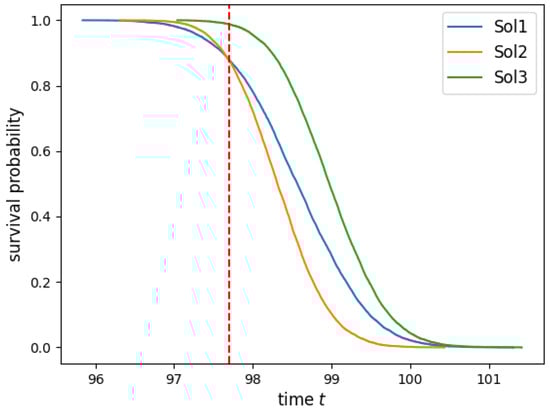
Figure 5.
Survival function for instance p7.4.t.
6.3. Reliability of a Solution
In this subsection, we will implement the probability constraint that will allow the solutions to have a low probability of suffering delays for a soft deadline , under a user-specified threshold p. If represents the total time invested by vehicle in completing its assigned route, then where and . For the sake of simplifying the experimentation process, we will consider . Nevertheless, the decision maker can choose any . Figure 6 shows the trade-off between gamma and the probability of delay for the instance p7.4.t with time units. When gamma increases, limiting the routes’ maximum duration, the probability of delay decreases, reaching a value close to 0 when we allow routes to have a maximum duration of 85 (). If, for example, the decision maker states that only solutions with a probability of delay under are allowed, then the algorithm will set , allowing routes to have a duration of only 90 time units.
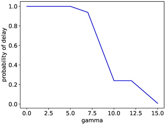
Figure 6.
Trade-off between gamma and probability of delay.
7. Conclusions and Future Work
In this paper, a stochastic version of the ride-sharing problem with random travel times is considered. Ride-sharing operations are modeled as a team orienteering problem. Here, drivers have to select which customers should be picked up in order to maximize the expected reward collected. At the same time, drivers should be able to reach their destination on or before a pre-established deadline. Of course, the existence of random travel times might be the source of delays in some routing plans. Depending on their size, these delays might be associated with a penalty cost that jeopardizes the benefits of the driver.
In order to provide high-quality solutions to this challenging stochastic optimization problem, we combine a simheuristic algorithm with concepts from survival analysis. Thus, our optimization-simulation approach is not just able to generate ‘elite’ solutions with high expected rewards, but it also offers probabilistic information about the size of the delays associated with each of these elite solutions. This information might be valuable for managers since they have a more complete understanding of the probabilistic behavior or each proposed routing plan. Hence, questions such as “what is the probability that a specific routing plan causes some of our customers to be late by more than 10 min” can be properly answered.
Regarding future work, we plan to carry out the following extensions: (i) to consider a scenario in which correlations among delays might occur—e.g., when a geographical area becomes congested, all paths in the area will be subject to high delays; (ii) to extend the simheuristic approach by including a machine learning component that makes use of the simulation feedback to better guide the metaheuristic search in the space of solutions; (iii) apply a parametric Weibull model to fit a survival function and compare its fit with the non-parametric Kaplan–Meier model; and (iv) to predict with the best-fit survival model.
Author Contributions
Conceptualization, A.A.J. and J.P.; methodology, A.A.J. and P.C.; software, E.M.H. and J.P.; writing—original draft preparation, A.A.J., E.M.H., E.P.-B., P.C. and J.P.; writing—review and editing, A.A.J., E.P.-B. All authors have read and agreed to the published version of the manuscript.
Funding
This work has been partially funded by the Spanish Ministry of Science (PID2019-111100RB-C21-C22/AEI/10.13039/501100011033), the Barcelona City Council and Fundació “la Caixa” under the framework of the Barcelona Science Plan 2020–2023 (grant 21S09355-001), and the Generalitat Valenciana (PROMETEO/2021/065).
Institutional Review Board Statement
Not applicable.
Informed Consent Statement
Not applicable.
Data Availability Statement
Not applicable.
Conflicts of Interest
The authors declare no conflict of interest.
References
- Bayliss, C.; Juan, A.A.; Currie, C.S.; Panadero, J. A learnheuristic approach for the team orienteering problem with aerial drone motion constraints. Appl. Soft Comput. 2020, 92, 106280. [Google Scholar] [CrossRef]
- Panadero, J.; Ammouriova, M.; Juan, A.A.; Agustin, A.; Nogal, M.; Serrat, C. Combining parallel computing and biased randomization for solving the team orienteering problem in real-time. Appl. Sci. 2021, 11, 12092. [Google Scholar] [CrossRef]
- Chica, M.; Juan, A.A.; Bayliss, C.; Cordón, O.; Kelton, W.D. Why Simheuristics? Benefits, Limitations, and Best Practices when Combining Metaheuristics with Simulation. Stat. Oper. Res. Trans. 2020, 44, 311–334. [Google Scholar] [CrossRef]
- Emmert-Streib, F.; Dehmer, M. Introduction to survival analysis in practice. Mach. Learn. Knowl. Extr. 2019, 1, 1013–1038. [Google Scholar] [CrossRef]
- Meeker, W.Q.; Escobar, L.A.; Pascual, F.G. Statistical Methods for Reliability Data; John Wiley & Sons: Hoboken, NJ, USA, 2022. [Google Scholar]
- Barakat, A.; Mittal, A.; Ricketts, D.; Rogers, B.A. Understanding survival analysis: Actuarial life tables and the Kaplan–Meier plot. Br. J. Hosp. Med. 2019, 80, 642–646. [Google Scholar] [CrossRef] [PubMed]
- Vansteenwegen, P.; Gunawan, A. Orienteering Problems: Models and Algorithms for Vehicle Routing Problems with Profits; Springer: Cham, Switzerland, 2019. [Google Scholar]
- Chao, I.M.; Golden, B.L.; Wasil, E.A. A Fast and Effective Heuristic for the Orienteering Problem. Eur. J. Oper. Res. 1996, 88, 475–489. [Google Scholar] [CrossRef]
- Golden, B.; Levy, L.; Vohra, R. The orienteering problem. Nav. Res. Logist. 1987, 34, 307–318. [Google Scholar] [CrossRef]
- Chao, I.M.; Golden, B.; Wasil, E. The team orienteering problem. Eur. J. Oper. Res. 1996, 88, 464–474. [Google Scholar] [CrossRef]
- Keshtkaran, M.; Ziarati, K.; Bettinelli, A.; Vigo, D. Enhanced exact solution methods for the team orienteering problem. Int. J. Prod. Res. 2016, 54, 591–601. [Google Scholar] [CrossRef]
- Archetti, C.; Hertz, A.; Speranza, M.G. Metaheuristics for the team orienteering problem. J. Heuristics 2007, 13, 49–76. [Google Scholar] [CrossRef]
- Dang, D.C.; Guibadj, R.N.; Moukrim, A. An effective PSO-inspired algorithm for the team orienteering problem. Eur. J. Oper. Res. 2013, 229, 332–344. [Google Scholar] [CrossRef]
- Bianchessi, N.; Mansini, R.; Speranza, M.G. A branch-and-cut algorithm for the Team Orienteering Problem. Int. Trans. Oper. Res. 2018, 25, 627–635. [Google Scholar] [CrossRef]
- Boussier, S.; Feillet, D.; Gendreau, M. An Exact Algorithm for the Team Orienteering Problem. 4OR 2007, 5, 211–230. [Google Scholar] [CrossRef]
- Tae, H.; Kim, B. A branch-and-price approach for the team orienteering problem with time windows. Int. J. Ind. Eng. Theory Appl. Pract. 2015, 22, 243–251. [Google Scholar]
- Sundar, K.; Sanjeevi, S.; Montez, C. A branch-and-price algorithm for a team orienteering problem with fixed-wing drones. EURO J. Transp. Logist. 2022, 11, 100070. [Google Scholar] [CrossRef]
- El-Hajj, R.; Dang, D.C.; Moukrim, A. Solving the team orienteering problem with cutting planes. Comput. Oper. Res. 2016, 74, 21–30. [Google Scholar] [CrossRef]
- Butt, S.E.; Ryan, D.M. An Optimal Solution Procedure for the Multiple Tour Maximum Collection Problem Using Column Generation. Comput. Oper. Res. 1999, 26, 427–441. [Google Scholar] [CrossRef]
- Tang, H.; Miller-Hooks, E. Algorithms for a stochastic selective travelling salesperson problem. J. Oper. Res. Soc. 2005, 56, 439–452. [Google Scholar] [CrossRef]
- Vansteenwegen, P.; Souffriau, W.; Berghe, G.; Oudheusden, D. A Guided Local Search Metaheuristic for the Team Orienteering Problem. Eur. J. Oper. Res. 2009, 196, 118–127. [Google Scholar]
- Campos, V.; Martí, R.; Sánchez-Oro, J.; Duarte, A. GRASP with path relinking for the orienteering problem. J. Oper. Res. Soc. 2014, 65, 1800–1813. [Google Scholar]
- Ke, L.; Archetti, C.; Feng, Z. Ants Can Solve the Team Orienteering Problem. Comput. Ind. Eng. 2008, 54, 648–665. [Google Scholar] [CrossRef]
- Yassen, E.T.; Jihad, A.A.; Abed, S.H. Lion optimization algorithm for team orienteering problem with time window. Indones. J. Electr. Eng. Comput. Sci. 2021, 21, 538–545. [Google Scholar]
- Lin, S. Solving the team orienteering problem using effective multi-start simulated annealing. Appl. Soft Comput. 2013, 13, 1064–1073. [Google Scholar] [CrossRef]
- Bouly, H.; Dang, D.; Moukrim, A. A Memetic Algorithm for the Team Orienteering Problem. 4OR-Q J. Oper. Res. 2010, 8, 49–70. [Google Scholar] [CrossRef]
- Ke, L.; Zhai, L.; Li, J.; Chan, F.T. Pareto Mimic Algorithm: An Approach to the Team Orienteering Problem. Omega 2016, 61, 155–166. [Google Scholar] [CrossRef]
- Tsakirakis, E.; Marinaki, M.; Marinakis, Y.; Matsatsinis, N. A Similarity Hybrid Harmony Search Algorithm for the Team Orienteering Problem. Appl. Soft Comput. 2019, 80, 776–796. [Google Scholar] [CrossRef]
- Ferreira, J.; Quintas, A.; Oliveira, J.; Pereira, G.A.B.; Dias, L. Solving the team orienteering problem: Developing a solution tool using a genetic algorithm approach. In Soft Computing in Industrial Applications; Advances in Intelligent Systems and Computing; Springer: Cham, Switzerland, 2014; Volume 223, pp. 365–375. [Google Scholar]
- Kobeaga, G.; Merino, M.; Lozano, J.A. An efficient evolutionary algorithm for the orienteering problem. Comput. Oper. Res. 2018, 90, 42–59. [Google Scholar] [CrossRef]
- Panadero, J.; Currie, C.; Juan, A.A.; Bayliss, C. Maximizing Reward from a Team of Surveillance Drones under Uncertainty Conditions: A simheuristic approach. Eur. J. Ind. Eng. 2020, 14, 485–516. [Google Scholar] [CrossRef]
- Mei, Y.; Zhang, M. Genetic programming hyper-heuristic for stochastic team orienteering problem with time windows. In Proceedings of the 2018 IEEE Congress on Evolutionary Computation (CEC), Rio de Janeiro, Brazil, 8–13 July 2018; pp. 1–8. [Google Scholar]
- Song, Y.; Ulmer, M.W.; Thomas, B.W.; Wallace, S.W. Building Trust in Home Services—Stochastic Team-Orienteering with Consistency Constraints. Transp. Sci. 2020, 54, 823–838. [Google Scholar] [CrossRef]
- Bian, Z.; Liu, X. A real-time adjustment strategy for the operational level stochastic orienteering problem: A simulation-aided optimization approach. Transp. Res. Part E Logist. Transp. Rev. 2018, 115, 246–266. [Google Scholar] [CrossRef]
- Dolinskaya, I.; Shi, Z.E.; Smilowitz, K. Adaptive orienteering problem with stochastic travel times. Transp. Res. Part E Logist. Transp. Rev. 2018, 109, 1–19. [Google Scholar] [CrossRef]
- Quintero-Araujo, C.A.; Gruler, A.; Juan, A.A.; Armas, J.D.; Ramalhinho, H. Using simheuristics to promote horizontal collaboration in stochastic city logistics. Prog. Artif. Intell. 2017, 6, 275–284. [Google Scholar] [CrossRef]
- Gruler, A.; Quintero, C.L.; Calvet, L.; Juan, A.A. Waste Collection Under Uncertainty: A Simheuristic Based on Variable Neighbourhood Search. Eur. J. Ind. Eng. 2017, 11, 228–255. [Google Scholar] [CrossRef]
- Guimarans, D.; Dominguez, O.; Panadero, J.; Juan, A.A. A simheuristic approach for the two-dimensional vehicle routing problem with stochastic travel times. Simul. Model. Pract. Theory 2018, 89, 1–14. [Google Scholar] [CrossRef]
- Reyes-Rubiano, L.; Ferone, D.; Juan, A.A.; Faulin, J. A simheuristic for routing electric vehicles with limited driving ranges and stochastic travel times. SORT 2019, 1, 3–24. [Google Scholar]
- Tordecilla, R.D.; Martins, L.d.C.; Panadero, J.; Copado, P.J.; Perez-Bernabeu, E.; Juan, A.A. Fuzzy Simheuristics for Optimizing Transportation Systems: Dealing with Stochastic and Fuzzy Uncertainty. Appl. Sci. 2021, 11, 7950. [Google Scholar] [CrossRef]
- Latorre-Biel, J.I.; Ferone, D.; Juan, A.A.; Faulin, J. Combining simheuristics with Petri nets for solving the stochastic vehicle routing problem with correlated demands. Expert Syst. Appl. 2021, 168, 114240. [Google Scholar] [CrossRef]
- Rabe, M.; Deininger, M.; Juan, A.A. Speeding up computational times in simheuristics combining genetic algorithms with discrete-event simulation. Simul. Model. Pract. Theory 2020, 103, 102089. [Google Scholar] [CrossRef]
- Belloso, J.; Juan, A.A.; Faulin, J. An Iterative Biased-Randomized Heuristic for the Fleet Size and Mix Vehicle-Routing Problem with Backhauls. Int. Trans. Oper. Res. 2019, 26, 289–301. [Google Scholar] [CrossRef]
- Raba, D.; Estrada-Moreno, A.; Panadero, J.; Juan, A.A. A Reactive Simheuristic using Online Data for a Real-Life Inventory Routing Problem with Stochastic Demands. Int. Trans. Oper. Res. 2020, 27, 2785–2816. [Google Scholar] [CrossRef]
- McCool, J.I. Using the Weibull Distribution: Reliability, Modeling, and Inference; John Wiley & Sons: Hoboken, NJ, USA, 2012; Volume 950. [Google Scholar]
Publisher’s Note: MDPI stays neutral with regard to jurisdictional claims in published maps and institutional affiliations. |
© 2022 by the authors. Licensee MDPI, Basel, Switzerland. This article is an open access article distributed under the terms and conditions of the Creative Commons Attribution (CC BY) license (https://creativecommons.org/licenses/by/4.0/).