RanKer: An AI-Based Employee-Performance Classification Scheme to Rank and Identify Low Performers

Abstract

An organization’s success depends on its employees, and an employee’s performance decides whether the organization is successful. Employee performance enhances the productivity and output of organizations, i.e., the performance of an employee paves the way for the organization’s success. Hence, analyzing employee performance and giving performance ratings to employees is essential for companies nowadays. It is evident that different people have different skill sets and behavior, so data should be gathered from all parts of an employee’s life. This paper aims to provide the performance rating of an employee based on various factors. First, we compare various AI-based algorithms, such as random forest, artificial neural network, decision tree, and XGBoost. Then, we propose an ensemble approach, RanKer, combining all the above approaches. The empirical results illustrate that the efficacy of the proposed model compared to traditional models such as random forest, artificial neural network, decision tree, and XGBoost is high in terms of precision, recall, F1-score, and accuracy.

1. Introduction

Employee performance is defined as how an employee fulfills the duties assigned and how tasks are executed. In addition, it directly relates to the performance of the entire organization and its overall growth in terms of finance and reputation. Here, the employee must have a specific skill set by which it is recruited into the company; further, an employee’s performance is measured by identifying their task and its execution. Thus, based on employee performance, organizations must decide which employees should remain and which should not.

Researchers have proposed many solutions to measure employee performance in an organization; for instance, their measurements are based on educational factors, technicality, characteristics, psychological factors, and many more [1,2]. However, these factors cannot be considered in all sectors of employment. Many other factors need to be studied to comprehend the performance of employees [3]. For example, attrition is one of the most critical factors that impact an employee’s performance. It is the reduction in the workforce because of the following reasons, i.e., low job satisfaction, low salary, family reasons, and business environment [4]. The low performance of employees results in involuntary attrition. At the same time, voluntary attrition refers to an employee taking early retirement or leaving the firm to join a new firm in search of a better work environment and gaining more skills.

Any organization aims to have a lower attrition value because when an employee leaves the organization, some vital information also goes with them. This results in a massive impact on the productivity and work culture of the organization. Therefore, for any organization, it is essential to retain and adequately treat human resources; therefore, organizations need strategies to retain employees. That is where employee-performance measurement considering all factors plays an essential role. Techniques such as predictive analysis, which exploits the features based on the data for future research, can be used to predict attrition and employee performance using various artificial-intelligence (AI) techniques [5].

In this paper, we aim to understand the impact of multiple factors on the performance of employees during work using our proposed approach RanKer. As performance is critical in human resources, we applied different classification algorithms. Various algorithms have different predictive power, but we tried to achieve the best results. The proposed work will be helpful for companies to figure out employees’ performance, and, based on that, low performers can be identified. We compare different methods with different classification strategies for finding the low performers in an organization. Instead of relying manually on human resources to give a rating to employees, our system helps organizations obtain employees’ performance ratings based on attributes that affect it. Our system compares classification approaches such as DT, RF, ANN, and XGBoost classifiers and at last ensemble-learning approach which combines these classification approaches to improve the performance of our model, RanKer.

1.1. Motivation

The existing works proposed for employee-performance prediction are not efficient, and all the parameters that affect employee performance are not considered. Moreover, not many researchers have worked on the correlation of the feature in their dataset. Very few worked on correlation and statistical tests but have not evaluated various performance evaluation metrics. From this analysis, we observed a scope of research in this domain. This motivates us to propose a system with an ensemble-learning approach that combines RF, ANN, DT, and XGBoost Classifier. The proposed system is focused on effectively predicting employee performance and considering the necessary parameters. The proposed system helps organizations get rid of the manual entries to predict employee performance and make it automated.

1.2. Research Contributions

To fill the research gaps in the available literature, the following are the major contributions of this article.

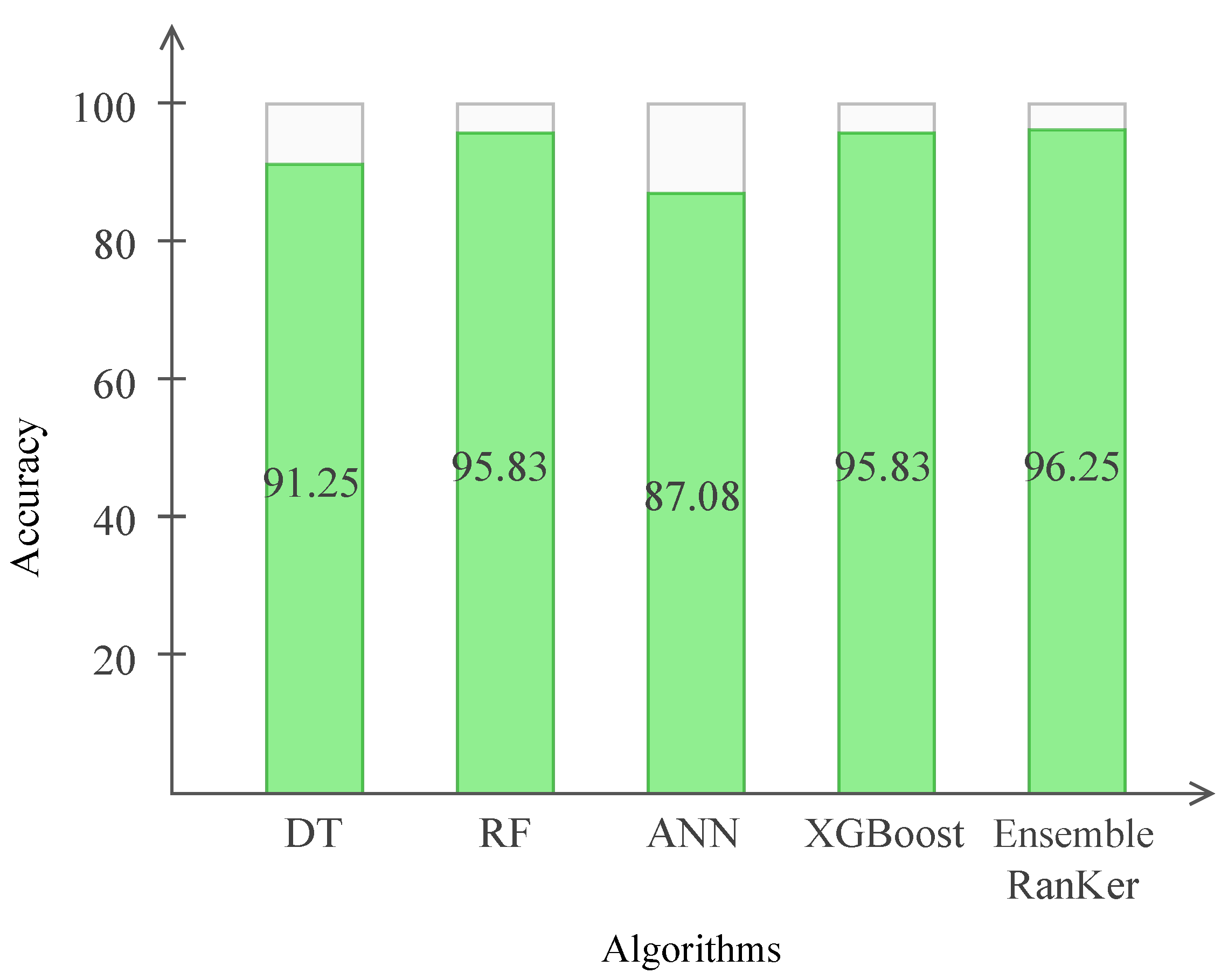
• A comparative analysis of various existing classification approaches such as RF, ANN, DT, XGBoost, has been conducted with the proposed approach, i.e., RanKer, to address the employee-performance classification problem.
• A novel ensemble-learning approach named RanKer combines with standard classifiers such as RF, ANN, DT, and XGBoost to predict an employee’s performance rating.
• Finally, the proposed model is analyzed for its performance using various AI-based evaluation metrics, such as ROC curve, confusion matrix, precision, recall, F1-score.

This article is divided into five sections. Section 2 discusses the related work. Section 3 presents the proposed approach for the classification of employees according to performance. Section 4 discusses performance evaluation for RanKer. Finally, this article concludes in Section 5 followed by discussion of future research work.

2. State-of-the-Art

Measuring employee performance and keeping track of skillful employees so that they are properly acknowledged is a prime concern for any organization. Various researchers have tried to measure the performance of employees with the help of prediction algorithms. However, many organizations still rely on human performance and still give performance ratings to employees manually, as there is a lack of a proper AI-based system predicting the performance of employees.

Table 1. Comparison of various existing approaches with our proposed method.

Author	Year	Approach	Results	Key Contributions	Cons
Ajit et al. [6]	2016	XGBoost Classifier	86% (AUC)	Utilized XGBoost Classifier for predicting performance turnover of employees and concluded that XGBoost classifier is a superior algorithm for predicting turnover	They have not considered the scalability.
Liu et al. [7]	2018	RF, SVM, LR and AdaBoost	86.3% (Accuracy)	Various AI-based prediction models are used to forecast staff turnover. Results show that expertise is the most influencing factor while predicting.	The proposed approach only focuses on one organization; they have not considered employee datasets from different organizations
Lather et al. [1]	2019	RF, SVM, ANN, LR and NB	85.3% (Accuracy)	Proposed a system after conducting standard tests for better prediction of employee performance and performed various ML algorithms for the same.	They have not considered feature’s correlation matrix.
Kamtar et al. [8]	2019	SVM, KNN, RF, DT, NB, Cascading Classifier and LR	90% (Recall) 80% (Precision)	Applied ML algorithms for employee performance prediction using DISC personality.Performance of Employee was predicted with the help of ensemble model.	They have not performed any statistical tests for the verification of their results.
Jayadi et al. [9]	2019	NB	95.48% (Accuracy)	Authors implemented NB for dataset of 310 employees and obtained significant results.	Not compared the results with other ML-algorithms.
Fallucchi et al. [10]	2020	Gaussian Naive Bayes, NB, LR, KNN, DT, SVM, Linear SVM	54.1 % (Recall)	Utilised various ML techniques to predict employee attrition. Models were trained and tested on a standard real-time dataset (given by IBM).	Adopted traditional ML algorithms; did not propose a novel approach.
Juvitayapun et al. [11]	2021	LR, RF, gradient boosting tree, extreme gradient boosting tree	98.03% (accuracy), 97.18% (precision), 90.79% (F1-score), and 85.19% (recall)	Extreme gradient-boosting algorithm gives best results that detect worker’s likelihood to leave an organization.	They have not discussed statistical tests.
Duan et al. [12]	2022	LR and XGBoost	98.17% (accuracy)	They involved Ml classifiers that predict employees’ tendency to leave enterprises.	No discussion on different performance evaluation metrics such as precision, recall, F1-score.
Sujatha et al. [13]	2022	XGBoost and gradient boosting	92.20% (accuracy)	The proposed scheme predicts employee performance in an MNC company.	They have performed statistical test and not calculated a correlation matrix.
Obiedat et al. [14]	2022	J48, RF, RBF, MLP, NB, and SVM	98.3% (Accuracy)	The proposed scheme predicts the productivity performance of garment workers.	They have not performed statistical tests.
Proposed approach RanKer	2022	Ensemble Learning (DT, RF, ANN, XGBoost)	96.25% (Accuracy)	Proposed an ensemble-learning approach for employee performance classification based on ratings by combining individual approaches such as DT, ANN, RF and XGBoost.	-

shows a relative comparison of the proposed ensemble-based RanKer model with the existing baseline approaches.

Recent works for employee performance classification include implementing various ML techniques. Various works aim to understand the effect of psychological, socioeconomic, and creativity factors on employees’ performance and commitment [15]. One such work was proposed by Lather et al. [1]. For prediction purposes, they used a self-made dataset using standard tests such as Abbreviated Torrance Test for Adults (ATTA), Thomas–Kilmann Conflict Model Instrument (TKI), Fundamental Interpersonal Relations Orientation Behaviour (FIRO-B), and Motivational Analysis Test (MAT). They then used it for training and testing purposes. Authors developed various ML algorithms such as RF, SVM, ANN, LR, and NB with 10-fold cross-validation.

Liu et al. [7] proposed an AI-based approach for prediction of employee turnover. The dataset was obtained from state enterprises, and employees’ job performance was taken. Feature extraction was performed to find the important factors that impact employee performance. A grid search was used to find the best features for the model. Classification methods such as RF, SVM, LR, and AdaBoost were applied to predict the turnover of an employee. Employee turnover predicts that the job skills and performance of an employee are directly co-related to each other.

Another work for prediction of employee performance was proposed by Kamtar et al. [8]. The sole purpose of this study is to efficiently classify employees’ job performance based on DISC personality. By observing the feature space and class label of the dataset, the problem was formulated as a multi-class classification (MLC) problem by defining job performance as class labels. The process model was divided into three steps, which are building an MLC model, applying a stack or an ensemble model, and then feature selection for selecting attributes that are important for final prediction [16]. They tested the model on a self-made dataset with a DISC personality test on 2137 employees. They also collected the last three years of job performance records and classified the job performance into four types. They compared the results of various classification algorithms such as SVM, k-NN, RF, LR, DT, NB, and cascading classifiers and provide the performance rating. Again, using ML algorithms, Jayadi et al. [9] developed a model using Naive Bayes for the employee-performance prediction for data mining. A dataset consisting of 310 employees was utilized for training and testing purposes.

An approach based on XGBoost classifier was proposed by Ajit et al. [6]. They evaluated the model on a self-made dataset taken from the HR Information Systems (HRIS) with 73,115 data points, with each labeled. The data points were passed into the feature-extraction process for selecting the features that most impact turnover. The main point was that the noise in the data was highlighted and removed during the process. The turnover prediction was made with the help of the XGBoost classifier. Then, Fallucchi et al. [10] proposed various ML approaches such as KNN, DT, SVM, Gaussian NB, LR, NB for multivariate Bernoulli models, RF, and linear-SVM to predict the employee’s decisions such as whether they will leave a company or not. For that, they analyzed and studied the objective factors that influence worker attrition. Moreover, they considered a correlation matrix for the features and performed statistical analysis. They performed a comparative analysis of various ML algorithms, and, after comparison, they claimed that the Gaussian NB classifier gives the best performance. Juvitayapun et al. [11] proposed LR, RF, gradient boosting tree, and extreme gradient boosting tree classifiers that detect a worker’s likelihood to turnover from the organization. In addition, Duan et al. [12] proposed LR and XGBoost that predicts the likelihood of employees leaving an organization. They performed a likelihood ratio test using the chi-square approach. Their simulation results show the XGBoost algorithm outperforms the LR algorithm in terms of accuracy. Further, Sujatha et al. [13] proposed an ML-based classifier such as XGBoost and gradient boosting. They worked on the real-time dataset of employee details for an MNC company. Then, Obiedat et al. [14] aimed to predict the productivity performance of employees in the garment sector. Therefore, they proposed a hybrid algorithm that merges multiple ML classifiers such as J48, RF, RBF, MLP, NB, and SVM. Moreover, they used different ensemble-learning algorithms such as Adaboost and bagging with classical ML classifiers. They considered accuracy, mean absolute error (MAE), and root mean square error (RMSE) as performance evaluation metrics. They obtained results using with and without Adaboost and bagging algorithms. After analyzing lots of literature, we observed that most of the authors focused on the classical ML algorithms, such as NB, RF, DT, SVM, etc. Many of them have not performed a statistical test on the results and have not considered the correlation matrix. As per our knowledge, we analyzed that they have not proposed any novel algorithm that predicts employee performance. Therefore, we proposed a novel algorithm, RanKer, for better and more efficient prediction of employee performance. Our system, RanKer, proposes an ensemble model of the classifiers combining RF, DT, ANN, and XGBoost and compares the result with the existing work. Further, we anlyzed the correlation matrix and performed statistical tests.

3. Proposed Approach

In this section, we elaborate the proposed methods for the classification of employee performance.

3.1. System Architecture

For the classification of employee performance, we have developed a system architecture in the form of a flowchart (as show in Figure 1) which shows the basic working of the system which begins with the considered employee performance dataset in which feature selection and scaling is applied to further perform the division of testing and training dataset. Further, conventional classification algorithms and the proposed approach is considered to train and evaluate the employee-performance ratings. Moreover, the dataset collection step was performed, then we selected the useful features from the available features in the dataset through the feature selection step. In addition, then, we used feature scaling to scale up the features. After that, the classification was performed using ML algorithms such as DT, RF, ANN, XGBoost, and AdaBoost. At last, we implemented a novel approach, RanKer, an ensemble-learning method, to achieve better results.

3.2. ML Classification Algorithms

In this section, we discussed various AI methods that we implemented to classify employee performance in the company.

3.2.1. Decision Tree (DT)

DTs are one of the most important and successful classifiers. A dataset is represented by a tree-like structure in DT [17]. DTs can process any data, discrete or continuous. DT can represent all boolean functions. A series of tests is performed where a test of the internal attribute is represented in the form of an internal node of tree [18]. This approach is very easy for humans to understand. DTs cause over-fitting if no pattern is found and result in many trees [19].

It helps by breaking a multistage approach to help make the union of simpler decisions in place of complex decisions [20]. These tree-based algorithms make it easy for the user to interpret and empower the classifying property to achieve high accuracy and stability. When a user has to achieve high accuracy, the DT helps. There are two types of DT: categorical based and continuous based on the target variable type. It places the best attribute at the tree’s root and is continued until we do not find all the leaf nodes. For that, we assign all training instances to the root of the DT; here, we have ten training instances (number of attributes). Each training instance provides information gain ratio using gain_ratio(), where we find the largest gain ratio attribute. Here, the minimum samples required for splitting an internal node were assumed as 5. These were chosen using the grid-search technique. For implementing the model, a random state of 42 was taken. Further, the splitting and Gini criteria were set based on the high gain ratio. Both terms identify the best splitting node from which the DT can split. Then, each individual split tree provides a prediction output.

3.2.2. Random Forest Classifier (RF)

RF is a variant of DT, which contains small decision trees that work as an ensemble [21]. Each decision tree in the forest gives its prediction, and the class predicted by a maximum number of trees is considered the output [22]. The reason behind the success of RF is that it has several unrelated trees that will outperform any model. Each classifier in the RF is generated using the random vector developed with the help of the input vector. Each tree in the forest has a unique vote for the vector generated [23]. Then, it uses arbitrarily selected features or combinations to grow a corresponding tree.

RF considers Gini Index as an attribute selection measure. It measures the feature importance for different classes. It contains multiple DTs, so it is also called an ensemble-learning method [24].

To improve the performance efficiency of the DT, we employed an ensemble approach of several DTs and an RF classifier. Similar to the approach of DT, we utilized the scikit learn library for implementing RF. Moreover, utilizing the averaging classifier enhances the prediction accuracy and efficiently manages the over-fitting problem. A total of 100 DTs were used in the forest as estimators, and a random state was taken as 33. To measure the quality of the splitting among the decided 100 estimators, a gini criterion was added. The minimum samples required for splitting an internal node and required at each leaf node were assumed as 4 and 1, respectively. These parameters were cross-verified using the grid search technique. Here, all training instances $\left(n\right)$ are given as input to the RF classifier, which provides output as a performance rating. First, the required number of estimators is set as $(t=100)$; then, from n instances, a total of 10 instances were randomly selected. Further, we calculate the node $\left(d\right)$ for splitting the tree using the optimal split point and Gini criterion. Using the node $\left(d\right)$, the nodes were divided into daughter nodes. Then, the target for 100 training instances was predicted and the votes for the same calculated; based on the maximum votes, the final prediction of the RF algorithm is evaluated.

3.2.3. Artificial Neural Networks (ANN)

The biological neural network which constitutes the brain inspired the ANN [25]. A neural network is formed of multiple neurons, as in our brain. The neurons in the body are interconnected and pass the signals in it from the brain to various other parts of the body. Approximately 100 billion neurons still exist in our body. In the body, electrochemical signals vary with dynamic conditions, while the signals in ANN are of a binary or a real number (based on the problem). The signals are formed by activation functions such as rectified linear unit (ReLU), tanh, etc. These signals are passed to another neuron as an input. The connection between neurons is known as an edge [26].

In ANN, all the neurons are usually aggregated into layers. The first and last layers are input and output layers, while the remaining layers in between them are hidden layers. The advantage of ANN is that it can adjust to data without being explicitly notified of a function or distribution [27]. ANN forms universal functional approximators. Moreover, it performs the classification process in three steps: forward propagation, backward propagation, and update parameters.

For implementing our dataset on the ANN model to classify employee performance, we used the MLP (Multilayer Perceptron) classifier of scikit learn library. We took the ReLu activation function for hidden layers as it bounds negative outputs to zero, thus resolving the problem of vanishing gradients that might occur while using the sigmoid or tanh activation function. Instead of using gradient descent, we used a mini-batch gradient descent algorithm that will divide the training set into mini-batches. Then, gradient descent would be applied in an individual mini-batch. This helped to build our neural network faster and more efficiently. The ANN algorithm first initializes using various parameters, such as X_train size = number of training instances, batch_size = 10, and learning_rate = 0.01. According to the batch_size(), the number of instances is fed as an input to the forward propagation of the ANN algorithm. In forward propagation, each batch provides predicted output for training instances using an activation function, i.e., $relu\left(\right)$ and $sigmoid\left(\right)$. Then, the backward propagation is applied to optimize the predicted output. At each iteration, the error of predicted output is minimized and the performance rating maximized.

3.2.4. XGBoost Classifier

XGBoost Classifier was proposed by Chen, and used in tree boosting. XGBoost uses the concept of gradient boosting, which works by combining weak learning models into a stronger learner [28,29]. Gradient boosting optimizes the loss function, and the residuals from the previous predictor will be optimized. XGBoost can be considered the perfect combination of software and hardware techniques which can provide great results in less time using fewer computing resources. XGBoost optimizes the system and algorithm using parallelization, regularization, pruning the tree, and cross-validation. It has higher prediction power than the RF classifier. The performances of employees was predicted with the help of the ensemble model. Algorithm 1 shows the implementation of XGBoost Classifier with the use of feature sets.

Then, we experimented with XGBoost classifier for employee performance classification. To implement it, we imported it from the XGBoost library (https://xgboost.readthedocs.io/en/latest/index.html, accessed on 21 May 2021). There are various boosters available, such as gbtree, gblinear, and dart. In our model, we used a tree-based model named gbtree. Again, 100 estimators were utilized similar to RF with a learning rate of 0.1.

Algorithm 1 XGBoost Classifier

Input: X, Employee Performance data. Input: r, Constrained DT Ratio. Input: K, The number of intervals according to feature sets. Output: Performance Rating P, $P\in \{0,1,2\}$. Procedure:   Calculating the degree of coorelation between the features in the data set which divides the feature interval.   while i < 100 do     using bootstrap to randomly select part of the sample data.     if $i⩽(r\ast T)$ then         generation of candidate feature sets         According to split node criteria, construction of DT         $i=i+1$     else         Random selection process to generate candidate features.         Generation of DT with the help of traditional RF algorithm.         $i=i+1$    end if   end while Prediction:   for $t=1$ to $test\_features$ do      Predict target for 100 created DT.      Consider final prediction of XGBoost Algorithm.   end for

3.3. RanKer: An Ensemble Learning Approach

3.3.1. Ensemble Learning

An ensemble-learning approach is a supervised learning algorithm as it can be trained and can be used to predict classes of data given as an input [30]. There are two families of ensemble class which are usually distinguished.

• Averaging methods: In this method, all the estimators are built differently and predictions of all of them are averaged [31]. This combined estimator is different than any other single estimator. The bagging method is an averaging method and it helps increase the accuracy.
• Boosting methods: Boosting tries to combine the weak models to make a powerful ensemble. This method focuses on the errors made by previous classifiers and tries to minimize these errors as in gradient boosting [32].

3.3.2. Implementation of RanKer Approach

After implementing the individual ML algorithms such as DT, RF, ANN, and XGBoost, to improve the performance of our employee classification problem, we implemented a novel approach named RanKer, an ensemble-learning approach which is the combination of previously implemented approaches such as DT, RF, ANN, and XGBoost.

For the implementation of RanKer, we utilized the voting classifier approach, i.e., $OneVsRestClassifier\left(\right)$, using the standard scikit learn library (https://scikit-learn.org/stable/modules/generated/sklearn.ensemble.VotingClassifier.html, accessed on  12 August 2022). We used all these four implemented algorithms as estimators by combining them into a hybrid model. The $OneVsRestClassifier\left(\right)$ uses $VotingClassifier\left(\right)$ to take input as estimators, which consists of all models (i.e., DT, ANN, XGB, RF). Here, we applied $voting{=}^{\prime }sof{t}^{\prime }$ so that the proposed approach uses voting based on the predicted probabilities of the output class. In the soft-voting classifier approach, the probability of included individual models is summed, and the prediction with the largest sum is selected [33]. In addition, it is possible to give more weight to certain models in comparison to other models while using the soft voting classifier. Then, $flatten\_transform$ is used to transpose the output predicted probabilities. Further, the estimator is forwarded for training purposes by using $fit(X\_train,y\_train).predict(X\_test))$. After training and testing the model on our dataset, we achieved an accuracy of 96.25%, which was higher compared to the conventional techniques we implemented before. The implementation of our RanKer approach is shown in Algorithm 2.

Algorithm 2RanKer: ensemble-learning approach

Input: X, Employee Performance dataset. Input: L, Learning Algorithm Utilized for RanKer. Input: W, Labels of the training dataset utilized. Input: N, Number of L used. Output: Performance Rating P, $P\in \{0,1,2\}$. Procedure:   ⟹ SET $N\leftarrow$ 4, i.e., number of L (DT, RF, ANN, and XGBoost learning algorithms).   ⟹ SET $C\leftarrow$ 3, i.e., classes in the training dataset.   for $i=1$ to N do     (1) Call L with $X_n$ and stores the classifier $L_n$.     (2) $Compare(W_n,C_n)$, where $C_n$ was generated from $L_n$. (3) Update the vote according to the comparison results. (4) Aggregate votes of the $L_{n}s$ to the ensemble approach RanKer.   end for Prediction:   for $t=1$ to $test\_features$ do     (1) Predict target for all $L_{n}s$ created for RanKer and $soft$ voting approach was utilized for finalizing the prediction.     (2) Consider final prediction of RanKer as output $P_t$.   end for

4. Result Analysis of RanKer

This section discusses the performance evaluation of the proposed approach by considering different performance parameters, such as accuracy, precision, recall, and F1-score. In addition, this section elaborates the underlying details of dataset, feature selection, and feature scaling.

4.1. Dataset Description

For the implementation of the proposed model, in this paper, we utilized a dataset of 1200 employees working in a INX Future Inc. company (https://github.com/AkshayDusad/Employee-Performance-Analysis, accessed on  7 June 2019). All the employees are categorized based on 28 various parameters. A few of these parameters are employee age, gender, marital status, job role, education level, job level, job satisfaction level, number of companies worked, employee work–life balance, employee department, attrition, and performance rating. The training dataset is fed to the AI model tested using the testing dataset. With the help of $train\_test\left(\right)$, the dataset is split into 80% for training and 20% as a testing set. The dataset consists of various attributes that directly and indirectly affect an employee’s performance rating. Here, the employee performance rating in the dataset is given in the range of 1 to 5, where 1 means low performance and 5 means outstanding. However, the employee-performance rating feature in the dataset is quite imbalanced, where employee ratings of 1 and 5 combined was only given to about 7% of the employees. This would make data imbalanced while performing predictions. Thus, employees with ratings of 1 and 5 were removed from the dataset. Therefore, an employee with performance rating 2 is given class 0, rating 3 is given class 1, and rating 4 is given class 2. Due to the increase in the number of attributes, there are high chances of an increase in training time, and, also, there is the risk of the over-fitting of the dataset. Thus, feature selection is required to reduce the total number of features while training by only considering important features that affect employee performance. This helped us to achieve better accuracy by a selection of the right subset of features according to their importance from

Table 2. Parameters considered for the classification of employee performance mentioned in the dataset.

Sr No.	Name	Description
Not included Features
1	EmpNumber	Unique id for every employee
2	Gender	(Male = 1, Female = 0)
3	Education Background	(Human Resources = 0, Life Sciences = 1, Marketing = 2, Medical = 3, Techincal Degree = 4, Other = 5)
4	MaritalStatus	(Divorced = 0, Married = 1, Single = 2)
5	BusinessTravelFrequency	(Non-Travel = 0, Travel_Frequently = 1, Travel_Rarely = 2)
6	EmpEducationLevel	(Below College = 1, College = 2, Bachelor = 3, Master = 4, Doctor = 5) Employee education level from 1 to 5
7	EmpJobInvolvement	(Very Low = 1, Low = 2, Medium = 3, High = 4, Very High = 5) Employee involvement level in job
8	EmpJobLevel	Employee job level in the current company
9	EmpJobSatisfaction	(Very Low = 1, Low = 2, Medium = 3, High = 4, Very High = 5) Employee job satisfaction
10	NumCompaniesWorked	Total number of companies employee has worked in
11	OverTime	NO = 0—not doing overtime YES = 1 Doing overtime
12	EmpRelationshipSatisfaction	(Very Low = 1, Low = 2, Medium = 3, High = 4, Very High = 5) Employee Relationship satisfaction
13	TotalWorkExperienceInYears	Total years of experience employee has
14	TrainingTimesLastYear	Number of times employee has completed training
15	ExperienceYearsInCurrentRole	Number of years in the current role
16	YearsSinceLastPromotion	Number of years since employee got last promotion
17	YearsWithCurrManager	Number of years the employee worked under the current manager
18	Attrition	(No = 0, Yes = 1)
Included Features
1	EmpDepartment	(Data Science = 0, Development = 1, Finance = 2, Human Resources = 3, Research & Development = 4, Sales = 5)
2	EmpJobRole	(Business Analyst = 0, Data Scientist = 1, Delivery Manager = 2, Developer = 3, Finance Manager = 4, Healthcare Representative = 5, Human Resources = 6, Laboratory Technician = 7, Manager = 8, Manager = 9 R&D, Manufacturing Director = 10, Research Director = 11, Research Scientist = 12, Sales Executive = 13, Sales Representative = 14, Senior Developer = 15, Senior Manager = 16 R&D, Technical Architect = 17, Technical Lead = 18)
3	DistanceFromHome	Distance from home to work
4	EmpLastSalaryHikePercent	Last percentage increase in salary (in %)
5	EmpWorkLifeBalance	Time spent by the employee between work and outside
6	EmpHourlyRate	Number of hours per week employee is working
7	ExperienceYearsAtThisCompany	Total number of years completed working at the company.
8	Age	Age of an employee = N
9	EmpEnvironmentSatisfaction	(Very Low = 1, Low = 2, Medium = 3, High = 4, Very High = 5) Employee environment satisfaction
10	Performance Rating	(Low = 1, Good = 2, Better = 3, Excellent = 4, Outstanding = 5) Employee performance in the company

.

In addition, we also visualized a few data columns and their influence on the performance rating of employees (Performance Rating is the class label). For instance, the performance rating is compared with employee hourly rate, employee experience at the company, age, and distance from home. Figure 2a shows the comparison of employee performance and employee hourly rate, where the employee (rating = 3) shows an average performance with hourly rate; whereas the employee (rating = 2 and 4) has less affect on hourly rate. Similarly, the dataset has employees who have experience up to 20 years in the same company (as shown in Figure 2b, there are a few employees who possess up to 40 years of experience. Further, Figure 2 illustrates the comparison of performance rating with age and distance from home).

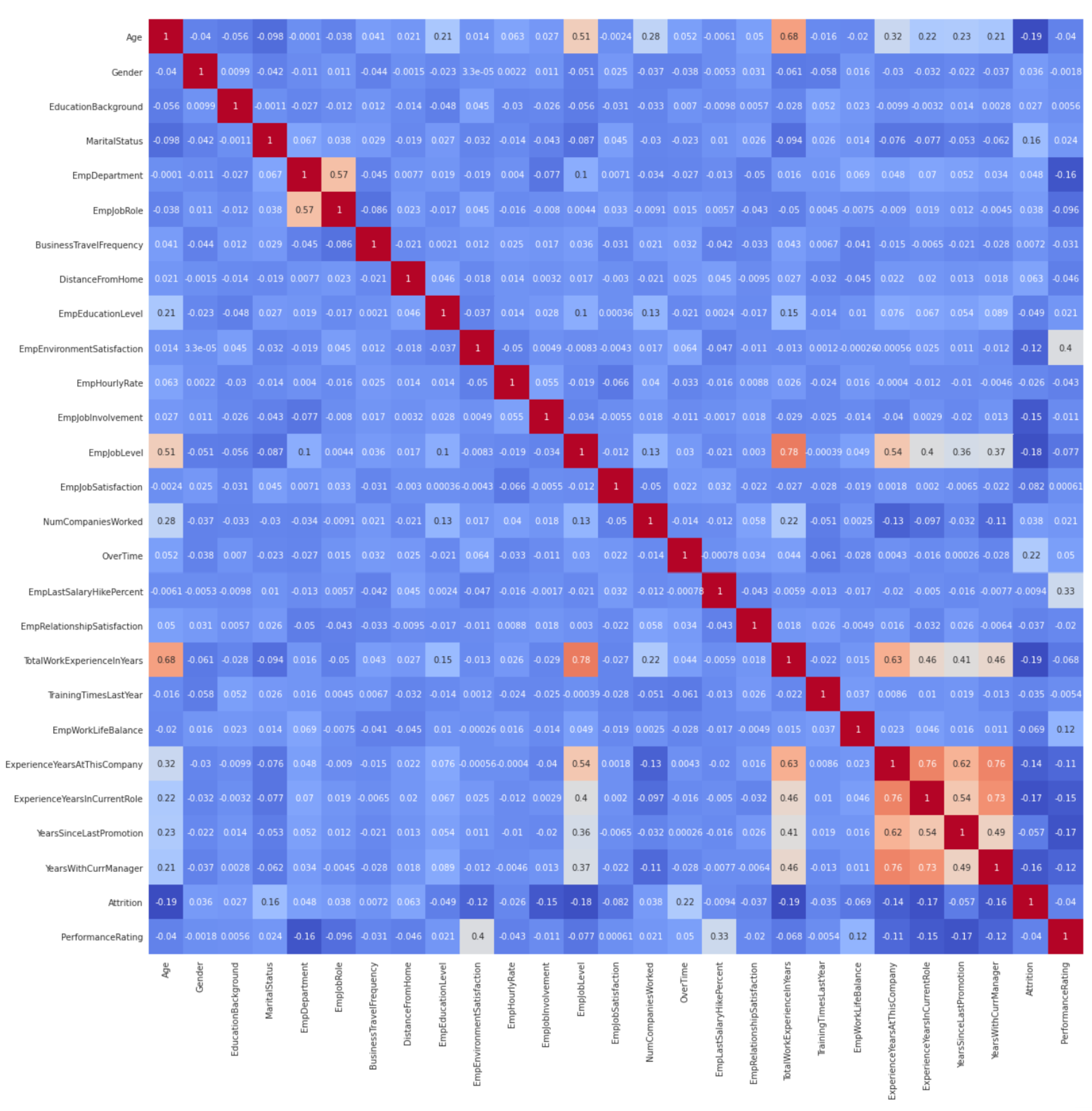
4.2. Feature Selection

The dataset contains 28 different features, including both direct and indirect features. To train our model on this dataset, we had to select the most significant and useful features affecting employee performance. Initially, we had to identify and eliminate those features from the final dataset that were becoming hindrances in training our model by increasing the training time and degrading the performance.

For this purpose, we observed some correlation between various features with the performance rating. Figure 3 represents the correlation matrix which shows how these features are correlated to each other. Based on the correlation values found, we decided to select the features whose correlation coefficient with a performance rating was more than 0.1. Furthermore, to validate the correlations, we applied principal component analysis (PCA) which provides a cumulative explained variance of our dataset. Figure 4 shows the explained variance acquired by each column of the dataset. It is clear from Figure 4 that ≈98% of information is created by the 20 features. However, when we train our models with 20 features, it shows overfit accuracies. Thus, we gradually lowered the features to 10 (has 76% of information) to achieve notable results in terms of accuracy, precision, and F1-score. Considering the mentioned correlation values and cutoff, we eliminated 17 features from the dataset and utilized the remaining ten useful features such as employee department, employee role in the company, distance of the company from employee’s home, employee environment satisfaction, percentage hike in employee’s last salary, employee’s work life balance, and many more.

Further analysing the dataset, we applied a few statistical tests to see the correlations between dependent and independent features. For that, we initially applied parametric tests to see the distribution of the dataset. From the Figure 5, we found that the dataset features are non-distributed (not showing the normal distribution); therefore, applying a non-parametric statistical test is appropriate.

We utilized the Mann–Whitney U test (see Listing 1) to show the measure of central tendency, i.e., median (as it is non-parametric) of the two columns of the dataset. Here, we used a significance of 0.05 to evaluate the null hypothesis, i.e., significant correlation between two columns of the dataset. If the p-value is smaller than the significance (i.e., 0.05), the null hypothesis is rejected.

Listing 1. Mann–Whitney U Test.

Further, we validated the Mann–Whitney U test with a chi-squared test that takes the same two columns, i.e., work experience of the employee and total work experience at the same company (we also measured other features while using statistical tests). We obtained a chi-square statistic (${\chi }^2$) value of 0.16295 and degree of freedom is 3. Based on the above-mentioned values, a p value is determined, i.e., 0.98333639, that rejects the null hypothesis, implying there is no significant correlations between the aforementioned columns.

4.3. Feature Scaling

After feature selection, feature scaling, i.e., a normalization technique, was applied to the dataset [34], which are like percentage hike in employee’s last salary, years of experience in current company, and others where there is a wide range of data values. In this case, if we apply ML algorithms, then the features with a broad range will dominate. Thus, feature scaling with the standard scaler method was applied to normalize all the features so that each selected feature contributes equally to the classification. In the standard scaler method, data in each feature is scaled so that the distribution of each feature is centered around 0 with a standard deviation of 1. Feature scaling using the standard scaler method was carried out using Equation (1).

$$x_{new}=\frac{x-\upsilon }{\sigma }$$

(1)

where x = individual value of the selected feature, $x_{new}$ = new value of selected feature after scaling, $\upsilon$ = mean of the selected feature, and $\sigma$ = standard deviation of the selected feature.

4.4. Evaluation Metrics

This section discusses various performance parameters we used to evaluate our model.

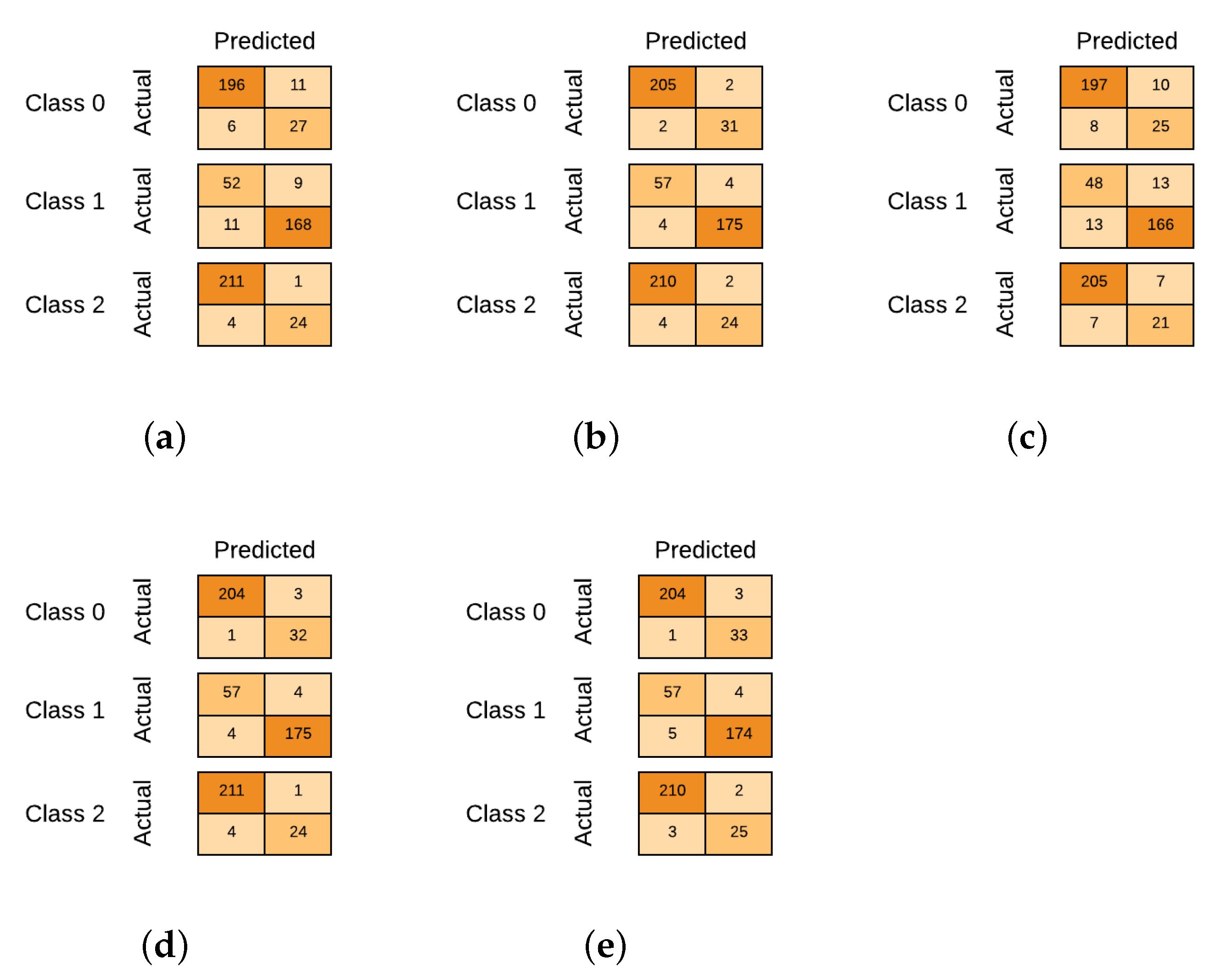
4.4.1. Confusion Matrix

A confusion matrix is a clean and unambiguous way to represent the model’s predictions. It comprises of four parameters, such as true positive (TP), false positive (FP), true negative (TN), and false negative (FN) [35]. Let us consider an example of a model which predicts whether a person has a performance rating of a particular class or not. A confusion matrix is given in Figure 6.

• True positive (TP): this is an outcome metric that aims to correctly predict the positive class, i.e., an employee performing well.
• True negative (TN): this is an outcome metric that aims to correctly predict the negative class, i.e., an employee not performing well.
• False positive (FP): this is an outcome metric that shows the model inaccuracy, i.e., the classifier model inaccurately predicts the positive class (employee performing well).
• False negative (FN): this is an outcome metric that shows the model inaccuracy, i.e., the classifier model inaccurately predicts the negative class (employee not performing well).

4.4.2. Recall

This specifies the number of actual positives correctly predicted by the AI model. Recall can also be known as sensitivity, as it is the probability of how many items selected are correct [16]. Recall alone is not enough to measure the predictability of the model, one also needs to measure the non-relevant predictions.

$$Recall=\frac{TP}{TP+FN}$$

(2)

4.4.3. Precision

This is the proportion of the number of actual positives that is correctly predicted by the model [36]. A precision score of 1.0 means that every input item predicted by the model to be of class C belongs to class C only. Precision is always used with a recall to measure the F1-score.

$$Precision=\frac{TP}{TP+FP}$$

(3)

4.4.4. F1-Score

This establishes a balance between the score values of precision and recall. It is a harmonic mean of precision and recall values [37]. A measure of the model’s accuracy can be performed by F1-score. In the case of uneven distribution, F1-score may be a better option to measure the predictability of a model rather than the accuracy.

$$F1-score=\frac{2\ast Precision\ast Recall}{Precision+Recall}$$

(4)

4.4.5. Regional Operating Characteristic Curve (ROC)

ROC curves displays the AI model’s performance by considering all classification threshold points. It comprises of sensitivity (true positive rate) and specificity (false positive rate); the curve has to make an efficient trade-off between specificity and sensitivity. The curve has two axis, i.e., sensitivity and specificity, wherein on the x-axis specificity and on the y-axis sensitivity are placed to depict all the classification thresholds. Moreover, two types of ROC curves exist: micro-averaged ROC curves and macro-averaged ROC curves. A macro-average computes all the metrics independently and then computes the average. The micro-average measurement will be performed by the contribution of all classes to compute the average metric.

4.4.6. Area Under the Curve (AUC)

One of the performance measurement curves for classification problems at various threshold settings.It measures the whole two-dimensional area under the ROC. It tells the degree of separability and how much the model can differentiate between classes. It is a scaled invariant as it measures the rank of predictions, not their actual values.

4.5. Performance Evaluation of the Ranker

This section discusses the performance of the proposed model by utilizing different performance parameters, such as accuracy, recall, precision, ROC curve, and F1-score.

4.5.1. Decision Tree

By implementing DT for our problem statement, we achieved 91.25% accuracy by testing it on our dataset. Figure 7a shows the confusion matrix for our model. Other evaluation metrics are shown in

Table 3. Evaluation metrics for DT, RF, ANN, XGBoost, and Ranker.

Classifier	Classes	Precision	Recall	F1-Score
Decision Tree	0	71%	82%	76%
	1	95%	94%	94%
	2	96%	86%	91%
Random Forest	0	94%	94%	94%
	1	98%	98%	98%
	2	92%	86%	89%
ANN	0	71%	76%	74%
	1	93%	93%	93%
	2	75%	75%	75%
XGBoost	0	91%	97%	94%
	1	98%	98%	98%
	2	96%	86%	91%
Ranker	0	91%	97%	94%
	1	98%	97%	97%
	2	93%	89%	91%

. Precision is 71% for the class-0 rating, 95% for the class-1 rating, and 96% for the class-2 rating. Recall is 82% for the class-0 rating, 94% for the class-1 rating, and 86% for the class-2 rating. F1-Score is 76% for the class-0 rating, 94% for the class-1 rating, and 91% for the class-2 rating. Figure 8a shows the ROC curve for this model, showing the curve for all three classes. AUC score for class 0 is 88%, for class 1 is 90%, and for class 2 is 93%.

4.5.2. Random Forest Classifier (RF)

We obtained the accuracy by using the RF model on our dataset, which was 95.833%. Figure 7b shows the confusion matrix for our model. Other evaluation metrics are shown in Table 3. Precision is 94% for class-0 rating, 98% for class-1 rating, and 92% for class-2 rating. Recall is 94% for class-0 rating, 98% for class-1 rating, and 86% for class-2 rating. F1-Score is 94% for class-0 rating, 98% for class-1 rating, and 89% for class-2 rating. Figure 8b shows the ROC curve for this model, showing the curve for all three classes. AUC score for class 0 is 96%, for class 1 is 96%, and for class 2 is 92%.

4.5.3. Artificial Neural Network

The accuracy we obtained using the ANN model on our dataset was 87.08%. Figure 7c shows the confusion matrix for our model. Other evaluation metrics such as precision, recall, F1-score are shown in Table 3. Precision is 71% for class-0 rating, 93% for class-1 rating, and 75% for class-2 rating. Recall is 76% for class-0 rating, 93% for class-1 rating, and 75% for class-2 rating. F1-Score is 74% for class-0 rating, 93% for class-1 rating, and 0.75 for class-2 rating. Figure 8c shows the ROC curve for this model, showing the curve for all three classes. AUC score for class 0 is 85%, for class 1 is 86%, and for class 2 is 86%.

4.5.4. XGBoost Classifier

While training the dataset on the XGBoost classifier, we obtained an accuracy of 95.833%. Figure 7d shows the confusion matrix for our model. Table 3 shows various performance evaluation parameters such as precision, recall, and F1-score for class 0, 1, and 2. The model achieves a precision value of 91% for class 0, 98% for class 1, and 96% for class 2. Further, the model obtained a recall value of 97% for the class-0 rating, 98% for the class-1 rating, and 86% for the class-2 rating. F1-Score is 94% for class-0 rating, 98% for class-1 rating, and 91% for class-2 rating. Figure 8d shows the ROC curve for this model, showing the curve for all three classes. AUC score for class 0 is %98, for class 1 is 96%, and for class 2 is 93%.

4.6. Ensemble Approach: RanKer

AI-based ensemble learning gives 96.25% accuracy when trained on the standard dataset. Figure 7e shows the confusion matrix for our model. Other evaluation metrics are shown in Table 3. The model achieves a precision of 91% for the class 0 rating, 98% for the class 1 rating, and 93% for the class 2 rating. Further, the model gets a recall of 97% for class 0, 97% for class 1, and 89% for class 2 rating. Similarly, F1-Score is calculated, i.e., 94% for the class 0 rating, 97% for the class 1 rating, and 91% for the class 2 rating. Moreover, the proposed Ranker is evaluated using a training and cross-validation score, where the training score specifies the accuracy score of the training dataset. To validate the accuracy of training dataset, we used cross-validation score using $validation\_curve\left(\right)$, which takes $mean$ and $standar{d}_{d}eviation\left(\right)$ of the training score. From the Figure 9, one can observe that at iteration 9, the training accuracy is ≈96.2% and validation accuracy is ≈91.34%. On further iterations, the gap between training and validation scores is going to be minimized and an optimal solution achieved.

4.7. Performance Comparison of RanKer with Other Methods

After implementing traditional ML and the proposed ensemble-learning RanKer, we compared their performance to find the best model. Figure 10 shows the accuracy measures of all the methods implemented on our test dataset for the employee-performance classification problem. It is clearly stated that RanKer has performed better than the other implemented methods by having an accuracy of 96.25%. RF and XGBoost come second by having an accuracy of 95.83% each. DT has also performed better by achieving 91.25% accuracy. While predicting employee-performance ratings, ANN has not performed up to the mark. From the above, it is concluded that our proposed ensemble approach works better when a huge number of parameters and features are considered for the employee-performance classification. Further, the proposed approach is evaluated using a log loss score, which specifies how close the predicted probabilities are to the ground-truth values. It also implies that the algorithm poses high accuracy, and must have a low log loss score. Here, the Ranker achieves 0.16477 log loss score value compared to other AI alogrithms (as shown in Figure 11). Thus, using this approach, the company could find low performers based on the parameters as stated in Table 2 so that the company could work to increase the working efficiency of the employees or can fire them, according to their requirements.

5. Conclusions

Performance analysis of employees is important for an organization’s growth, as manual analysis of employee performance is banal work. This highly complicated and tiresome process can be eased with the help of automation. Comparison of various methods for prediction of performance rating was carried out and, based on those methods, our ensemble approach RanKer was proposed. RanKer helps in the biased prediction of employee rating for an employee. Various pre-processing tasks such as feature selection and feature scaling were performed for the selection of the most affecting features to increase the performance speed and reduce over-fitting in our model. RanKer has performed far better than previous state-of-the-art approaches when tested on our test dataset. This approach obtained a 3–4% increase in accuracy over the previous state-of-the-art compared. Furthermore, we built ROC curves to analyze the model and visualize the result.

In the future, we can incorporate a decentralized mechanism with the proposed model to secure the AI-based classification to rank and identify low performers efficiently and reliably. For example, a malicious attacker can easily compromise employee data due to the data storage in an AI-based algorithm at a cloud server, which can be further accessed for manipulating or altering the data. Thus, it can reflect false information about the employee performance which affects the overall growth in organizations and can also discourage other employees who have been working hard for theor performance rating.

References

1. Lather, A.S.; Malhotra, R.; Saloni, P.; Singh, P.; Mittal, S. Prediction of Employee Performance Using Machine Learning Techniques. In Proceedings of the International Conference on Advanced Information Science and System, Singapore, 15–17 November 2019; Association for Computing Machinery: New York, NY, USA, 2019. [Google Scholar] [CrossRef]
2. Thakur, G.S.; Gupta, A.; Gupta, S. Data Mining for Prediction of Human Performance Capability in the Software-Industry. arXiv 2015, arXiv:1504.01934. [Google Scholar] [CrossRef] [Green Version]
3. Sasikumar, R.; Alekhya, B.; Harshita, K.; Sree, O.H.; Pravallika, I.K. Employee Performance Evaluation Using Sentiment Analysis. Rev.-Geintec-Gest. Inov. Tecnol. 2021, 11, 2086–2095. [Google Scholar] [CrossRef]
4. Alduayj, S.S.; Rajpoot, K. Predicting Employee Attrition using Machine Learning. In Proceedings of the 2018 International Conference on Innovations in Information Technology (IIT), Al Ain, United Arab Emirates, 18–19 November 2018; pp. 93–98. [Google Scholar]
5. Srivastava, D.K.; Nair, P. Employee attrition analysis using predictive techniques. In Proceedings of the International Conference on Information and Communication Technology for Intelligent Systems, Ahmedabad, India, 25–26 March 2017; Springer: Berlin/Heidelberg, Germany, 2017; pp. 293–300. [Google Scholar]
6. Punnoose, R.; Ajit, P. Prediction of Employee Turnover in Organizations using Machine Learning Algorithms. Int. J. Adv. Res. Artif. Intell. 2016, 4, C5. [Google Scholar] [CrossRef] [Green Version]
7. Liu, J.; Long, Y.; Fang, M.; He, R.; Wang, T.; Chen, G. Analyzing Employee Turnover Based on Job Skills. In Proceedings of the International Conference on Data Processing and Applications, Guangzhou, China, 12–14 May 2018; Association for Computing Machinery: New York, NY, USA, 2018; pp. 16–21. [Google Scholar] [CrossRef]
8. Kamtar, P.; Jitkongchuen, D.; Pacharawongsakda, E. Multi-Label Classification of Employee Job Performance Prediction by DISC Personality. In Proceedings of the 2nd International Conference on Computing and Big Data, Taichung, Taiwan, 18–20 October 2019; Association for Computing Machinery: New York, NY, USA, 2019; pp. 47–52. [Google Scholar] [CrossRef]
9. Jayadi, R.; Firmantyo, H.M.; Dzaka, M.T.J.; Suaidy, M.F.; Putra, A.M. Employee performance prediction using naïve bayes. Int. J. Adv. Trends Comput. Sci. Eng. 2019, 8, 3031–3035. [Google Scholar] [CrossRef]
10. Fallucchi, F.; Coladangelo, M.; Giuliano, R.; William De Luca, E. Predicting Employee Attrition Using Machine Learning Techniques. Computers 2020, 9, 86. [Google Scholar] [CrossRef]
11. Juvitayapun, T. Employee Turnover Prediction: The impact of employee event features on interpretable machine learning methods. In Proceedings of the 2021 13th International Conference on Knowledge and Smart Technology (KST), Chonburi, Thailand, 21–24 January 2021; pp. 181–185. [Google Scholar] [CrossRef]
12. Duan, Y. Statistical Analysis and Prediction of Employee Turnover Propensity Based on Data Mining. In Proceedings of the 2022 International Conference on Big Data, Information and Computer Network (BDICN), Sanya, China, 20–22 January 2022; pp. 235–238. [Google Scholar] [CrossRef]
13. Sujatha, P.; Dhivya, R. Ensemble Learning Framework to Predict the Employee Performance. In Proceedings of the 2022 Second International Conference on Power, Control and Computing Technologies (ICPC2T), Raipur, India, 1–3 March 2022; pp. 1–7. [Google Scholar] [CrossRef]
14. Obiedat, R.; Toubasi, S.A. A Combined Approach for Predicting Employees’ Productivity based on Ensemble Machine Learning Methods. Informatica 2022, 46, 1. [Google Scholar] [CrossRef]
15. Jay, P.; Kalariya, V.; Parmar, P.; Tanwar, S.; Kumar, N.; Alazab, M. Stochastic Neural Networks for Cryptocurrency Price Prediction. IEEE Access 2020, 8, 82804–82818. [Google Scholar] [CrossRef]
16. Verma, C.; Stoffová, V.; Illés, Z.; Tanwar, S.; Kumar, N. Machine Learning-Based Student’s Native Place Identification for Real-Time. IEEE Access 2020, 8, 130840–130854. [Google Scholar] [CrossRef]
17. Negnevitsky, M. Artificial Intelligence: A Guide to Intelligent Systems; Pearson Education: Upper Saddle River, NJ, USA, 2005. [Google Scholar]
18. Russell, S.; Norvig, P. Artificial Intelligence: A Modern Approach; Pearson Education: Upper Saddle River, NJ, USA, 2010. [Google Scholar]
19. Shah, H.; Shah, S.; Tanwar, S.; Gupta, R.; Kumar, N. Fusion of AI Techniques to Tackle COVID-19 Pandemic: Models, Incidence Rates, and Future Trends. Multimed. Syst. 2021, 1–34. [Google Scholar] [CrossRef]
20. Safavian, S.R.; Landgrebe, D. A survey of decision tree classifier methodology. IEEE Trans. Syst. Man Cybern. 1991, 21, 660–674. [Google Scholar] [CrossRef] [Green Version]
21. Ho, T.K. Random decision forests. In Proceedings of the 3rd International Conference on Document Analysis and Recognition, Montreal, QC, Canada, 14–16 August 1995; Volume 1, pp. 278–282. [Google Scholar]
22. Mistry, C.; Thakker, U.; Gupta, R.; Obaidat, M.S.; Tanwar, S.; Kumar, N.; Rodrigues, J.J.P.C. MedBlock: An AI-enabled and Blockchain-driven Medical Healthcare System for COVID-19. In Proceedings of the ICC 2021-IEEE International Conference on Communications, Montreal, QC, Canada, 14–23 June 2021; pp. 1–6. [Google Scholar] [CrossRef]
23. Pal, M. Random forest classifier for remote sensing classification. Int. J. Remote Sens. 2005, 26, 217–222. [Google Scholar] [CrossRef]
24. Breiman, L. Random Forests. Mach. Learn. 2001, 45, 5–32. [Google Scholar] [CrossRef] [Green Version]
25. McCulloch, W.S.; Pitts, W. A logical calculus of the ideas immanent in nervous activity. Bull. Math. Biophys. 1943, 5, 115–133. [Google Scholar] [CrossRef]
26. Patel, K.; Mehta, D.; Mistry, C.; Gupta, R.; Tanwar, S.; Kumar, N.; Alazab, M. Facial Sentiment Analysis Using AI Techniques: State-of-the-Art, Taxonomies, and Challenges. IEEE Access 2020, 8, 90495–90519. [Google Scholar] [CrossRef]
27. Zhang, G.P. Neural networks for classification: A survey. IEEE Trans. Syst. Man, Cybern. Part C Appl. Rev. 2000, 30, 451–462. [Google Scholar] [CrossRef] [Green Version]
28. Zhang, D.; Qian, L.; Mao, B.; Huang, C.; Huang, B.; Si, Y. A Data-Driven Design for Fault Detection of Wind Turbines Using Random Forests and XGboost. IEEE Access 2018, 6, 21020–21031. [Google Scholar] [CrossRef]
29. Friedman, J.H. Greedy function approximation: A gradient boosting machine. Ann. Stat. 2001, 29, 1189–1232. [Google Scholar] [CrossRef]
30. Polikar, R. Ensemble learning. In Ensemble Machine Learning; Springer: Berlin/Heidelberg, Germany, 2012; pp. 1–34. [Google Scholar]
31. Dietterich, T.G. Ensemble learning. Handb. Brain Theory Neural Netw. 2002, 2, 110–125. [Google Scholar]
32. Sewell, M. Ensemble learning. RN 2008, 11, 1–34. [Google Scholar]
33. Wang, H.; Yang, Y.; Wang, H.; Chen, D. Soft-Voting Clustering Ensemble. In Proceedings of the Multiple Classifier Systems, Nanjing, China, 15–17 May 2013; Zhou, Z.H., Roli, F., Kittler, J., Eds.; Springer: Berlin/Heidelberg, Germany, 2013; pp. 307–318. [Google Scholar]
34. Juszczak, P.; Tax, D.; Duin, R.P. Feature scaling in support vector data description. In Proceedings of the Proc. ASCI, Lochem, NL, USA, 19–21 June 2002; Citeseer: University Park, PA, USA, 2002; pp. 95–102. [Google Scholar]
35. Gareth, J.; Daniela, W.; Trevor, H.; Robert, T. An Introduction to Statistical Learning: With Applications in R; Springer: Berlin/Heidelberg, Germany, 2013. [Google Scholar]
36. Muhammad, Y.; Alshehri, M.; Alenazy, W.; Hoang, T.; Alturki, R. Identification of Pneumonia Disease Applying an Intelligent Computational Framework Based on Deep Learning and Machine Learning Techniques. Mob. Inf. Syst. 2021, 2021, 1–20. [Google Scholar] [CrossRef]
37. Tahir, M.; Khan, F.; Hayat, M.; Alshehri, M. An effective machine learning-based model for the prediction of protein–protein interaction sites in health systems. Neural Comput. Appl. 2022, 1–11. [Google Scholar] [CrossRef]
Figure 1. System architecture.
Mathematics 10 03714 g001
Figure 2. Comparison of performance rating with different columns of the dataset.
Mathematics 10 03714 g002
Figure 3. Correlation matrix.
Mathematics 10 03714 g003
Figure 4. Cumulative explained variance of the dataset.
Mathematics 10 03714 g004
Figure 5. Distribution of an individual data columns of the dataset.
Mathematics 10 03714 g005
Figure 6. Confusion matrix.
Mathematics 10 03714 g006
Figure 7. Confusion matrix comparison of the proposed scheme (a) DT, (b) RF, (c) ANN, (d) XGBoost classifier, and (e) ensemble learning: RanKer.
Mathematics 10 03714 g007
Figure 8. ROC Curve comparison of the proposed scheme. (a) DT, (b) RF, (c) ANN, and (d) XGBoost Classifier.
Mathematics 10 03714 g008
Figure 9. Train and cross validation of Ranker.
Mathematics 10 03714 g009
Figure 10. Comparison of current traditional ML approaches with proposed approach RanKer.
Mathematics 10 03714 g010
Figure 11. Log-loss score comparison.
Mathematics 10 03714 g011