Abstract
The traditional method of related commodity discovery mainly focuses on direct co-occurrence association of commodities and ignores their indirect connection. Link prediction can estimate the likelihood of links between nodes and predict the existent yet unknown future links. This paper proposes a potentially related commodities discovery method based on link prediction (PRCD) to predict the undiscovered association. The method first builds a network with the discovered binary association rules among items and uses link prediction approaches to assess possible future links in the network. The experimental results show that the accuracy of the proposed method is better than traditional methods. In addition, it outperforms the link prediction based on graph neural network in some datasets.
MSC:
68U35
1. Introduction
The most classic case of the related commodities discovery is the story of beer and diapers that happened in Walmart. Staff found that beer and diapers were often bought at the same time, so they placed them together. The case indicates that data mining technology can find interesting patterns from transaction data to improve commodity sales. Cross selling is a marketing method to meet customer needs and sell a variety of related services or products [,,], and a personalized recommendation system is used to recommend information and goods of interest to users according to users’ interest characteristics and purchase behavior, to realize cross sales. The most important task of cross selling is determining which items are most likely to be purchased together, that is, to find related commodities.
In cross selling, the most important method is association rule mining (ARM) [,,]. ARM is a common approach in data mining, which is used to mine the correlation between items. The most common application is to determine association rules from transaction data to discover the products that can be bundled together to increase sales. However, it can be determined which products are now co-occurring frequently. In fact, due to the accumulation of historical data, ARM cannot find new related goods in time, although people’s needs have changed. We also want to know which goods will appear in the same basket in the future. This cannot be solved by classical association rules mining.
The current studies on the items’ relationships in the shopping basket are mainly regarding next basket recommendation [,,] and sequential association rules [,]. Next basket recommendation focuses on finding preference changes from users’ historical baskets and purchasing sequences by creating shopper profiles and modeling a basket sequence for every user. The sequential association rule represents that a set of items usually occurs after a specific order sequence. Through modeling, one can find the temporal relationship between items and which products may appear in the user’s next basket. The effectiveness of the method mentioned above provides evidence for the evolution of products in the shopping basket; however, it is not easy to collect the purchase sequence of users for offline retail. ARM searches for interesting relationships between items by finding items that often appear at the same time in the transaction database. The purchase behavior of a small number of customers will not have a great impact on the results; however, the number may gradually increase over time. We need to find a way to discover these potentially related goods in advance.
Link prediction allows us to predict the future connection of nodes in the network in which new edges are the most likely to appear in the future [,]. As one of the research directions in the field of data mining, link prediction has been deeply studied. The initial direction of link prediction is to assist World Wide Web users to find web pages of interest from a large number of web pages []. With the continuous enrichment and development of link prediction, many researchers have applied it in many fields, such as community detection [], social relationships prediction [], features fusion in dynamic networks [], social network [,,], and biology []. In view of its great practical application value, we want to use it to find potential associated commodities based on current commodity associations. First, a commodity-related network is required to be built. In the current recommendation systems, some have built bipartite networks of users and products [,,]. A bipartite network is as follows: if there exists a partition such that , , and every edge connects a node of and an node of . In bipartite networks of users and products, and represent user set and product set, respectively. An edge indicates that a user has bought a product. For such a recommendation system, its main task is to find a series of interested products for every user. Collaborative filtering (CF) uses the user ratings to calculate the similarities between users or items and make predictions or recommendations according to their similarity values []. Using link prediction in bipartite graph networks requires mapping bipartite graphs into user networks and commodity networks [], and then calculating the similarity of the target user with users who bought enough of the same goods. Finally, the interest of the target user of different goods purchased by similar users is calculated. However, for the target user, it is not easy to find similar users and determine how many of the same products to buy. Because of the variety of goods, there are few of the same goods between different users compared with different goods. That is, the problem of data sparsity arises. Therefore, in this paper, the ARM is applied to find related commodities and build a network directly without purchase records of each user.
At present, there are few applications of association rules combined with link prediction, mainly graph association rule mining and multiplex link prediction []. They address multiplex link prediction via mining graph association rules. In this paper, we extend the usage of link prediction on a commodity network, and propose a potentially related commodity discovery (PRCD) algorithm based on link prediction. Link prediction adds new abilities to association rules mining. The motivations for our work are threefold: (1) We want to know which goods will appear in the same basket in the future. (2) We wish to find a way to discover potential related commodities based on the existing direct commodity association. (3) We look to uncover, in the absence of customer information, how to use link prediction to find related goods. This paper mainly includes three main aspects, as follows: (1) Construction of network. The commodity-related network is obtained by identifying all binary association rules from transaction data. (2) Selection of the best index. Finding the most suitable index for this network through experimental comparison. (3) Validation of the universality and superiority of the proposed algorithm, and running the proposed algorithm on different datasets and comparing it with other methods.
The proposed algorithm first builds a network with the discovered binary association rules among items and uses link prediction approaches in the network to assess possible future links. It has some advantages over the traditional methods, as follows: (1) Compared with other recommended systems, our proposed algorithm does not require any customer and commodity attribute information. This means less data processing and simpler algorithm design. (2) Compared with traditional link prediction, our algorithm improves the accuracy of the link prediction algorithm. (3) Compared with other network construction methods, our proposed method uses association rules to discover associations between items, thus building a network that can exclude unimportant and wrong links, to a certain extent.
The remainder of this paper is organized as follows. Section 2 introduces some related work about the recommender system, association rules, and link prediction. Section 3 describes classical link prediction concepts. Section 4 presents a potentially related commodity discovery (PRCD) algorithm. Section 5 compares the prediction accuracy and finds the best similarity index. In addition, the method in this paper is compared with other methods to prove its superiority. Finally, Section 6 summarizes the full text and presents the contribution, advantages, and disadvantages of this paper.
2. Related Work
This section reviews the research of the recommender system, association rules, and link prediction in recent years, which are related to the research topic of this paper.
2.1. Recommender System
When you log into the website of an electronic shop, irrespective of whether you have previously purchased anything on it, several products will pop up on the homepage. This is the result of a recommendation system that operates to reduce the cost of the query time required for users to search for products, thereby increasing the transaction rate of the website. Surprisingly, these recommended products are often similar to the products that a consumer has previously purchased or has been searching for. Obviously, the above system has the advantage of providing personalized recommendations. During the operation of the system, it will recommend products that are similar to the commodities that were previously purchased by the target customer or those purchased by other customers who have the same purchasing behavior as the target customer. In order to enhance the recommendation accuracy, the recommendation system depends on the consumption data [,,], opinion [], sentiment [], and consumption habits of the customer [,], even keeping track of the dynamics of customers’ preferences []. These recommendation algorithms are more suitable for personalized recommendation of long-term customers. Because there are enough data to train the algorithm, the recommended result is also good, but it cannot solve the problem of new users, and the cost of information collection is also high. In the field of time series data mining [,,,], Li [] used the techniques of sequence analysis to obtain sales correlations. Furthermore, Chen [] proposed a multi-kernel support tensor machine for classification to obtain cross-selling recommendations. They found that some commodities have sales correlation at some time points, and that sales correlation will persist for a certain time period. Through these methods, the recommendation system can not only know who to recommend what products to, but also know when to recommend. However, it is a problem to determine the time period. If the time segment is too long, effective information may be lost, but a short time segment may lead to a huge increase in the computation of the algorithm. In addition, there are many kinds of goods, so data processing is a big challenge. In the online retail industry, recommendation systems usually work well. However, uncertainty regarding the origins of customers has led to the fact that although offline retail shops store a large amount of transaction data, it is difficult to mine adequate information regarding the appropriate products required by a consumer from these data. Tracking the browsing trajectory of customers and collecting evaluation data and historical purchase data cost a lot. Moreover, the trend of customers paying increasing attention to their private data has also led to an increase in the difficulty of collecting information. Therefore, on the one hand, a recommendation system must be further developed that can enhance privacy without sacrificing accuracy [,]; and on the other hand, maintaining the accuracy of the recommendations based on fewer data requirements. In addition, novelty and diversity are also important for the evaluation criteria in recommendation systems [,], and some scholars also focus on recommending unexpected items to users []. For instance, when several customers purchase products A and B simultaneously, the system will recommend product B to the target customers who have purchased the product A. Conversely, when there is only a small correlation between products C and A, the system will not recommend C to target customers. For example, with classic beer and diapers, such rules have been excavated and applied because many users have already made such purchases, which means that this method cannot be used to discover these behaviors before they reach a limit. In this paper, we propose a method to try to find these frequent patterns before they can reach it.
2.2. Association Rules
Association rules reflect the interdependence and association between a thing and other things. Association rules mining (ARM) [] is a common approach in data mining which is used to mine the correlation between valuable data items from a large amount of data. Current research on ARM is not only focused on improving the efficiency of finding more interesting patterns [], but also applied to many fields, such as medical science [,], classification [], fault diagnosis, and anomaly detection [,,]. The apriori algorithm is an ARM method proposed in 1993 that was used to identify frequent rules and patterns from baskets []. In the whole algorithm execution process, all frequent itemsets can be found only by traversing the dataset twice. Many scholars have put forward improvement methods [,], while others have conducted further research to identify more meaningful patterns [,,]. However, we not only want to know which products are in the same shopping basket now, we also want to know which products may appear in the same shopping basket in the future. The problem cannot be solved with the classical method, so we focus on those indirect association rules.
The indirect association rule is the extension of the direct association rule. It was first proposed in 2000 []. The condition for an indirect relationship between commodities a and b is as follows: . Figure 1 illustrates the relation of a and b. Tan found that most of the products with indirect association rules are competing products by joining all frequent patterns. Although competitive product analysis is a research direction of commodity relationships, it is not helpful to find commodities in the same shopping basket, because competitive products generally do not appear in the same basket. Therefore, in the follow-up experiments, it is necessary to analyze whether there is a competing relationship for the potential related commodities discovered. Wan [] and Ouyang [] improved Tan’s method. Wan put forward an efficient algorithm HI-mine to mine indirect association for discovering a complete set. The main innovation of HI-mine is that it does not need to find all frequent rules. It also was utilized to find those pages that do not have indirect association but are often accessed together with a common set of pages []. In addition, Kazienko extracted indirect relationships between pages from historical user sessions and proved that indirect association rules can deliver useful information for a recommender system []. To the best of our knowledge, in recent years, few scholars have studied the use of indirect association rules, especially the indirect association of goods. Moreover, the indirect association rules previously studied by scholars have only one mediator, ignoring the case of multiple mediators. In addition, there is a lack of further research on the mediators, including the filtering of intermediary goods.
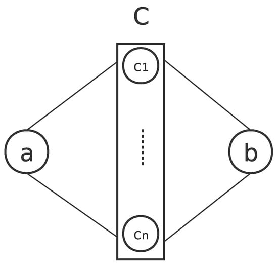
Figure 1.
Indirect association between a and b via a mediating itemset C.
2.3. Link Prediction
Classic link prediction methods mainly include similarity-based algorithms, maximum likelihood methods, and probabilistic models []. The first is based on node similarity and network structure. Despite its simplicity, it works very well on some networks. Maximum likelihood methods have good accuracy when dealing with networks with obvious hierarchical organization (such as terrorist attack networks). However, its computational complexity is very high, and it is not suitable for large networks. Probabilistic models not only use the network structure information, but also involve the node attribute information. They need to establish a set of adjustable parameters, and then use optimization strategies to find the optimal parameter values, so that the obtained model can better reproduce the structure and relationship characteristics of the real network. A probabilistic model can achieve high prediction accuracy. However, the disadvantages of this method are also obvious. Parameter adjustment is complex and time-consuming. The computational complexity and nonuniversal parameters limit its application. These methods that assume when two nodes are likely to link in advance are also called heuristic methods. When assumptions fail, the results will be very poor. In view of this, many scholars put forward that learning a suitable method from a network is a reasonable way, instead of using predefined ones. SEAL [] achieved state-of-the-art link prediction performance. It trains a graph neural network (GNN) on enclosing subgraphs around links to learn a heuristic. This can avoid inaccurate prediction caused by wrong assumptions, and even find new heuristics. Besides links in simple networks that describe pairwise interactions between nodes, hyperlink prediction aims to address interactions of arbitrary size in hypernetworks. HPLSF [] is the first hyperlink prediction method for a hypernetwork. It copes with association between multiple (more than three) homogeneous nodes by using latent social features. Later, many scholars put forward their improved methods, such as CMM [] and TF-DHP [], and Xiao [] considered hyperlink’s direction and the features of all entities. Since a hypergraph describes the complex relationship between multiple entities, it takes time to build a hypergraph and hence is expensive. Therefore, the shortage of training data becomes a big challenge for hyperlink prediction. In addition, traditional link prediction and evaluation methods cannot be directly used for hypergraphs. Determining how to generalize these methods to hypergraphs is also an urgent problem.
3. Link Prediction Based on Similarity
A link prediction algorithm based on similarity is the simplest and the most widely used algorithm. The assumption of the algorithm is that the more similar the two nodes are, the higher the possibility of creating a connection. In fact, the similarity between nodes is mainly calculated according to the graph structure features. The link prediction based on similarity includes local-information-, path-, and random-walk-based similarity indexes [].
An undirected network is defined as G = <V, E>, where V is the set of nodes and E is the set of observed edges. A is the adjacency matrix of the network, where = 1 if and , otherwise. The total number of nodes and connected edges in the network is denoted by K and L, and the maximum number of connected edges is , denoted by , where . A link prediction method is chosen to calculate the predicted value of each in .
3.1. Local-Information-Based Similarity Index
The similarity between nodes based on local information primarily considers the degree of nodes and common neighbors. The simplest index is CN, which only considers the number of common neighbors. If two nodes have more common neighbors, it implies that the nodes i and j are more similar and are more inclined to produce connected edges. In addition, LHN-I [], HPI, HDI [], Jaccard [], and PA [] consider the degree on the basis of common neighbors. AA [] and RA [] take the degree of common neighbors into consideration.
The degree of a node i is denoted as , and the neighbors of a node i are denoted as ; moreover, the set of CNs of nodes i and j is denoted as , where represents the number of CNs and . The definition formulas for local-information-based similarity index are summarized in Table 1.

Table 1.
Local-information-based similarity index.
3.2. Path-Based Similarity Index
The path-based similarity calculates the number of paths from node i to node j, and the shortest path is given more weight. is denoted as the number of paths of m order from node i to node j, and w represents the weight of the path. LP [] index only considers second- and third-order paths. The weight of the third-order path is w. If w is equal to 0, then the LP index is equal to the CN index. The Katz [] index considers all paths. is a decreasing coefficient and it is used to perform the role of adjusting the path. The expected number of paths of n-order between nodes i and j is denoted as , where is the maximum eigenvalue of adjacency matrix A. Table 2 shows the definition of path-based similarity index.
Table 2.
Path-based similarity index.
3.3. Random-Walk-Based Similarity Index
The similarity index of random walk calculates the average time required for different walking modes from node i to node j or the probability of node i reaching node j. Table 3 shows the definition of path-based similarity index. ACT [] and Cos+ [] assume that if the average commuting time of two nodes is smaller, the two nodes are closer. represents the average number of steps that are required to be taken from nodes i to j. . is regarded as the Laplacian matrix of the network, and is the pseudo-inverse matrix of . is the node degree matrix. RWR (random walk with restart) [] believes that every forward step has a certain probability x to return to the previous node. P is denoted as the Markov transition matrix of the network, and ( is an element in the adjacency matrix) is denoted as the probability that node i will move to node j. denotes the probability vector that node i reaches each node at time ( denotes the initial state vector; only the i-th element is 1; the remaining elements are 0). SimR [] is an index that indirectly conveys similarity. The primary idea is that if the neighbor of node i is similar to that of node j, the two are also considered to be similar. is a parameter of decreasing similarity. LRW (local random walk) [] is similar to SimR index; however, it limits the number of random walks and only calculates the probability that the node i reaches node j at the specified time . (initial state) is defined as the probability that node i reaches each node j at time . SRW (superimposed LRW) [] adds the value of obtained at all times of LRW.
Table 3.
Random-walk-based similarity index.
3.4. Weight-Based Link Prediction Index
Edge weight is a significantly important piece of information that describes the association between nodes in the network. The correct use of weights can improve the accuracy of the link prediction algorithm. W is a weighted adjacency matrix (the nonzero elements in the adjacency matrix A are changed to the value of the weight. Then, the weighted adjacency matrix is obtained). The contents as shown in Table 4 are certain similarity indexes based on the local information while considering weights [].
Table 4.
Weight-based link prediction index.
The parameter is used to adjust the weight. When is equal to 0, the weighted indexes are equivalent to their respective unweighted indexes. represents the total weight of node i.
4. Potentially Related Commodity Discovery Algorithm
In order to find the potential association between commodities, this paper proposes a PRCD algorithm based on link prediction. The algorithm assumes that as the similarity between commodities increases, the more likely it is that they will be appear in the same basket. This paper studies the future relationships based on current commodity relationships. Therefore, the experiment mainly includes the following two steps. (1) Find all binary association rules from transaction data, and build a commodity-related network according to association rules. (2) Calculate the similarity between commodities that do not have edges in the network in different ways, and predict which commodities may appear in the same shopping basket by comparing some indexes. Next, we will introduce them in detail.
4.1. Network Construction
In order to study the potential relationship between commodities based on these direct relationships, the association rule graph needs to be transformed to treat goods as nodes. A commodity-related network is defined as G=<V,E>, where V is the set of commodities which show in rules, and E represents the association of commodities. An adjacency matrix A is used to represent network structure. As shown in Algorithm 1, the apriori algorithm firstly returns the association rules. Then, an adjacency matrix A is constructed. If there is a rule , set and . In addition, if the indexes, such as WAA, take the weight into consideration, can be assigned other weight values. At last, Algorithm 1 returns adjacency matrix A.
| Algorithm 1. Build commodity-related network (BCRN). |
Retail transaction data: Parameters of association rules:
Adjacency matrix: A
|
4.2. Prediction Evaluation
After the network is built successfully, it is necessary to predict which commodities may appear in the same shopping basket in the future. Our hypothesis is that the higher the similarity between goods, the more likely they are to appear in the same shopping basket. It is necessary to test the correctness of this hypothesis and evaluate the prediction accuracy of each index. To evaluate algorithms, the data are usually divided into two parts: the training set and the probe set . In this paper, the AUC, precision, and RS [] are used to measure the accuracy of the link prediction. Among these methods, AUC is a metric to measure the accuracy of the algorithm with respect to the overall network prediction; moreover, it is also the most widely used. The RS calculates the ranking of all edges in . In contrast, the precision only focuses on the prediction accuracy of the top l edges.
For example, in Figure 2, the subgraph A indicates a network that contains eight nodes and 12 edges. , . First, four edges are randomly removed, as shown in subgraph B, and the network is divided into a probe set and training set . Then, the algorithm is executed in the training set , and each nonexisting edge (as shown by the dotted and red edges in subgraph C) obtains a similarity value . Second, one dotted line and one red line in subgraph C are randomly selected, and the similarity values of the two are compared. If the similarity value of the red line is bigger than the dotted line, ; if the similarity values are equal, . After comparison, the AUC is divided by the number of times of the comparison. Finally, the similarity of nonexistent edges is sorted. If there are m edges out of the top l edges in , then . .
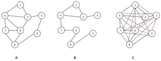
Figure 2.
Example of a commodity network. (A) is a complete network. (B) is a network with 4 edges randomly deleted. The dotted line in the (C) network represents the non-existent edge, and the red line represents the randomly deleted edge.
For each index, the specific steps for calculating the AUC, precision, and RS are shown in Algorithm 2.
(1) First, we obtain the set of edges E and set of nonexisting edges from network G. denotes the number of edges. (2) According to a certain proportion, the sample (, E) function can return a probe set . For example, if is 100 and the is 10%, then we obtain 10 randomly selected edges from E. (3) We calculate of each edge from and . , where , {, , , -I, , , , , , , , , -, , , , , , , , , }. For each , we can obtain the similarity matrix . (4) We randomly select an edge from and . If the of is more than that of , then 1 is added to the ; if the values are equal, then 0.5 is added to the . (5) We repeat step (4) n times, and finally . (6) The function Sort() sorts the edges according to similarity from the largest to smallest value and returns the matrix. The rank of is denoted by ( ). Then, the is calculated as
where and represent the number of edges in the probe set and the nonexisting edges set, respectively. (7) If there are m out of the top l edges in , then .
| Algorithm 2. Calculate , , and . |
Adjacency matrix: A Proportion of the probe set: Number of comparisons: n l of Precision: l Similarity index:
, ,
|
The best index was denoted as . The potential related commodities algorithm is shown in Algorithm 3. In this algorithm, the input is transaction data, and the outputs are potential related commodities of each commodity in rules. (1) Association rules are obtained by apriori algorithm. (2) The commodity-related network is built. (3) The similarity between all goods without direct correlation are calculated. (4) For each good in the rules, the top N items with the highest similarity are found. represents a vector that contains the similarity between commodity and other commodities that are not directly related. returns the top N commodities set
| Algorithm 3. Potential related commodity discovery algorithm (PRCD), cset = PRCD . |
Retail transaction data: Parameters of association rules: the top N commodity set: N
potential related commodity set:
|
5. Experiment
The experiments are implemented with a Windows 10 system on the Intel Core i5-4210u with 500 GB hard disk memory. Moreover, the related programs are compiled with Rstudio 1.2.5033 and Matlab R2012b.
When a lot of transaction data are collected, as shown in Table 5, it is easy to obtain association rules by apriori. The dataset OnlineRetail used in this pager is an open-source retail commodity sales dataset that can be downloaded from the UC Irvine website. Quantity, InvoiceDate, UnitPrice, and Country were removed. All commodities with the same InvoiceNo are a set of commodities purchased at the same time. When parameters are set as , the apriori algorithm is used to obtain 809 binomial association rules. Table 6 lists 10 association rules. The LHS column indicates the antecedent of the association rule; the RHS column indicates the consequent of the association rule; indicates the number of times the two commodities are purchased together.
Table 5.
Retail sales data Online_Retail.
Table 6.
Examples of association rules (sup = 0.008).
Figure 3 shows a graph for 300 rules, and rules are represented by nodes. The size increases with the increase of support, and the color of nodes deepens with the increase of lift. From the association rule graph, it can be found that commodities are clustered together.
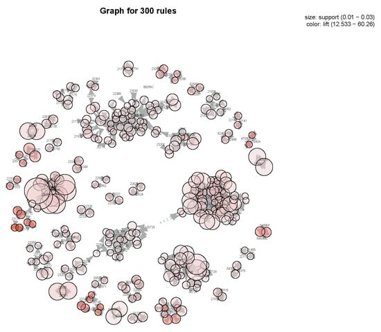
Figure 3.
Graph for 300 rules.
The accuracy of the same prediction algorithm in different networks may differ. To learn the prediction accuracy of different similarity indexes in different commodity-related networks, in the experiment of our study, three networks were generated. When , Algorithm 1 returns a matrix A, and the A is input into gephi to obtain the network, as shown in Figure 4a. Connected subgraphs are distinguished by colors. Link prediction is based on the connectivity of the network, so the maximal connected subgraph is retained, and the others are deleted, as shown in Figure 4b. Similarly, when set and , networks A, B, and C are commodity-related networks obtained, shown in Figure 5. The nodes represent the commodity and the label on the node is the StockCode. The larger the node, the greater the degree of the commodity, and more commodities have a strong association with it. In the association rules, the lift value is used to indicate the relevance of the two commodities and can be used to measure the strength of the association relationship. The count value indicates the number of times two commodities appear at the same time. To a certain extent, the two different values can be used as the weight of the connected edges in the commodity network. In Figure 5, the weight of the connected edges uses the lift value. As the lift value between the commodities increases, it indicates a stronger connection between the nodes. Table 7 lists the network topology of commodity associations under different support conditions.
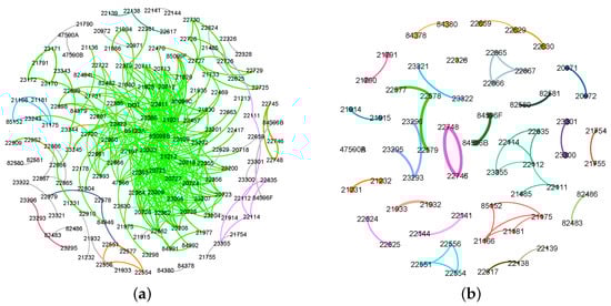
Figure 4.
Commodity-related network including all nodes (sup = 0.01). (a) shows that all nodes and connected subgraphs are distinguished by colors, while (b) displays nodes that should be deleted.
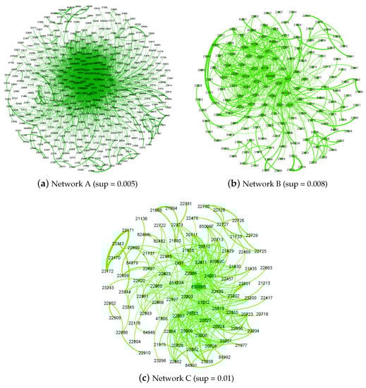
Figure 5.
Commodity-related network.
Table 7.
Commodity-related network topology under different degrees of support.
5.1. Comparison of Prediction Accuracy
To improve the prediction accuracy of the PRCD algorithm, it is necessary to find the best similarity index of the commodity association network. Therefore, it is essential to evaluate each index and determine which one will have higher prediction accuracy in different commodity networks. Different similarity indexes may have different prediction accuracies in networks A, B, and C. To determine the optimal similarity index and its characteristics in different commodity networks, the prediction accuracy based on different similarity indexes is compared in the subsequent section. Table 8 shows AUC of similarity index in different networks, when the proportion of the probe set is 10%.
Table 8.
AUC of similarity index in different networks.
5.1.1. Similarity Index Based on Local Information
When calculating AUC, the partition ratio and randomness of the probe set and training set may influence the result. For example, for each proportion of the probe set, random divisions are conducted 50 times. Then, the changing trend of that pertaining to the CN index is shown in Figure 6. The X-axis represents the number of times the experiment was conducted, and the Y-axis represents the AUC. Each broken line represents the impact of a random division on the AUC when the proportion of the probe set is provided. It can be observed that the AUC fluctuates around a number and does not fluctuate significantly. After conducting several experiments, it was determined that the AUC trend of other indexes is similar to the CN index. Therefore, in the following experiment, to avoid accidental factors, each calculated AUC was considered as the average of 20 random divisions.
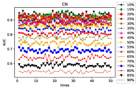
Figure 6.
Impact of random division on the area under the receiver operating characteristic curve (AUC) of common neighbor (CN) index for varying proportions of the probe set.
Figure 7 shows the AUC changes of the similarity index based on local information when the training and test sets are divided in different proportions. The X-axis is the proportion of test sets and the Y-axis is the AUC. Each broken line represents the trend of the AUC of the index corresponding to the changes in the probe set. The following aspects can be observed in networks A, B, and C. (1) The optimal value of AUC reaches 0.9 or more; moreover, the optimal value is not significantly different in each network. (2) The RA and AA indexes demonstrate the best performance in each network; further, the AUC gradually decreases as the proportion of the probe set increases. (3) The PA index is special. When the proportion of the probe set is less than 60%, the AUC value is relatively stable and is less than most of the other indexes. Moreover, it shows a marginal decrease when the proportion of the probe set is greater than 60%, but this change is better than that of the remaining indexes. This shows that the PA index still performs well under the condition that most of the side information in the commodity network is missing. It also shows that irrespective of when the purchase occurs, popular commodities are highly likely to be purchased at the same time. In the recommendation system, recommending commodities with higher popularity has a certain effect, especially when the information collection is insufficient. However, this method is not applicable to personalized recommendation systems. (4) In Network A, HDI is better than HPI. However, in networks B and C, this is not obvious. (5) The AUC of each index also decreases at different rates as the proportion of the probe set increases. The rate of decline is the slowest in Network A, followed by Network B, and it is the fastest in Network C. Table 8 lists the AUC of each index in different networks. In a network transformed by association rules with lower support, the optimal AUC of each index is relatively higher. The PA index has the largest change in the optimal AUC among the three networks, indicating that the AUC of this index is significantly affected by the network structure.
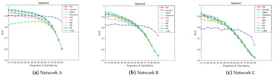
Figure 7.
AUC trends of similarity indexes based on local information when the proportion of the test sets increases.
Figure 8 shows the precision of the CN index. The X-axis indicates the value of l, and the Y-axis represents the precision. Each broken line represents the change in precision as the value of l increases for a given proportion of the probe set. When calculating the precision, l must be considered, because as l increases, the edge in the probe set is more likely to be in the top l. Therefore, 10 different values of l were set for each probe set. It can be seen that when the proportion of the test sets is low, the precision achieves its highest point when l is the smallest, which implies that the CN index is more accurate for predicting the top edges. However, with the increasing values of l, the precision gradually decreases. This shows that the prediction result is not good for edges that are ranked lower. When the proportion of test sets is high, the precision of the CN index reaches its apex when the value of l is maximum. This shows that the ranks of the edges in the probe set are lower. Then, we determined if the precision of all indexes have the same trend as the CN index. Figure 9 shows the precision of the similarity indexes based on local information, and the proportion of the probe set was set as 10%. Overall, the trend of CN, AA, PA, RA indexes, and HPI are similar. The precisions of others are relatively low, irrespective of the value of l. In addition, although the AUCs of HPI and HDI are not significantly different among the three networks, the precision of HPI is higher.
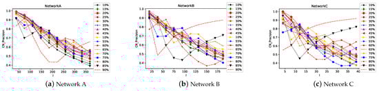
Figure 8.
Precision trend of CN corresponding to the increase in l.
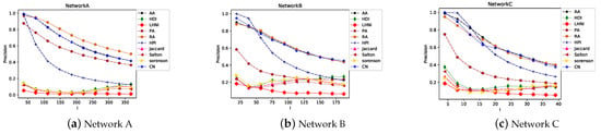
Figure 9.
Precision trend of different similarity indexes based on local information corresponding to the increase in l when the proportion of test sets is 10%.
The RS considers all the edges. The smaller the RS, the higher the edge ranking in the probe set. As Figure 10 shows, the values of the RS of the RA and CN indexes are smaller than those of other indexes; thus, it aids in maintaining a stable state. The difference of each index is more obvious in Network A. Although the precision of the PA index in Figure 9 is higher than several other indexes, the trend of the RS indicates that the overall ranking predicted by the PA is low. Moreover, the RS of HPI is marginally higher than HDI in networks A and B, but it is not obvious in Network C.
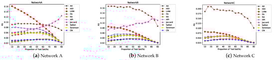
Figure 10.
Ranking score (RS) trends of similarity indexes based on local information corresponding to the increase in the proportion of the probe set.
5.1.2. Path-Based Similarity Index
Because the LP index considers second- and third-order paths, to determine whether adding a third-order path can improve the prediction accuracy, different values of weight w were considered. As shown in Figure 11, when the weight w of the third-order path changes, the AUC value changes significantly. When w is less than 0, the AUC value stabilizes at a lower level. However, when w is more than or equal to 0, the AUC suddenly increases, reaching the maximum value, and then remains stable. Although the changing trend of AUC is the same in the three networks, the change range is different. The largest change is observed in Network A, followed by in Network B, and finally in Network C. This shows that the weight of the third-order path has a significant impact on the network.
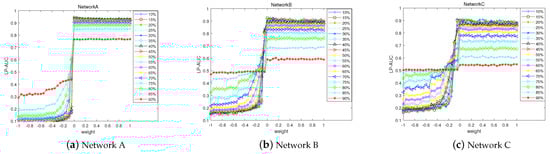
Figure 11.
Influence of third-order path weights on AUC of local path index.
As the CN index only considers the second-order path, to further study the role of the third-order and longer paths in the commodity association network, the similarity indexes based on the path were compared with CN. As shown in Figure 12, at the beginning, the AUC values of the similarity indexes based on the path are marginally less than that of the CN index, which shows that the second-order path performs a larger role in transmitting similarity in the network. A longer path will weaken this effect. It can be observed that as the proportion of the probe set increases, the AUC of the CN index decreases faster and is lower than Katz and LP indexes, which indicates that the indexes based on the global path perform better if there is more information missing. The AUC of LHN-II is maintained at 0.5, indicating that this index is not applicable in commodity networks.
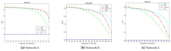
Figure 12.
AUC trend of the path-based similarity indexes and CN index when the proportion of the probe set increases.
Figure 13 and Figure 14 show that the CN index has higher precision and lower RS than the path-based similarity indexes. Moreover, the RS of the LP index is lower than that of the Katz index. Table 8 shows that the maximum AUC of the CN index is 0.95, and that of the LP index is 0.93. Therefore, the accuracy of prediction cannot be improved by considering more or all paths.
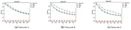
Figure 13.
Precision trend of the path-based similarity indexes and CN index when l increases.
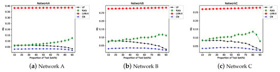
Figure 14.
RS trend of the path-based similarity indexes and CN index when the proportion of the probe set increases.
5.1.3. Similarity Index Based on Random Walk
The RWR index assumes that every step to the next step has a certain probability x of returning to the previous node. In a commodity association network, x can be considered as the probability of repeated purchases after a customer purchases a certain commodity. To study the effect of x in the commodity network on the AUC of the RWR index, x was set to range from 0.1 to 0.9. The results are shown in Figure 15. The X-axis indicates the proportion of the probe set, and the Y-axis indicates the AUC. Each broken line represents the change in AUC when x is provided. For the different values of x, there is no significant difference in the AUC of the RWR index. Therefore, the changes in x will not affect the AUC. In Network A, RWR has the highest AUC.
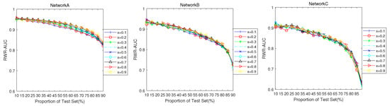
Figure 15.
AUC trend of random walk with restart index in different networks corresponding to changes in the return probability x and proportion of test sets.
Different networks may be required to set different steps to achieve the best prediction accuracy. As shown in Figure 16, the change in the steps makes the AUC of the LRW and SRW indexes first show an upward trend, and then it tends to stabilize. However, based on the changes in the proportion of test sets, the steps until the AUC achieves an optimal value are also different. When the proportion of the probe set is relatively low, the apex is achieved in two or three steps; when the proportion of test sets is higher, the steps required for the AUC to reach the peak value are also relatively more. This result is consistent with the AUC change trend of the path-based similarity indexes. In addition, the AUC of indexes based on the LRW is higher than others under the condition that the probe set occupies a relatively high level, predominantly reaching a value of more than 0.8, indicating that the LRW and SRW indexes are more suitable when a large amount of information is missing or when the information collection is not sufficiently comprehensive.
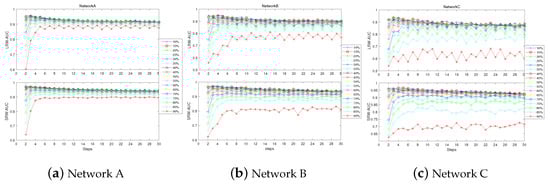
Figure 16.
AUC trend of local random walk index corresponding to the changes in the number of steps.
From the Figure 17, it can be noted that the LRW-based indexes perform better than the global random walk indexes. Moreover, the LRW-based index time complexity is lower than the global random walk index but higher than the similarity index, based on local information and path. Among the indexes based on LRW, the SRW index has a higher AUC than LRW. It can also be observed from Figure 16 that the AUC trend of SRW is more stable. In Figure 18, the precision of the similarity index based on random walk is lower than others. The maximum value is only 0.4. Especially for SimR, among the top l edges, there are no edges in the probe set.
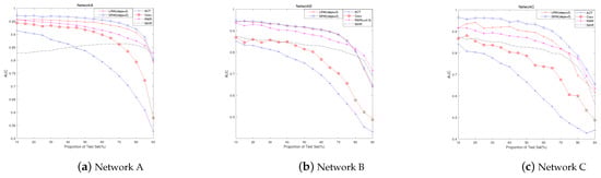
Figure 17.
AUC trend of similarity index based on random walk in different networks when the proportion of the probe set increases.
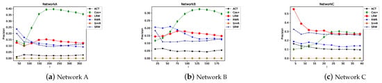
Figure 18.
Precision trend of similarity indexes based on random walk when l increases.
In Figure 19, the RS of LRW and SRW is maintained at approximately 0.05 and is higher than that of the indexes based on local information. Although the AUC of the similarity indexes based on random walk is high, the edges in the probe set are not ranked ahead of the nonexiting edges. Therefore, when these indexes are used to calculate similarity, the inaccurate results are easy to obtain when selecting the top N products.
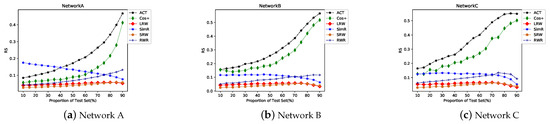
Figure 19.
RS trend of similarity indexes based on random walk when the proportion of the probe set increases.
5.1.4. Weighted Similarity Index
When the association rules are converted to the network, both the lift and count can be used as a weight to measure the strength of the association relationship of the commodities. To determine which of the two is more suitable for similarity calculation, experiments were conducted separately. The parameter is used to adjust weight. The continuous increase in implies that the weight performs an increasing role in the calculation process. If the weight is less than zero, it implies that the weight has a negative effect. If is greater than zero and less than one, it implies that although the weight has a positive additive effect, the effect is weak. If is greater than one, it implies that the effect is greater. Figure 20 shows the AUC changes when the adjustable parameter increases. The following aspects can be noted from this figure. (1) It can be observed that the AUC in different networks all reach more than 0.9 and there is no obvious difference between them. (2) As increases, the AUC of WCN has a marginally upward trend, especially in Network A. However, from Figure 20, it cannot be judged which parameter, i.e., lift or count, is significantly better as a weight. (3) As Table 8 lists, the AUC of weighted index is higher, indicating that the effective use of weight information can improve the prediction accuracy. Moreover, the WAA achieves the highest AUC of 0.9682.
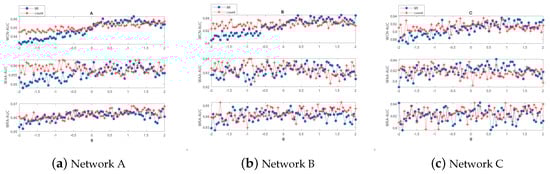
Figure 20.
AUC trend of weighted similarity index in different networks when increases.
Figure 21 and Figure 22 clearly show the impact of on the precision and RS. When the proportion of the probe set is 10% and , for WCN and WRA, as increases, the precision increases and RS decreases. This trend is more obvious in Network A. This indicates that the appropriate use of weight is also beneficial for precision and RS. However, when increases, the precision and RS of WAA demonstrate an upward trend. Figure 23 shows that the precision trend of the weighted index is similar to that of the original index. When , the precision values of WRA and WCN are higher than those of RA and CN. In Network A, based on the precision and RS, it can be considered that WRA is better than WCN. However, in networks B and C, WCN is better than WRA. The performance of WAA was marginally inferior to that of WRA and WCN.
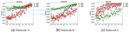
Figure 21.
Precision trend of weighted similarity indexes in different networks when increases.
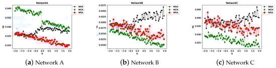
Figure 22.
RS trend of weighted similarity indexes in different networks when increases.
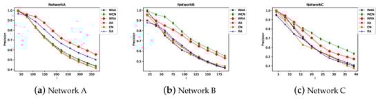
Figure 23.
Precision trend of the weighted and nonweighted similarity indexes when l increases and .
In summary, under optimal test-set-division conditions, the application of different similarity indexes to the commodity network obtained high prediction accuracy. The SRW index obtained the highest AUC of 0.97. The WRA and WCN indexes obtained marginally lower AUCs than the SRW index, achieving a value of 0.96; however, the algorithm time complexity of WRA and WCN indexes (, N is the count of node) is lower than that using the SRW index (, n is the steps, and k is average degree of network). More importantly, the precision is higher and RS is lower. Therefore, the WRA and WCN indexes are both suitable for commodity-related networks. The worst index is LHN-II, which obtained an AUC of only 0.5. Under the worse test-set-division condition, the AUC values of LRW-based similarity indexes were 0.8 and above, which shows that even if there are several missing edges in the network, a better prediction effect can be achieved. Each similarity index shows the following characteristics in the commodity network. (1) As the network edge information decreases, the prediction accuracy of the similarity index will gradually decrease. Therefore, in actual operations, the more complete the collected information is, the more beneficial it is to discover potentially related commodities. (2) When the network information is relatively complete, the prediction accuracy based on local network similarity indexes (such as LP, LRW, and SRW) is higher than that obtained by considering the global similarity indexes (such as Katz and ACT). However, if the network information is sparser, the accuracy is lower than that of the global indexes. When it is difficult to collect information, choosing a suitable global similarity measurement index can also obtain better prediction results. (3) In commodity networks transformed by association rules with different degrees of support, the prediction accuracy of each index is different. In Network A, the AUC was significantly higher. This also shows that when there are more nodes and edges in the network, the prediction effect will be better. (4) Effective use of weight information can improve prediction accuracy.
5.2. Potential Related Commodities
WRA was found to be an appropriate index. The details of the PRCD algorithm are shown in Algorithm 3, in which the input is transaction data, and the outputs are potential related commodities of each commodity in rules. Meanwhile, association rules are obtained by the apriori algorithm, and the commodity-related network is constructed based on them. In addition, the similarity between all goods without direct correlation is calculated, and for each good in the rules, the top N items with the highest similarity are found. refers to a vector including the similarity between commodity and other commodities that are not directly related. returns top N commodities set . Table 9 shows an example of 20 commodities with the highest similarity to the target commodity 21,086 (SET/6 RED SPOTTY PAPER CUPS) predicted in Network B. These commodities have a high probability of being potentially related to the target commodity.
Table 9.
Top 20 commodity sets with the highest similarity to the target commodity.
To verify whether there is an association relationship between two commodities whose predicted similarity is more than 0, the results of the three networks were tested. First, a lower support level of 0.001 was set to obtain the commodity-related Network D. Then, we checked whether the new connected edges (similarity more than 0) predicted in networks A, B, and C appeared in Network D. Finally, the ratios of the new connected edges that appear in Network D were calculated. For example, if there are 100 nonexisting edges with a similarity more than 0 in Network A, and 80 nonexisting edges of Network A appear in Network D, it implies that 80% of the predicted edges are actually weakly related.
The PRCD algorithm was executed in networks A, B, and C and returned similarity matrices , , and . The ratios of the new connected edges that were predicted to appear in Network D were calculated as 0.9695, 0.9995, and 1, respectively. This indicates that the predicted commodities with potential associations have a direct weak association relationship, and the proportion is very high, which shows that the algorithm to discover the potential association between commodities can identify the association relationship of the commodities outside the association rules. At the same time, it can also be proved that there is no competitive relationship between these commodities, because the probability of competing products appearing in the same basket is actually very small.
At the same time, in order to prove the practicality of the method, the PRCD was assessed on more common datasets of the recommendation system, which are shown in Table 10. Delicious contains social networking, bookmarking, and tagging information from a set of 2K users from the Delicious social bookmarking system. Lastfm corresponds to music artist listening information which was obtained from the Last.fm online music system. The BX dataset is a subset of the Book-Crossing dataset. The ML100K was collected through the MovieLens web site and each user has rated at least 20 movies. Similarly, the percent of the test set was set to 10%, and 10 times average AUC were obtained. The results show that the method still performs well in other datasets. Therefore, the method proposed can be used more widely.
Table 10.
The datasets used in evaluation.
5.3. Comparison to Other Methods
We conducted extensive experiments to evaluate PRCD. Our results show that PRCD achieves unprecedentedly strong performance on various datasets. In order to prove the superiority of the method, PRCD was compared with with link prediction methods based on graph neural networks (GNNs). SEAL permits learning from not only subgraph structures, but also latent and explicit node features, thus absorbing multiple types of information. It outperforms heuristic methods and latent feature methods. We used the same datasets as [] and ran all experiments for 10 times, then recorded the following average AUC results.
As shown in Table 11, the best result is bold. PRCD generally performs much better than traditional methods. This indicates that building an associated network before link prediction can improve the accuracy of prediction, especially the results on Router and Power. Meanwhile, SEAL shows better performance on NS, PB, Power, and Router. It can be seen that SEAL has outstanding learning ability for graphic features, but our method achieves comparable performances with SEAL. In addition, PRCD outperforms on USAir, Yeast, C. ele, and E. coil. In the real network, there will be some inessential and wrong links, which may affect the results that SEAL learns from the local subgraph. However, the main contribution of our proposed method lies in the construction of the network. By first obtaining interesting association rules and then building the network, some meaningless or unimportant links are eliminated in this process, which is beneficial to the training of algorithms and models.
Table 11.
Comparisons of average AUC of several methods.
6. Conclusions
This paper proposes a potentially related commodity discovery (PRCD) method based on link prediction. In this method, the association rules are used to construct the commodity association network in which the existing strong direct associations of commodities are considered. Meanwhile, the link prediction based on similarity is applied to the commodity association network. By comparing the influence of different similarity indexes on prediction accuracy, the most suitable similarity measurement indexes are found. The experimental results indicate that both WRA and WCN can effectively identify weak correlations between commodities and can predict the set of commodities with potential correlation with the target commodities. In addition, each index has different prediction accuracy in different commodity-related networks, thereby showing a certain regularity. The excellent performance of this method on other datasets proves the universality of this method.
The primary contributions of this paper are as follows: (1) A link prediction algorithm is applied to determine indirect association rules, which overcomes the lack of an important model owing to unreasonable support and confidence settings of association rules. Meanwhile, it can also reduce the screening of uninteresting association rules under low support. (2) The best similarity measurement indexes (WRA and WCN) are found, and in the commodity association networks, the utilization of lift and count as the weight can effectively improve the prediction accuracy of the algorithm. (3) This paper provides a new way to discover potential customers. By mining association rules, it can be determined that the target commodity A has a strong direct correlation with B. The customer of commodity B has a certain probability to become a potential customer of commodity A. Similarly, through the mining of potentially related commodities, it is possible to predict the set of commodities that have a potential relationship with the target commodity A, and then determine the potential customers of the commodity A.
The method has strong practical value. First, the method used in this paper does not have high requirements for data collection, and the collection cost is low. In addition, the time complexity of the algorithm is not high, practice is simple, and it is easy to popularize. Second, in actual use, it is possible to expand or reduce the collection of similar goods according to the actual requirements of each enterprise or merchant and control the scale of potentially related goods. Thirdly, the discovery of potentially related commodities results in accurate and timely predictions of customer requirements and improves service quality.
In the process of building a network, many nodes will inevitably be lost. This will lead to the problem of cold start. New products are often not added to the network as nodes. If the sup is set improperly, resulting in too few association rules, the prediction results will be inaccurate. If the sup is too small, the network structure may be too large. Determining how to set parameters according to different data needs further research.
Author Contributions
Conceptualization, H.L.; data curation, F.C.; formal analysis, X.W.; funding acquisition, H.L. and W.L.; investigation, X.W.; project administration, H.L.; resources, F.C.; software, X.W. and W.L.; supervision, X.W. and H.L.; validation, F.C. and H.L.; writing—original draft, F.C.; writing—review and editing, H.L. and F.C. All authors have read and agreed to the published version of the manuscript.
Funding
This work was supported by the National Natural Science Foundation of China (71771094).
Institutional Review Board Statement
Not applicable.
Informed Consent Statement
Not applicable.
Data Availability Statement
Not applicable.
Conflicts of Interest
The authors declare no conflict of interest. The funders had no role in the study design, data collection, analysis and interpretation, manuscript writing, or decision to publish the results.
References
- Kocas, C.; Pauwels, K.; Bohlmann, J.D. Pricing Best Sellers and Traffic Generators: The Role of Asymmetric Cross-selling. J. Interact. Mark. 2018, 41, 28–43. [Google Scholar] [CrossRef]
- Knott, A.; Hayes, A.; Neslin, S.A. Next-product-to-buy models for cross-selling applications. J. Interact. Mark. 2002, 16, 59–75. [Google Scholar] [CrossRef]
- Wong, C.W.; Fu, W.C.; Wang, K. Data Mining for Inventory Item Selection with Cross-Selling Considerations. Data Min. Knowl. Discov. 2005, 11, 81–112. [Google Scholar] [CrossRef][Green Version]
- Miswan, N.H.; Sulaiman, I.M.; Chan, C.S.; Ng, C.G. Association Rules Mining for Hospital Readmission: A Case Study. Mathematics 2021, 9, 2706. [Google Scholar] [CrossRef]
- Zhang, Z.; Huang, J.; Tan, Q. Association Rules Enhanced Knowledge Graph Attention Network. Knowl.-Based Syst. 2022, 239, 108038. [Google Scholar] [CrossRef]
- Telikani, A.; Gandomi, A.H.; Shahbahrami, A. A survey of evolutionary computation for association rule mining. Inf. Sci. 2020, 524, 318–352. [Google Scholar] [CrossRef]
- Liu, T.; Yin, X.; Ni, W. Next Basket Recommendation Model Based on Attribute-Aware Multi-Level Attention. IEEE Access 2020, 8, 153872–153880. [Google Scholar] [CrossRef]
- Chen, G.; Li, Z. A new method combining pattern prediction and preference prediction for next basket recommendation. Entropy 2021, 23, 1430. [Google Scholar] [CrossRef]
- AU Kim, J.K.; Moon, H.S.; An, B.J.; Choi, I.Y. A grocery recommendation for off-line shoppers. Online Inf. Rev. 2018, 42, 468–481. [Google Scholar] [CrossRef]
- Chen, Y.C.; Lee, G. An efficient projected database method for mining sequential association rules. In Proceedings of the 2010 Fifth International Conference on Digital Information Management (ICDIM), Thunder Bay, ON, Canada, 5–8 July 2010; IEEE: Piscataway, NJ, USA, 2010; pp. 274–278. [Google Scholar] [CrossRef]
- Liao, S.; Zou, T.; Chang, H. An Association Rules and Sequential Rules Based Recommendation System. In Proceedings of the 2008 4th International Conference on Wireless Communications, Networking and Mobile Computing, Dalian, China, 12–17 October 2008; IEEE: Piscataway, NJ, USA, 2008; pp. 1–4. [Google Scholar] [CrossRef]
- Lü, L.; Zhou, T. Link prediction in complex networks: A survey. Phys. Stat. Mech. Its Appl. 2011, 390, 1150–1170. [Google Scholar] [CrossRef]
- Biondi, G.; Franzoni, V. Discovering Correlation Indices for Link Prediction Using Differential Evolution. Mathematics 2020, 8, 2097. [Google Scholar] [CrossRef]
- Sarukkai, R.R. Link prediction and path analysis using Markov chains. Comput. Netw. 2000, 33, 377–386. [Google Scholar] [CrossRef]
- Yadav, R.; Rai, A. Incorporating communities’ structures in predictions of missing links. J. Intell. Inf. Syst. 2020, 55, 183–205. [Google Scholar] [CrossRef]
- Wang, G.; Wang, Y.; Li, J.; Liu, K. A multidimensional network link prediction algorithm and its application for predicting social relationships. J. Comput. Sci. 2021, 53, 101358. [Google Scholar] [CrossRef]
- Kumar, M.; Mishra, S.; Biswas, B. Features fusion based link prediction in dynamic neworks. J. Comput. Sci. 2022, 57, 101493. [Google Scholar] [CrossRef]
- Liu, J.; Xu, B.; Xu, X.; Xin, T. A link prediction algorithm based on label propagation. J. Comput. Sci. 2016, 16, 43–50. [Google Scholar] [CrossRef]
- Sharma, U.; Kandwal, S.; Khatri, S.K. A Link Prediction in Social Networks: A Fuzzy Cognitive Map Approach. In Ambient Communications and Computer Systems; Springer: Singapore, 2018; pp. 463–473. [Google Scholar] [CrossRef]
- Li, S.; Song, X.; Lu, H.; Zeng, L.; Shi, M.; Liu, F. Friend recommendation for cross marketing in online brand community based on intelligent attention allocation link prediction algorithm. Expert Syst. Appl. 2019, 139, 112839. [Google Scholar] [CrossRef]
- Kovács, I.A.; Luck, K.; Spirohn, K.; Wang, Y.; Pollis, C.; Schlabach, S.; Bian, W.; Kim, D.K.; Kishore, N.; Hao, T.; et al. Network-based prediction of protein interactions. Nat. Commun. 2019, 10, 1240. [Google Scholar] [CrossRef]
- Zhang, F.; Qi, S.; Liu, Q.; Mao, M.; Zeng, A. Alleviating the data sparsity problem of recommender systems by clustering nodes in bipartite networks. Expert Syst. Appl. 2020, 149, 113346. [Google Scholar] [CrossRef]
- Li, C.; Yang, Q.; Pang, B.; Chen, T.; Cheng, Q.; Liu, J. A Mixed Strategy of Higher-Order Structure for Link Prediction Problem on Bipartite Graphs. Mathematics 2021, 9, 3195. [Google Scholar] [CrossRef]
- Gharibshah, J.; Jalili, M. Connectedness of users–items networks and recommender systems. Appl. Math. Comput. 2014, 243, 578–584. [Google Scholar] [CrossRef]
- Lee, Y.L.; Zhou, T. Collaborative filtering approach to link prediction. Phys. Stat. Mech. Its Appl. 2021, 578, 126107. [Google Scholar] [CrossRef]
- Coscia, M.; Szell, M. Multiplex Graph Association Rules for Link Prediction. arXiv 2020, arXiv:2008.08351. [Google Scholar] [CrossRef]
- Kardan, A.A.; Ebrahimi, M. A novel approach to hybrid recommendation systems based on association rules mining for content recommendation in asynchronous discussion groups. Inf. Sci. 2013, 219, 93–110. [Google Scholar] [CrossRef]
- Ekstrand, M.D.; Riedl, J.T.; Konstan, J.A. Collaborative Filtering Recommender Systems. Found. Trends Hum.–Comput. Interact. 2011, 4, 81–173. [Google Scholar] [CrossRef]
- Lu, Q.; Guo, F. Personalized information recommendation model based on context contribution and item correlation. Measurement 2019, 142, 30–39. [Google Scholar] [CrossRef]
- Vinodhini, G.; Chandrasekaran, R.M. Measuring the quality of hybrid opinion mining model for e-commerce application. Measurement 2014, 55, 101–109. [Google Scholar] [CrossRef]
- Yi, S.; Liu, X. Machine learning based customer sentiment analysis for recommending shoppers, shops based on customers’review. Complex Intell. Syst. 2020, 6, 621–634. [Google Scholar] [CrossRef]
- Bobadilla, J.; Ortega, F.; Hernando, A.; Gutiérrez, A. Recommender systems survey. Knowl.-Based Syst. 2013, 46, 109–132. [Google Scholar] [CrossRef]
- Nilashi, M.; Ibrahim, O.; Bagherifard, K. A recommender system based on collaborative filtering using ontology and dimensionality reduction techniques. Expert Syst. Appl. 2018, 92, 507–520. [Google Scholar] [CrossRef]
- Yang, D.; Nie, Z.T.; Yang, F. Time-Aware CF and Temporal Association Rule-Based Personalized Hybrid Recommender System. J. Organ. End User Comput. 2021, 33, 19–34. [Google Scholar] [CrossRef]
- Li, H. Time works well: Dynamic time warping based on time weighting for time series data mining. Inf. Sci. 2021, 547, 592–608. [Google Scholar] [CrossRef]
- Esling, P.; Agon, C. Time-Series Data Mining. ACM Comput. Surv. 2012, 45, 1–34. [Google Scholar] [CrossRef]
- Li, H.; Liu, Z. Multivariate time series clustering based on complex network. Pattern Recognit. 2021, 115, 107919. [Google Scholar] [CrossRef]
- Lin, W.; Wu, X.; Wang, Z.; Wan, X.; Li, H. Topic Network Analysis Based on Co-Occurrence Time Series Clustering. Mathematics 2022, 10, 2846. [Google Scholar] [CrossRef]
- Li, H.; Wu, Y.J.; Chen, Y. Time is money: Dynamic-model-based time series data-mining for correlation analysis of commodity sales. J. Comput. Appl. Math. 2020, 370, 112659. [Google Scholar] [CrossRef]
- Chen, Z.; Fan, Z.; Sun, M. A multi-kernel support tensor machine for classification with multitype multiway data and an application to cross-selling recommendations. Eur. J. Oper. Res. 2016, 255, 110–120. [Google Scholar] [CrossRef]
- Mazeh, I.; Shmueli, E. A personal data store approach for recommender systems: Enhancing privacy without sacrificing accuracy. Expert Syst. Appl. 2020, 139, 112858. [Google Scholar] [CrossRef]
- Wang, C.; Zheng, Y.; Jiang, J.; Ren, K. Toward Privacy-Preserving Personalized Recommendation Services. Engineering 2018, 4, 21–28. [Google Scholar] [CrossRef]
- Hurley, N.; Zhang, M. Novelty and Diversity in top-N recommendation-Analysis and evaluation. ACM Trans. Internet Technol. 2010, 10, 14-1–14-30. [Google Scholar] [CrossRef]
- Wang, F.; Wen, Y.; Wu, R.; Liu, J.; Cao, B. Improving the novelty of retail commodity recommendations using multiarmed bandit and gradient boosting decision tree. Concurr. Comput. Pract. Exp. 2020, 32, e5703. [Google Scholar] [CrossRef]
- Xia, H.; Huang, K.; Liu, Y. Unexpected interest recommender system with graph neural network. Complex Intell. Syst. 2022. [Google Scholar] [CrossRef]
- Ghafari, S.M.; Tjortjis, C. A survey on association rules mining using heuristics. WIREs Data Min. Knowl. Discov. 2019, 9, e1307. [Google Scholar] [CrossRef]
- Han, X.; Jiang, F.; Needleman, J.; Zhou, H.; Yao, C.; lang Tang, Y. Comorbidity combinations in schizophrenia inpatients and their associations with service utilization: A medical record-based analysis using association rule mining. Asian J. Psychiatry 2022, 67, 102927. [Google Scholar] [CrossRef]
- Gakii, C.; Rimiru, R. Identification of cancer related genes using feature selection and association rule mining. Inform. Med. Unlocked 2021, 24, 100595. [Google Scholar] [CrossRef]
- Zai-Xiang, H.; Zhong-Mei, Z.; Tian-Zhong, H.; Yi-Feng, Z. Improved associative classification algorithm for multiclass imbalanced datasets. Pattern Recognit. Artif. Intell. 2015, 28, 922–929. [Google Scholar] [CrossRef]
- Liu, J.; Shi, D.; Li, G.; Xie, Y.; Li, K.; Liu, B.; Ru, Z. Data-driven and association rule mining-based fault diagnosis and action mechanism analysis for building chillers. Energy Build. 2020, 216, 109957. [Google Scholar] [CrossRef]
- Bohmer, K.; Rinderle-Ma, S. Mining association rules for anomaly detection in dynamic process runtime behavior and explaining the root cause to users. Inf. Syst. 2020, 90, 101438. [Google Scholar] [CrossRef]
- Zhou, Y.; Li, C.; Ding, L.; Sekula, P.; Love, P.E.; Zhou, C. Combining association rules mining with complex networks to monitor coupled risks. Reliab. Eng. Syst. Saf. 2019, 186, 194–208. [Google Scholar] [CrossRef]
- Agrawal, R.; Imieliński, T.; Swami, A. Mining Association Rules Between Sets of Items in Large Databases. ACM Sigmod Rec. 1993, 22, 207–216. [Google Scholar] [CrossRef]
- Han, J.; Jian, P.; Yin, Y.; Mao, R. Mining Frequent Patterns without Candidate Generation: A Frequent-Pattern Tree Approach. Data Min. Knowl. Discov. 2004, 8, 53–87. [Google Scholar] [CrossRef]
- Cózar, J.; delaOssa, L.; Gámez, J. Learning compact zero-order TSK fuzzy rule-based systems for high-dimensional problems using an Apriori + local search approach. Inf. Sci. 2018, 433, 1–16. [Google Scholar] [CrossRef]
- Baró, G.; Martĺnez-Trinidad, J.; Rosas, R.; Ochoa, J.; Cortés, M. A PSO-based algorithm for mining association rules using a guided exploration strategy. Pattern Recognit. Lett. 2020, 138, 8–15. [Google Scholar] [CrossRef]
- Tan, P.N.; Kumar, V.; Srivastava1, J. Indirect Association: Mining Higher Order Dependencies in Data. In Principles of Data Mining and Knowledge Discovery; Springer: Berlin/Heidelberg, Germany, 2000; pp. 632–637. [Google Scholar] [CrossRef]
- Wan, Q.; An, A. An efficient approach to mining indirect associations. J. Intell. Inf. Syst. 2006, 27, 135–158. [Google Scholar] [CrossRef]
- Ouyang, W.; Luo, S.; Huang, Q.; CIS. Discovery of Direct and Indirect Association Patterns in Large Transaction Databases. In Proceedings of the Computational Intelligence and Security (CIS), 2007 International Conference, Harbin, China, 15–19 December 2007; IEEE: Piscataway, NJ, USA, 2007; pp. 167–170. [Google Scholar] [CrossRef]
- Tan, P.N.; Kumar, V. Discovery of Indirect Associations from Web Usage Data. In Web Intelligence; Springer: Berlin/Heidelberg, Germany, 2003; pp. 128–152. [Google Scholar] [CrossRef]
- Kazienko, P. Product Recommendation in e-Commerce Using Direct and Indirect Confidence for Historical User Sessions. In Discovery Science; Suzuki, E., Arikawa, S., Eds.; Springer: Berlin/Heidelberg, Germany, 2004; pp. 255–269. [Google Scholar] [CrossRef]
- Zhang, M.; Chen, Y. Link Prediction Based on Graph Neural Networks. In Proceedings of the 32nd International Conference on Neural Information Processing Systems, Montreal, QC, Canada, 3–8 December 2018; Curran Associates Inc.: Sydney, Australia, 2018; pp. 5171–5181. [Google Scholar] [CrossRef]
- Ye, X.; Rockmore, D.; Kleinbaum, A.M. Hyperlink Prediction in Hypernetworks Using Latent Social Features. In Proceedings of the International Conference on Discovery Science, Singapore, 6–9 October 2013. [Google Scholar] [CrossRef]
- Zhang, M.; Cui, Z.; Jiang, S.; Chen, Y. Beyond Link Prediction: Predicting Hyperlinks in Adjacency Space. In Proceedings of the Association for the Advancement of Artificial Intelligence, New Orleans, LA, USA, 2–7 February 2018. [Google Scholar]
- Pan, L.; Shang, H.J.; Li, P.; Dai, H.; Wang, W.; Tian, L. Predicting hyperlinks via hypernetwork loop structure. EPL 2021, 135, 48005. [Google Scholar] [CrossRef]
- Xiao, G.; Liao, J.; Tan, Z.; Zhang, X.; Zhao, X. A Two-Stage Framework for Directed Hypergraph Link Prediction. Mathematics 2022, 10, 2372. [Google Scholar] [CrossRef]
- Leicht, E.; Holme, P.; Newman, M. Vertex similarity in networks. Phys. Rev. E 2006, 73, 026120. [Google Scholar] [CrossRef] [PubMed]
- Ravasz, E.; Somera, A.L.; Mongru, D.A.; Oltvai, Z.N.; Barabási, A.L. Hierarchical organization of modularity in metabolic networks. Science 2002, 297, 1551–1555. [Google Scholar] [CrossRef] [PubMed]
- Jaccard, P. Etude comparative de la distribution florale dans une portion des Alpes et des Jura. Bull. SociéTé Vaudoise Des Sci. Nat. 1901, 37, 547–579. [Google Scholar] [CrossRef]
- Barabási, A.L.; Albert, R. Emergence of scaling in random networks. Science 1999, 286, 509–512. [Google Scholar] [CrossRef]
- Adamic, L.; Adar, E. Friends and neighbors on the Web. Soc. Netw. 2003, 25, 211–230. [Google Scholar] [CrossRef]
- Zhou, T.; Lü, L.; Zhang, Y.C. Predicting missing links via local information. Eur. Phys. J. B 2009, 71, 623–630. [Google Scholar] [CrossRef]
- Lü, L.; Jin, C.H.; Zhou, T. Similarity index based on local paths for link prediction of complex networks. Phys. Rev. E 2009, 80, 046122. [Google Scholar] [CrossRef] [PubMed]
- Katz, L. A new status index derived from sociometric analysis. Psychometrika 1953, 18, 39–43. [Google Scholar] [CrossRef]
- Klein, D.; Randić, M. Resistance distance. J. Math. Chem. 1993, 12, 81–95. [Google Scholar] [CrossRef]
- Fouss, F.; Pirotte, A.; Renders, J.M.; Saerens, M. Random-walk computation of similarities between nodes of a graph with application to collaborative recommendation. IEEE Trans. Knowl. Data Eng. 2007, 19, 355–369. [Google Scholar] [CrossRef]
- Brin, S.; Page, L. The anatomy of a large-scale hypertextual Web search engine. Comput. Netw. 2012, 56, 3825–3833. [Google Scholar] [CrossRef]
- Jeh, G.; Widom, J. SimRank: A measure of structural-context similarity. In Proceedings of the 8th ACM(Association for Computing Machinery) SIGKDD(Special Interest Group on Knowledge Discovery and Data Mining) International Conference on Knowledge Discovery and Data Mining, Edmonton, AB, Canada, 23–26 July 2002; pp. 538–543. [Google Scholar] [CrossRef]
- Liu, W.; Lü, L. Link prediction based on local random walk. Europhys. Lett. 2010, 89, 58007. [Google Scholar] [CrossRef]
- Lü, L.; Zhou, T. Link prediction in weighted networks: The role of weak ties. Europhys. Lett. 2010, 89, 18001. [Google Scholar] [CrossRef]
Publisher’s Note: MDPI stays neutral with regard to jurisdictional claims in published maps and institutional affiliations. |
© 2022 by the authors. Licensee MDPI, Basel, Switzerland. This article is an open access article distributed under the terms and conditions of the Creative Commons Attribution (CC BY) license (https://creativecommons.org/licenses/by/4.0/).