Optimization Methods for Redundancy Allocation in Hybrid Structure Large Binary Systems

Abstract

This paper addresses the issue of optimal redundancy allocation in hybrid structure large binary systems. Two aspects of optimization are considered: (1) maximizing the reliability of the system under the cost constraint, and (2) obtaining the necessary reliability at a minimum cost. The complex binary system considered in this work is composed of many subsystems with redundant structure. To cover most of the cases encountered in practice, the following kinds of redundancy are considered: active redundancy, passive redundancy, hybrid standby redundancy with a hot or warm reserve and possibly other cold ones, triple modular redundancy (TMR) structure with control facilities and cold spare components, static redundancy: triple modular redundancy or 5-modular redundancy (5MR), TMR/Simplex with cold standby redundancy, and TMR/Duplex with cold standby redundancy. A classic evolutionary algorithm highlights the complexity of this optimization problem. To master the complexity of this problem, two fundamentally different optimization methods are proposed: an improved evolutionary algorithm and a zero-one integer programming formulation. To speed up the search process, a lower bound is determined first. The paper highlights the difficulty of these optimization problems for large systems and, based on numerical results, shows the effectiveness of zero-one integer programming.

1. Introduction

The problem of reliability optimization in large hybrid systems mainly refers to the type of the system (binary or multi-state), type of solution (reliability allocation and/or redundancy allocation), or the kind of redundancy, which can be static (TMR or 5MR, for example), dynamic (active redundancy or standby redundancy), or hybrid (TMR/Simplex or TMR/Duplex with spare components, etc.). Useful overviews covering models and methods for these reliability optimization problems (ROPs), including reliability allocation, redundancy allocation, and reliability-redundancy allocation can be found in many works, such as [1,2,3].

The mathematical formulation of a reliability optimization problem requires the specification of three elements: decision variables, imposed constraints, and objective function(s).

The decision variables describe those elements that can be changed or adjusted or the decisions that can be made to improve system performance, as expressed by the objective function(s). As examples of decision variables one can mention the types of components and their characteristics (reliability, cost, etc.), the type of redundancy for each subsystem, the number of spare components for each subsystem, etc.

The constraints reflect practical design limitations, e.g., a required level of reliability or the available budget, which occur in almost all cases. But in practice there may be other limitations, related to the volume or weight of the system, for example.

The objective function measures the performance of the system for a set of values of the decision variables. Thus, by optimizing the objective function(s) under the specified constraints it is possible to identify the combination of values of the decision variables that leads to the best possible design solution for the studied system.

Usually for ROPs, the goal of optimization is to maximize system reliability or minimize system cost. In reliability engineering the problem of system reliability maximization under two or more constraints often arises, e.g., under cost constraints, but also under weight and/or volume constraints. When an analytical approach is possible (e.g., in the case of active-redundancy-only subsystems), to ensure that two or more constraints are satisfied, Lagrangian multipliers are often introduced as part of the objective function [4,5,6].

In this paper we address a class of redundancy allocation problems (RAPs) where the decision variable is the number of redundant components for each subsystem in a series redundant reliability model. RAP is one of the most studied reliability optimization problems, because it has been proven to be quite difficult to solve, and many different optimization approaches have been used to determine optimal or near-optimal solutions. As [7] demonstrates, RAPs belong to the NP-hard class of optimization problems.

The RAPs we consider involves hybrid structures with no less than eight types of redundancy; these are conditions where the optimization problems are difficult to solve, even if we limit ourselves to single-constraint optimization problems. More specifically, our goal is to highlight the difficulty of these RAPs for large systems, when the number of subsystems grows to the order of tens or even hundreds.

In order to master the complexity of RAPs in case of large systems, for which the difficulty of the problem increases, special research efforts have been made in recent years. In addition, to cover a wide range of techniques used to increase the reliability encountered in practice, many hybrid reliability models have been considered for which the RAPs get even more complicated. For example, [8] investigates a complex reliability-redundancy allocation problem with a component mixing strategy, which changes the traditional RAP model to a heterogeneous one. Moreover, in the hybrid reliability models proposed in [9], the choice of redundancy strategy is considered as a decision variable. So, for each subsystem, an active or cold standby redundancy may be considered. In addition, components of different types can be used in each subsystem, i.e., a component mixing strategy. Consequently, this RAP involves determining a solution that maximizes system reliability in terms of the type of redundancy and the number of spare components of each type (for each subsystem). To solve this RAP, a genetic algorithm is developed. Also, a reliability model based on cold standby redundancy combined with component mixing is investigated by [10]. For this complex problem, the author proposes a simplified swarm optimization method in which a multi-role resource sharing strategy is adopted to provide the diverse system components. Another reliability model based on active or cold standby redundancy combined with component mixing is investigated in [11]. To solve this RAP, the authors propose a parallel stochastic fractal search algorithm. Other RAPs involving a heterogeneous structure and/or component allocation strategy of a different type can be found in [12,13,14].

Such a hybrid reliability model is also considered in this paper. In the previously cited works, RAPs are formulated by considering redundant systems with hybrid redundancy strategies and/or reliability models with heterogeneous components, which means that each component of a subsystem can have its own failure rate. In this paper we limit ourselves to the case where subsystems include homogeneous components, but we extend RAPs to cover more redundancy strategies (not just active redundancy or cold standby), including static redundancy or reconfigurable structures such as TMR/Simplex or TMR/Duplex with cold standby redundancy.

To solve redundancy allocation problems of this type, several techniques can be applied, such as heuristic methods [15,16,17,18], Lagrange multiplier analytical methods, and branch-and-bound techniques, especially for active redundancy [5,6,19,20], dynamic programming [21,22,23], evolutionary algorithms [9,10,24,25,26,27], linear programming methods [28,29,30] or a mix of integer and nonlinear programming [31]. As the RAPs we considered are complex, two evolutionary algorithms and a special model of zero-one integer programming are used.

As the highlights of our contribution we can mention:

• The formalization of two RAPs for binary systems with hybrid structure, which include no less than eight types of redundancy, where reliability modeling of redundant and reconfigurable structures is based on Markov chains;
• The design and implementation of two evolutionary algorithms and the formulation of a zero-one integer program for solving these complex optimization problems;
• Conducting an extensive performance evaluation study of the three proposed techniques on thousands of problems, which demonstrates the effectiveness of the zero-one integer programming approach for large systems with tens or even hundreds of subsystems.

This paper is organized as follows. Section 2 presents the issue addressed, whereas the types of redundancy considered here and the models or equations used for reliability evaluation are presented in detail in Section 3. Some related works are mentioned in Section 4. The algorithms used for these optimal allocation issues are described in Section 5. The objective functions adopted for the evolutionary algorithms and for the linear programming model are reported in Section 6, whereas in Section 7 a lower bound solution is proven. Experimental results are presented in Section 8. Further discussion is the subject of Section 9. The conclusions of the paper and several directions of future research are included in Section 10.

2. Problem Description

For systems with a large number of components without redundancy, reliability is often very low. To achieve the required reliability, a certain type of redundancy is applied to a certain element, depending on technical particularities, which can be static, dynamic, or hybrid redundancy. All of these types of redundancy are considered in this paper. The reliability model for this redundant system is a series-redundant one as presented in Figure 1.

The notations used to describe the redundant structures and their reliability evaluation models are presented at the end of the paper. Along with these notations we include a short nomenclature and some assumptions under which the reliability models are valid.

Typically, in this allocation process the criterion may be reliability, cost, weight, or volume. One or more criteria can be considered in an objective function, while the others may be considered constraints, as considered by [22] (pp. 331–338). In this paper, the criteria we consider are reliability and cost, and in this situation, two optimization problems are frequently encountered in practice:

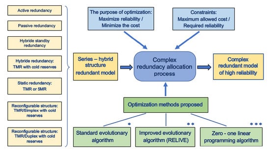
• Minimizing the cost of the redundant system for which a required reliability must be achieved;
• Maximizing the reliability of the system within a maximum allowed cost.

In both cases, from the mathematical point of view, one must solve an optimization problem with an objective function and constrains. More exactly, for the first problem, one must minimize the cost function:

$$C_{rs}=f\left(C_1, C_2, \cdots ,C_n\right)={\displaystyle \sum }_{i=1}^n{C}_i$$

(1)

with the constraint of reliability:

$$R_{rs}={\displaystyle \prod }_{i=1}^n{R}_i\ge R^{*}.$$

(2)

For the second problem, one must maximize the reliability function:

$$R_{rs}=f\left(R_1, R_2, \cdots ,R_n\right)={\displaystyle \prod }_{i=1}^n{R}_i$$

(3)

with the cost constraint:

$${\displaystyle \sum }_{i=1}^n{C}_i\le C^{*}.$$

(4)

For example, when for all the subsystems an active redundancy is considered, for the redundant system a series-parallel reliability model results. Thus, the cost and reliability functions can be expressed by the equations:

$$C_{rs}={\displaystyle \sum }_{i=1}^n{c}_i{k}_i$$

(5)

$$R_{rs}=1-{\displaystyle \prod }_{i=1}^n{\left(1-r_i\right)}^{k_i}$$

(6)

Thus, we have to determine the values $k_1$, $k_2$, …, $k_n$ that minimize the cost function in Equation (5) with the reliability constraint in Equation (2), or maximize the reliability function in Equation (6) with the cost constraint in Equation (4), as the case may be.

3. Types of Redundancy

To cover most situations encountered in practice, the following types of redundancy are considered in this study, namely:

• active redundancy $\left(tr=\mathrm{A}\right)$;
• passive redundancy (or cold standby redundancy) $\left(tr=\mathrm{B}\right)$;
• hybrid standby redundancy with a hot reserve $\left(tr=\mathrm{C}\right)$ or a warm one $\left(tr=\mathrm{D}\right)$ and possibly other cold ones;
• hybrid redundancy consisting of a TMR structure with control facilities and possibly cold reserves $\left(tr=\mathrm{E}\right);$
• static redundancy: TMR or 5MR $\left(tr=\mathrm{F}\right);$
• reconfigurable TMR/Simplex type structure with possible other cold-maintained spare components $\left(tr=\mathrm{G}\right)$;
• reconfigurable TMR/Duplex type structure with possible other cold-maintained spare components $\left(tr=\mathrm{H}\right).$

The reliability model and the equations used to evaluate the reliability for a subsystem, depending on the type of redundancy, are presented in this section. Since the time to failure for a component is assumed to have a negative exponential distribution, the following equations are valid:

$$r=e^{-\lambda T}$$

(7)

and

$$\lambda T=-\ln r$$

(8)

Remember that for any redundant subsystem the spare components are considered identical to the basic ones.

3.1. Active Redundancy ($tr=A$)

For this parallel reliability model where all components operate simultaneously, the well-known equation is applied:

$$R=1-{\left(1-r\right)}^k, k=2, 3, \dots$$

(9)

3.2. Passive Redundancy ($tr=B$)

In this case, one component is in operation and all other identical $k-1$ spare components are maintained in a cold state, which means that a spare component is switched off until it is needed to replace the defective one (i.e., a redundant component does not fail in cold standby mode). The following equation can be applied to this model:

$$R={\displaystyle \sum }_{j=0}^{k-1}\frac{{\left(\lambda T\right)}^j}{j!}{e}^{-\lambda T}=r{\displaystyle \sum }_{j=0}^{k-1}\frac{{\left(-\ln r\right)}^j}{j!}, k\ge 2$$

(10)

Note that Equation (10) is the sum of the first $k$ terms of the Poisson distribution of the parameter $\lambda T$.

3.3. Hybrid Standby Redundancy with a Hot ($tr=C$) or a Warm ($tr=D$) Spare and Possibly Other Cold Ones

In this case of standby redundancy, a component is in operation, a spare component is active or kept in a warm state, and possibly other spare components are kept in cold conditions as illustrated in Figure 2.

A warm component may fail before being put into operation and its failure rate is less than that of the same component in active mode. Therefore, let $\alpha \lambda , 0<\alpha \le 1$, be the failure rate for this reserve. For this type of redundancy, the subsystem reliability function is obtained based on the Markov method, depending on the total number of components, as shown below.

3.3.1. Case 1: $k=2$

Consider a subsystem consisting of a component in operation and a warm-maintained reserve. The evolution of this redundant subsystem until failure is illustrated by the Markov chain presented in Figure 3.

To begin with, let us refer to a general Markov model. Let $S_1, S_2, \dots , S_N$ be the states of the Markov chain and $A={\left[a_{x,y}\right]}_{N\times N}$ be the matrix of state transition rates, where $a_{x,y}, x\ne y$, represents the rate of transition from state $S_y$ to state $S_x$, while an element of the main diagonal (i.e., $x=y$) is the negative value of the sum of all the other elements in the column.

Let $s\left(t\right)$ be the state of the subsystem at the time $t$, and

$$p_x\left(t\right)=\mathrm{prob}\left(s\left(t\right)=S_x\right), x\in \left\{1, 2, \dots , N\right\}.$$

(11)

To obtain the probability functions $p_x\left(t\right), x=1:N,$ the following system of differential equations must be solved:

$$P^{\prime }=A\times P,$$

(12)

where $P= {\left[p_1\left(t\right) p_2\left(t\right) \cdots p_N\left(t\right)\right]}^T,$ and $P^{\prime }={\left[p_1^{\prime }\left(t\right) p_2^{\prime }\left(t\right) \cdots p_N^{\prime }\left(t\right)\right]}^T$.

Note that the state probabilities for $t=0$ are also known.

Let us resume the analysis of the subsystem under study. In the Markov chain presented in Figure 3, $S_1$ and $S_2$ are successful states, while $S_3$ is a failure state. Thus, the reliability function of this redundant subsystem can be defined as

$$R\left(t\right)=p_1\left(t\right)+p_2\left(t\right), t\ge 0.$$

(13)

As the transition rate matrix is:

$$A=\left[\begin{array}{ccc}-\left(1+\alpha \right)\lambda & 0& 0\\ \left(1+\alpha \right)\lambda & -\lambda & 0\\ 0& \lambda & 0\end{array} \right],$$

(14)

to determine the probability functions $p_1\left(t\right)$ and $p_2\left(t\right)$, the following system of differential equations must be solved:

$$\{\begin{array}{l}{p}_1^{\prime }\left(t\right)=-\left(1+\alpha \right)\lambda p_1\left(t\right)\hfill \\ p_2^{\prime }\left(t\right)=\left(1+\alpha \right)\lambda p_1\left(t\right)-\lambda p_2\left(t\right)\hfill \end{array}$$

(15)

With the initial values: $p_1\left(0\right)=1 \mathrm{and} p_2\left(0\right)=p_3\left(0\right)=0$, by applying the Laplace transform ($ℒ$), the following system of algebraic equations results:

$$\{ \begin{array}{l}s{P}_1\left(s\right)-1=-\left(1+\alpha \right)\lambda P_1\left(s\right)\hfill \\ s{P}_2\left(s\right)=\left(1+\alpha \right)\lambda P_1\left(s\right)-\lambda P_2\left(s\right)\hfill \end{array}$$

(16)

where $P_i\left(s\right)=ℒ \left\{p_i\left(t\right)\right\}, i\in \left\{1, 2\right\}$, are functions in the frequency domain, and $s$ is the Laplace operator. Based on (16), after some algebraic operations, the following functions are obtained:

$$P_1\left(s\right)=\frac{1}{s+\left(1+\alpha \right)\lambda }, P_2\left(s\right)=\frac{\left(1+\alpha \right)\lambda }{s+\left(1+\alpha \right)\lambda }·\frac{1}{s+\lambda }$$

(17)

After a partial-fraction-expansion, the function $P_2\left(s\right)$ can be expressed as follows:

$$P_2\left(s\right)=-\frac{1+\alpha }{\alpha }\frac{1}{s+\left(1+\alpha \right)\lambda }+\frac{1+\alpha }{\alpha }\frac{1}{s+\lambda }$$

(18)

As the function $\mathcal{R}\left(s\right)=ℒ\left\{R\left(t\right)\right\}=P_1\left(s\right)+P_2\left(s\right),$ the following expression results:

$$\mathcal{R}\left(s\right)=\frac{1+\alpha }{\alpha }\frac{1}{s+\lambda }-\frac{1}{\alpha }\frac{1}{s+\left(1+\alpha \right)\lambda }$$

(19)

The reliability function $R\left(t\right)$ can then be obtained by applying the inverse Laplace transform, $R\left(t\right)={ℒ}^{-1}\left\{\mathcal{R}\left(s\right)\right\}$. Thus, the reliability function has the following form:

$$R\left(t\right)=\frac{1+\alpha }{\alpha }{e}^{-\lambda t}-\frac{1}{\alpha }{e}^{-\left(1+\alpha \right)\lambda t}, t\ge 0, 0<\alpha \le 1.$$

(20)

For a certain period of time $T$, the component reliability is $r=e^{-\lambda T},$ so that the subsystem reliability R as a function of r and $\alpha$ is given by the equation:

$$R\left(r, \alpha \right)=\frac{1+\alpha }{\alpha }r-\frac{1}{\alpha }{r}^{1+\alpha }=r+\frac{1}{\alpha }r\left(1-r^{\alpha }\right), 0<\alpha \le 1.$$

(21)

For a redundancy subsystem with a larger number of components, the reliability function can be obtained based on the Markov method in the same way, but algebraic operations are more complicated. The results for the other two cases are presented below.

3.3.2. Case 2: $k=3$

Take a redundant subsystem composed of an active component, a hot/warm spare component, and another one maintained in cold conditions. For this case, the following reliability function results:

$$R\left(r, \alpha \right)=\frac{{\left(1+\alpha \right)}^2}{{\alpha }^2}r-\left(\frac{1+2\alpha }{{\alpha }^2}-\frac{1+\alpha }{\alpha }\ln r\right)r^{1+\alpha }, 0<\alpha \le 1.$$

(22)

3.3.3. Case 3: $k=4$

For a redundant subsystem with an active component, a hot/warm spare component, and two other ones maintained in cold conditions, the reliability function is given by the following equation:

$$R\left(r, \alpha \right)=\frac{{\left(1+\alpha \right)}^3}{{\alpha }^3}r-\left(\frac{1+3\alpha +3{\alpha }^2}{{\alpha }^3}-\frac{1+3\alpha +2{\alpha }^2}{{\alpha }^2}\ln r+\frac{{\left(1+\alpha \right)}^2}{2\alpha }{\left(\ln r\right)}^2\right)r^{1+\alpha }, 0<\alpha \le 1.$$

(23)

3.4. TMR Structure with Control Facilities and Cold Spare Components ($tr=E$)

In this case, another hybrid redundancy is considered. Thus, a redundant system is composed of a TMR structure with control facilities as a basic structure (i.e., static redundancy) and possibly one or more components maintained in cold conditions (i.e., standby redundancy). This type a hybrid redundancy is illustrated in Figure 4.

The decision logic works on the principle of majority logic, 2 out of 3, called $\mathrm{voter}$ and represented by the symbol V in Figure 4. When one of the three components in operation (${\mathrm{CO}}_1$, ${\mathrm{CO}}_2$ or ${\mathrm{CO}}_3)$ fails, an error signal indicates the faulty component. Thus, the faulty component can be replaced with a cold-maintained standby one as soon as possible. In this way, this redundant hybrid subsystem can tolerate one or more defective components, as the case may be. For additional decision and control block the failure rate, denoted by ${\lambda }_{dc}$, is expressed based on the basic component rate, $\lambda$. In this study, the following expression is used:

$${\lambda }_{dc}=\frac{\lambda }{\beta }, \beta >1.$$

(24)

Consequently, the reliability function for logical decision and control block, denoted by $r_{dc}$, is expressed as:

$$r_{dc}=e^{-{\lambda }_{dc}T}=e^{-\frac{\lambda }{\beta } T}={\left(e^{-\lambda T}\right)}^{{\beta }^{-1}}=r^{{\beta }^{-1}}, \beta >1.$$

(25)

3.4.1. Case 1: TMR Structure without Standby Redundancy

In case of a TMR structure without reserves (i.e., $k=3$), the redundant subsystem can tolerate only one faulty component, so the subsystem reliability function is given by the well-known equation:

$$R\left(r, \beta \right)=\left(3r^2-2r^3\right)r_{dc}=\left(3r^2-2r^3\right)r^{{\beta }^{-1}}, \beta >1$$

(26)

3.4.2. Case 2: TMR Structure and One Cold Spare Component

A redundant subsystem with hybrid redundancy composed of a TMR structure and one CSC (i.e., $k=4$) may tolerate two faulty components. For a start, for the logical block of decision and control, the possibility of failure is neglected. The reliability evaluation is made based on the Markov graph given in Figure 5.

In this graph, $S_1, S_2$ and $S_3$ are successful states, while $S_4$ is a failure one. Given these aspects, the reliability function of this redundant subsystem is expressed as:

$$R\left(t\right)=p_1\left(t\right)+p_2\left(t\right)+p_3\left(t\right), t\ge 0.$$

(27)

As the transition rate matrix is:

$$A=\left[\begin{array}{cccc}-3\lambda & 0& 0& 0\\ 3\lambda & -3\lambda & 0& 0\\ 0& 3\lambda & -2\lambda & 0\\ 0& 0& 2\lambda & 0\end{array}\right],$$

(28)

by applying Equation (12) in order to determine the probability functions $p_1\left(t\right), p_2\left(t\right)$ and $p_3\left(t\right),$ the next system of differential equations results:

$$\{\begin{array}{l}{p}_1^{\prime }\left(t\right)=-3\lambda p_1\left(t\right)\hfill \\ p_2^{\prime }\left(t\right)=3\lambda p_1\left(t\right)-3\lambda p_2\left(t\right)\hfill \\ p_3^{\prime }\left(t\right)=3\lambda p_2\left(t\right)-2\lambda p_3\left(t\right)\hfill \end{array}$$

(29)

With the initial values: $p_1\left(0\right)=1,$ and $p_2\left(0\right)=p_3\left(0\right)=0$, by applying the Laplace transform, the following system of algebraic equations is obtained:

$$\{ \begin{array}{l}s{P}_1\left(s\right)-1=-3\lambda P_1\left(s\right)\hfill \\ s{P}_2\left(\mathrm{s}\right)=3\lambda P_1\left(s\right)-3\lambda P_2\left(s\right)\hfill \\ s{P}_3\left(\mathrm{s}\right)=3\lambda P_2\left(s\right)-2\lambda P_3\left(s\right)\hfill \end{array}$$

(30)

By solving the system, the following functions in the frequency domain result:

$$\{\begin{array}{l}{P}_1\left(\mathrm{s}\right)=\frac{1}{s+3\lambda }\hfill \\ P_2\left(s\right)=\frac{3\lambda }{{\left(s+3\lambda \right)}^2}\hfill \\ s{P}_3\left(s\right)=\frac{9{\lambda }^2}{{\left(s+3\lambda \right)}^2}· \frac{1}{s+2\lambda }=\frac{9}{s+2\lambda }-\frac{9}{s+3\lambda }-\frac{9\lambda }{{\left(s+3\lambda \right)}^2}.\hfill \end{array}$$

(31)

As the function

$$\mathcal{R}\left(s\right)=ℒ\left\{R\left(t\right)\right\}=P_1\left(s\right)+P_2\left(s\right)+P_3\left(s\right),$$

(32)

the following expression results:

$$\mathcal{R}\left(s\right)=\frac{9}{s+2\lambda }-\frac{8}{s+3\lambda }-\frac{6\lambda }{{\left(s+3\lambda \right)}^2}$$

(33)

The reliability function $R\left(t\right),$ obtained by applying the inverse Laplace transform, is of the form:

$$R\left(t\right)=9{\mathrm{e}}^{-2\lambda t}-8{\mathrm{e}}^{-3\lambda t}-6\lambda t{\mathrm{e}}^{-3\lambda t}, t\ge 0.$$

(34)

Finally, taking also into account the reliability of the decision and control logic, the subsystem reliability R as a function of $r$ and $\beta$ is given by the equation:

$$R\left(r, \beta \right)=\left(9r^2-r^3(8-6\ln r\right))r_{dc}=\left(9r^2-r^3\left(8-6\ln r\right)\right)r^{{\beta }^{-1}}, \beta >1$$

(35)

For a hybrid redundancy subsystem with a larger number of CSCs, the reliability function can be obtained by applying the Markov method in the same way, but algebraic operations are more complicated. A result obtained for another case is presented as follows.

3.4.3. Case 3: TMR Structure and Two Cold Spare Components

Take a redundant subsystem with hybrid redundancy composed of a TMR structure and two CSCs (i.e., $k=5$). This redundant subsystem can tolerate three defective components. A Markov-based approach similar to the one presented above gives the following subsystem reliability as a function of $r$ and $\beta$:

$$R\left(r, \beta \right)=\left(27r^2-r^3\left(26-24\ln r+9{\left(\ln r\right)}^2\right)\right)r^{{\beta }^{-1}}, \beta >1$$

(36)

3.5. Static Redundancy: TMR or 5MR ($tr=F$)

This type of redundancy refers to those subsystems for which a static redundancy with majority logic (TMR or 5MR) can be adopted, depending on the desired level of reliability. Thus, in the process of finding an optimal solution, the valid values for variable $k$ are $1, 3$ and $5.$

3.5.1. Case 1: TMR Structure

This case where $k=3$ was also considered in Section 3.4, Case 1, so that the reliability function for this redundant subsystem is given by Equation (25).

3.5.2. Case 2: 5MR Structure

When a 5MR redundancy is adopted (i.e., $k=5$), as [22] (pp. 165–176) appreciates, the additional logic of decision and control is more complex than that used for TMR redundancy. Consequently, the failure rate, denoted by ${\lambda }_{dc}^{\prime }$, expressed on the basis of the failure rate of the basic components, is considered of the form:

$${\lambda }_{dc}^{\prime }=\frac{\lambda }{\gamma }, \gamma >1$$

(37)

where the reduction factor $\gamma$ is lower than the reduction factor $\beta$ used for the TMR redundancy. Because the 5MR structure can tolerate two defective components, the reliability of the subsystem can be calculated as follows:

$$\begin{array}{ll}R\left(r,\gamma \right)& =\left(r^5+5r^4\left(1-r\right)+10r^3{\left(1-r\right)}^2\right){\lambda }_{dc}^{\prime }\\ & =\left(10r^3-15r^4+6r^5\right)r^{{\gamma }^{-1}}, \gamma >1.\end{array}$$

(38)

3.6. TMR/Simplex and Cold Standby Redundancy ($tr=G$)

This is another case of hybrid redundancy in which the basic structure is reconfigurable. Specifically, the redundant subsystem consists of a TMR structure with control and reconfiguration facilities and other possible CSCs, as shown in Figure 6.

If one of the three components in operation fails, the subsystem continues to operate successfully based on redundancy, and the control logic generates an error signal indicating the faulty component. The status of the active component (good or failed) is reflected by three dedicated flip-flops. For example, Figure 6 illustrates the case where components ${\mathrm{CO}}_1$ and ${\mathrm{CO}}_3$ work successfully and component ${\mathrm{CO}}_2$ is defective.

When an error signal is activated, the defective component must be replaced with a spare one as soon as possible to restore the initial fault tolerance state. Let us suppose this replacement is done quickly enough so reliability is not significantly affected. When only two components remain in good state, in order to increase the reliability, it is preferable for only one component to continue to work, not both. This reconfigurable structure is known as TMR/Simplex [32] (p. 233) or TMR 3-2-1 [22] (p. 152). Note that after a component has failed, the control logic can no longer correctly indicate another fault, so the values of the status flip-flops must be preserved until the fault tolerance is restored. This is the role of the 3-input NAND logic gate in Figure 6.

For an additional decision, control and reconfiguration logic block, the faulty rate denoted by ${\lambda }_{dcr}$ is expressed based on the basic component rate. In this study, the following equation is used:

$${\lambda }_{dcr}=\frac{\lambda }{\delta }, \delta >1$$

(39)

where the reduction factor $\delta$ is lower than the reduction factor $\beta$ used for TMR redundancy. Consequently, the reliability function for the logic of decision, control and reconfiguration denoted by $r_{dcr}$ is expressed as:

$$r_{dcr}=e^{-{\lambda }_{dcr}T}=e^{-\frac{\lambda }{\delta } T}={\left(e^{-\lambda T}\right)}^{{\delta }^{-1}}=r^{{\delta }^{-1}}, \delta >1.$$

(40)

The reliability of the redundant subsystem depends on the number of CSCs, as shown below.

3.6.1. Case 1: TMR/Simplex without Standby Redundancy

In case of TMR/Simplex redundancy without spare components (i.e., $k=3$), the subsystem reliability function is given by the well-known equation [32], (p. 233):

$$R\left(r,\delta \right)=\left(1.5r-0.5r^3\right)r_{dcr}=\left(1.5r-0.5r^3\right)r^{{\delta }^{-1}}, \delta >1.$$

(41)

3.6.2. Case 2: TMR/Simplex and One Cold Reserve

For this case of hybrid redundancy, the reliability evaluation is made by applying the Markov method. For starters, for the logical block of decision, control and configuration the possibility of failure is neglected. In this condition, the evolution of the redundant subsystem to failure is illustrated by the Markov chain shown in Figure 7.

In this graph, $S_1, S_2$ and $S_3$ are states of success, while $S_4$ is a failure state. Consequently, the subsystem reliability is defined as:

$$R\left(t\right)=p_1\left(t\right)+p_2\left(t\right)+p_3\left(t\right), t\ge 0.$$

(42)

Since the transition rate matrix is:

$$A=\left[\begin{array}{cccc}-3\lambda & 0& 0& 0\\ 3\lambda & -3\lambda & 0& 0\\ 0& 3\lambda & -\lambda & 0\\ 0& 0& \lambda & 0\end{array}\right],$$

(43)

based on (12), the following system of differential equations results:

$$\{\begin{array}{l}{p}_1^{\prime }\left(t\right)=-3\lambda p_1\left(t\right)\hfill \\ p_2^{\prime }\left(t\right)=3\lambda p_1\left(t\right)-3\lambda p_2\left(t\right)\hfill \\ p_3^{\prime }\left(t\right)=3\lambda p_2\left(t\right)-\lambda p_3\left(t\right)\hfill \end{array}$$

(44)

With the initial values: $p_1\left(0\right)=1,$ and $p_2\left(0\right)=p_3\left(0\right)=0$, by applying the Laplace transform, the following system of algebraic equations is obtained:

$$\{ \begin{array}{l}s{P}_1\left(s\right)-1=-3\lambda P_1\left(s\right)\hfill \\ s{P}_2\left(s\right)=3\lambda P_1\left(s\right)-3\lambda P_2\left(s\right)\hfill \\ s{P}_3\left(s\right)=3\lambda P_2\left(s\right)-\lambda P_3\left(s\right)\hfill \end{array}$$

(45)

By solving this equation system, the following functions in the field of Laplace transform are obtained:

$$\{ \begin{array}{l}{P}_1\left(s\right)=\frac{1}{s+3\lambda }\hfill \\ P_2\left(s\right)=\frac{3\lambda }{{\left(s+3\lambda \right)}^2}\hfill \\ s{P}_3\left(s\right)=\frac{9{\lambda }^2}{{\left(s+3\lambda \right)}^2}· \frac{1}{s+\lambda }=\frac{9}{4\left(s+\lambda \right)}-\frac{9}{4\left(s+3\lambda \right)}-\frac{9\lambda }{2{\left(s+3\lambda \right)}^2}\hfill \end{array}$$

(46)

The reliability function in the field of Laplace transform is:

$$\mathcal{R}\left(s\right)=P_1\left(s\right)+P_2\left(s\right)+P_3\left(s\right)=\frac{9}{4\left(s+\lambda \right)}-\frac{5}{4\left(s+3\lambda \right)}-\frac{3\lambda }{2{\left(s+3\lambda \right)}^2}$$

(47)

The reliability function $R\left(t\right),$ obtained by applying the inverse Laplace transform, is of the form:

$$R\left(t\right)=\frac{9}{4}{e}^{-\lambda t}-\frac{5}{4}{e}^{-3\lambda t}-\frac{3}{2}\lambda t{e}^{-3\lambda t}, t\ge 0.$$

(48)

Finally, taking also into account the reliability of the logical block of decision, control and configuration, the reliability of the subsystem R as a function of r and $\delta$ is given by the equation:

$$\begin{gathered} R\left(r, \delta \right)=\left(2.25r-r^3\left(1.25-1.5\ln r\right)\right)r_{dcr} \\ =\left(2.25r-r^3(1.25-1.5\ln r\right))r^{{\delta }^{-1}}, \delta >1 \end{gathered}$$

(49)

3.6.3. Case 3: TMR/Simplex and Two Cold Reserves

Take a reconfigurable subsystem with hybrid redundancy composed of a TMR/Simplex structure and two CSCs (i.e., $k=5$). This redundant subsystem can tolerate three defective components. A Markov-based approach similar to the one presented above gives the following subsystem reliability as a function of $r$ and $\delta$:

$$R\left(r, \delta \right)=\left(\frac{27}{8}r-\frac{1}{8}\left(19-30\ln r+18{\left(\ln r\right)}^2 \right)r^3\right)r^{{\delta }^{-1}}, \delta >1$$

(50)

3.7. TMR/Duplex and Cold Standby Redundancy ($tr=H$)

As in the previous case, the redundant subsystem has a hybrid redundancy consisting of a reconfigurable TMR structure and possibly other CSCs, as shown in Figure 6. But this reconfigurable structure also aims at high operational safety. Thus, when one component of the TMR structure fails, the other two good components are put into operation in $\mathrm{duplex}$ mode. Specifically, the two components operate in parallel and their outputs are compared continuously. When the two components no longer generate the same response, an error signal is activated (as shown in Figure 6), so that the operation is stopped in safe mode. This reconfigurable structure is called by [32] $\mathrm{TMR}/\mathrm{Duplex}$.

Regarding the reliability assessment, note that this redundant subsystem can tolerate the same number of faulty components as the TMR structure presented in Section 3.4 for type E redundancy. Consequently, depending on the total number of components ($k$), Equations (26), (35) or (36) are valid in this case as well, with the only difference that the reduction factor $\beta$ is replaced by $\delta$.

4. Related Work

The problems of maximizing reliability with a cost constraint or minimizing cost with a reliability constraint can be solved using various methods. One is by solving an analytical model based on Lagrange multipliers with an alternative indicator for reliability [4]. The resulting system of algebraic equations can be solved but involve some approximate relations which may impact the accuracy of the solution. Also, this method gives real-valued results which must be converted into integers, and this may have a strong impact on solution quality. Therefore, heuristic methods can be appropriate. For example, one such technique described by [22] (p. 335) is a greedy approach that tries to make an optimal choice at each step: starting with the minimum system design, the system reliability is increased by adding one component to the subsystem with the lowest reliability. This process is repeated as long as the cost constraint is met.

Another method described by [33] (pp. 499–532) tries to accelerate the allocation process by noticing that the subsystem with the highest reliability should have the smallest number of components, and the least reliable subsystem should have the greatest number of components. Starting with the initial system, the reliability is increased by adding one component to each subsystem as long as the cost constraint is met. For the most reliable subsystem, this is the final allocation. The process continues with the other subsystems, until no allocation is possible any longer.

Pairwise Hill Climbing (PHC) [29] adapts the idea of classic hill climbing to the reliability-cost problem. Two candidate solutions are generated for each pair of subsystems. The first candidate is created by adding one component to the first subsystem, i.e., the direct hill climbing operation. The second is created by adding one component to the first subsystem and subtracting one from the second subsystem, i.e., a swapping operation. A hybrid approach starting from an approximate, but nearly-optimal solution given by the analytical approach, further improved by PHC was found to provide good results.

The problem can also be expressed as a quadratic unconstrained binary optimization (QUBO). This formulation has the potential of being solved by the D-Wave quantum computer as shown by [29] or [34].

The problem must be stated in the form of:

$$O\left(q;a,b\right)={\displaystyle \sum }_i{a}_i{q}_i+{\displaystyle \sum }_{\left(i, j\right)}{b}_{ij}{q}_i{q}_j.$$

(51)

The user needs to specify the parameters $a_i$ (the weights associated with each qubit) and $b_{ij}$ (the strengths of the couplers between qubits). The expression is minimized by quantum annealing when run on the quantum computer and the observed $q_i$ values of either 0 or 1 represent the solution. A special procedure is required to transform the inequality constraint into additional terms to be optimized together with the main objective function in the same expression [29].

5. The Optimization Algorithms

The experimental studies presented in Section 9 are based on three approaches: a classical real-valued evolutionary algorithm, an improved evolutionary algorithm called RELIVE, that combines global search with local search, and a zero-one integer programming model, i.e., a special case of linear programming. While these techniques have been extensively used for various optimization problems, an original contribution of the current paper is the design of the objective functions corresponding to the problem under study, described in Section 6.

5.1. Classic Evolutionary Algorithm

Evolutionary algorithms (EAs) are inspired by biological natural selection [35,36]. They maintain a population of individuals (or chromosomes) which are potential solutions, i.e., different values of the $x$ input of the objective function $f\left(x\right)$ that needs to be optimized. There are three main genetic operators which are repeatedly applied for a pre-specified number of generations or until a convergence criterion is satisfied: selection (which identifies “parents”, such that individuals with better objective functions have a higher probability of being selected), crossover (which combines the genes of two parents and creates an offspring), and mutation (which may change some genes of a child before it is inserted into the new population). All these operators are stochastic, but the constant favoring of better individuals to reproduce drives the algorithm towards increasingly better solutions, while random changes in the chromosomes try to prevent it from convergence into local optima. For the experiments in Section 8, the standard evolutionary algorithm (SEA) uses the following types of operators and parameters:

• tournament selection with two individuals;
• elitism is used, i.e., the best individual is directly copied into the next generation;
• arithmetic crossover, where a child chromosome is a linear combination of the parent chromosomes, with a probability of 0.9;
• mutation by gene resetting, where the value of a randomly selected gene is set to a random number from a uniform distribution defined on its domain of definition, with a probability of 0.2;
• stopping criterion with a fixed number of generations; depending on the experiment 1000 or 10,000 generations are used.

5.2. RELIVE

The cross-generational evolutionary algorithm with local improvements (RELIVE) [4] is an original evolutionary algorithm which performs secondary local searches in addition to the main global search and includes the concept of personal improvement of individuals that survive for several generations, instead of just one. Since the lifespan of individuals is no longer fixed, the size of the population is variable. Personal improvement is based on a number of hill climbing steps in each generation. During a generation, the individuals undergo the classic evolution based on selection, crossover and mutation. Another typical feature of RELIVE is the way in which it encourages exploration. This has proved particularly useful for difficult optimization problems such as the one addressed in our work. First, a few newly created chromosomes are added in each generation. Secondly, to generate a neighbor state in the hill climbing stage, three types of mutation are used with different probabilities: Gaussian mutation, resetting mutation, and pairwise mutation, where two genes exchange a unit, i.e., one’s value is incremented and the other’s value is decremented. The latter type is again specifically designed for problems involving integer solutions, such as the present one. For the experiments in Section 8, RELIVE uses the following parameter values:

• the initial size of the population is 50;
• the fraction of newly generated chromosomes in a generation is 0.25;
• the life span of an individual is 4;
• the number of neighbors generated for hill climbing is 20;
• the number of hill climbing steps is 20;
• the probability of overall mutation is 0.2, divided into:

  ○

  Gaussian mutation, with a probability of 0.05, where the value of a randomly selected gene is set to a normal random number with the mean equal to the original gene value and a standard deviation of 2;

  ○

  resetting mutation, with a probability of 0.05, where the value of a randomly selected gene is set to a random number from a uniform distribution defined on its domain of definition is 0.25;

  ○

  pairwise mutation, with a probability of 0.1, where two genes exchange a unit.

For the rest of the operators RELIVE uses, like SEA, tournament selection with two individuals, elitism, arithmetic crossover, with a probability 0.9, and a maximum number of 100 or 1000 generations.

5.3. Linear Programming

Linear programming (LP) is an optimization method aimed at problems with a linear objective function and linear constraints. There are several specific LP algorithms implemented in various libraries and programs. For our experiments, $lpsolve$ [28] was used, which implements an optimized version of the simplex algorithm proposed by [37]. Depending on the nature of the optimization problem, it can select either the primal or the dual method, with factorization and scaling procedures to increase numerical stability. The problem we address in this paper is in fact cast as a zero-one integer programming (01IP) problem, a special case of LP.

6. Designing the Objective Functions

6.1. Evolutionary Algorithms

6.1.1. Problem Definition

For the two evolutionary algorithms, the objective (or fitness) function closely follows the definition of the two correlated problems stated in Section 3 and repeated here for convenience.

The maximization of the reliability with a maximum cost limit can be expressed as:

$$\{\begin{array}{l}\mathrm{Maximize}:{\displaystyle {\displaystyle \prod }_{i=1}^n}{R}_i\\ \mathrm{subject} \mathrm{to}: {\displaystyle {\displaystyle \sum }_{i=1}^n}{C}_i\le C^{*}\end{array}$$

(52)

The minimization of the cost of the redundant system with a required reliability can be expressed as:

$$\{\begin{array}{l}\mathrm{Minimize}:{\displaystyle {\displaystyle \sum }_{i=1}^n}{C}_i\\ \mathrm{subject} \mathrm{to}: {\displaystyle {\displaystyle \prod }_{i=1}^n}{R}_i\ge R^{*}\end{array}$$

(53)

As $C_i$ and $R_i$ are computed by means of the equations detailed in Section 3, which depend on the number of components for each subsystem, the optimization problem reduces to finding $k_1$, $k_2$, …, and $k_n$.

For the two evolutionary algorithms, the fitness functions are the expressions in (52) and (53) that need to be optimized. Since an EA maximizes the fitness function by default, in case of (53), the negative of the sum of costs is actually used as the fitness function. The encoding of the problem uses real values, thus the chromosomes have $n$ real genes, corresponding to $k_i.$ The domain of the genes is $\left[1, k_{max}\right],$ i.e., $1\le k_i\le k_{max}$. It depends on the problem and therefore $k_{max}$ needs to be chosen by the user.

6.1.2. Genotype-Phenotype Mapping

The real values involved in the evolutionary search are interpreted as integer values for $k_i$ before the computation of the fitness function. Therefore, the first step is to round the real values to the nearest integer:

$$k_i^p = \lfloor k_i^g+0.5\rfloor$$

(54)

where $k_i^g$ reflects the genotype (the actual value of the gene), and $k_i^p$ reflects the phenotype (its interpretation for further use).

Because in our case studies, for some types of redundancy we limited ourselves to a certain number of spare components as sufficient, another important issue is related to the unsuitability of some values of $k_i$ for certain subsystems. Therefore, the adjustment rules in

Table 1. Adjustment rules for phenotype interpretation.

Redundancy Type	Adjustment Rule
$tr=\mathrm{A}$$\mathrm{or} tr=\mathrm{B}$	No adjustment
$tr=\mathrm{C}$	$\mathrm{if} k_i^p>5$$\mathrm{then} k_i^p\leftarrow 5$
$tr=\mathrm{D}$	$\mathrm{if} k_i^p>4$$\mathrm{then} k_i^p\leftarrow 4$
$tr=\mathrm{E}$	$\begin{array}{c}\mathrm{if} k_i^p<3 \mathrm{then} k_i^p\leftarrow 3\\ \mathrm{if} k_i^p>5 \mathrm{then} k_i^p\leftarrow 5\end{array}$
$tr=\mathrm{F}$	$\begin{array}{l}\mathrm{if} k_i^p<4 \mathrm{then} k_i^p\leftarrow 3\\ \mathrm{else} k_i^p\leftarrow 5\end{array}$
$tr=\mathrm{G}$	$\begin{array}{c}\mathrm{if} k_i^p<3 \mathrm{then} k_i^p\leftarrow 3\\ \mathrm{if} k_i^p>5 \mathrm{then} k_i^p\leftarrow 5\end{array}$
$tr=\mathrm{H}$	$\begin{array}{c}\mathrm{if} k_i^p<3 \mathrm{then} k_i^p\leftarrow 3\\ \mathrm{if} k_i^p>5 \mathrm{then} k_i^p\leftarrow 5\end{array}$

are used to interpret the values of $k_i$ as valid ones.

It must be mentioned that trying to enforce a valid domain for each subsystem gene a priori would have caused discontinuities in the evolutionary search, would have decreased the genetic diversity, and thus would have led to inferior results.

6.1.3. Chromosom Repairing Procedure

Although expressed with a very simple equation, because of the possibly large size of a problem (e.g., $n=50$ or $n=100$, as considered in our case studies), the constraints are actually difficult to satisfy.

A naïve approach based on penalties for constraint violation decreases the genetic diversity to such an extent that the algorithms usually fail to find any solution at all, or find feasible solutions very far from the optimum.

Therefore, one can apply a repairing procedure for the chromosomes, such that even if a certain individual resulted from the application of the genetic operators is initially unfeasible, it can be slightly modified to become feasible. In this way, all the individuals in the population represent feasible solutions and the evolutionary algorithm focuses on optimizing the fitness function.

For the reliability maximization problem with cost constraints, a random repairing method is applied. Iteratively, a subsystem whose $k_i>1$ is randomly selected and its $k_i$ is decreased by 1, until the overall cost of the system becomes smaller than $C^{*}$.

Alternative methods were also attempted, but they were slower with no significant improvement of results:

• The selection of the subsystem with the highest cost. Because of the genotype-phenotype distinction, this could sometimes lead to infinite loops (e.g., the repairing procedure decrements a value, and the corresponding adjustment rule increments it);
• The selection of the subsystem with the highest reliability. This is even slower because it requires the recomputation of the system reliability after each $k_i$ is decremented, with $i$ from 1 to $n$.

The repairing procedure for the cost minimization with reliability constraints proved much more challenging. Eventually, a random repairing method was also applied in this case. Iteratively, a subsystem whose $k_i<k_{max}$ is randomly selected and its $k_i$ is increased by 1, until the overall reliability of the system becomes greater than $R^{*}$. However, the way in which this increment affects the overall system reliability is nonlinear. Simple random selection may be very slow, because it may take several trials to choose the proper subsystem whose increased reliability may turn the overall reliability above the imposed threshold. That is why a specified number of repairing attempts trials is imposed (e.g., 10). If after these repeated trials the reliability does not exceed $R^{*}$, the individual is penalized with a very low value for its fitness function (e.g., −${10}^6$) and thus becomes likely to be excluded from the evolutionary selection process.

Several other alternative methods were attempted as well, but they all had various drawbacks compared to the random method presented above:

• The selection of the subsystem with the lowest reliability. This method is slower and its results are not much better;
• A more elaborate method, where the number of components is increased on layers, with subsystems taken in a random order. When one layer of incrementation is completed, the next one begins. This method was the slowest, about an order of magnitude slower than random selection.

6.2. Linear Programming

The objective function is transformed in a different way in order to apply 01IP optimization. This is based on the idea proposed by [29]. The maximization of the product is equivalent to the maximization of the sum of logarithms. The desired solutions of the problem, i.e., $k_i$, $i=1:n$, are included as separate terms, one for each possible result, from 1 to $k_{max}$:

$$\mathrm{Maximize}:{\displaystyle \sum }_{i=1}^n{\displaystyle \sum }_{j=1}^{k_{max}}{x}_{ij}·\ln R_i\left(j\right)$$

(55)

where $x_{ij}\in \left\{0, 1\right\}, \forall i\in \left\{1, \dots , n\right\}, \forall j\in \left\{1, \dots , k_{max}\right\}$, is a binary variable that shows that for subsystem $i, j$ components are needed to maximize reliability. The notation $R_i\left(j\right)$ signifies the reliability of subsystem $i$ when it contains j redundant components.

For a subsystem $i$, only one solution is possible, i.e., its binary indicator must be $1$, and the rest must be $0$, and this can be written as an additional constraint:

$${\displaystyle \sum }_{j=1}^{k_{max}}{x}_{ij}=1,\forall i\in \left\{1, \dots , n\right\}$$

(56)

The main constraint of the problem is also expressed by using a different term for each possible solution:

$${\displaystyle \sum }_{i=1}^n{\displaystyle \sum }_{j=1}^{k_{max}}{x}_{ij}·j·c_i \le C^{*}$$

(57)

For the cost minimization problem, the formulation becomes:

$$\{\begin{array}{l}\mathrm{Maximize}:\hfill \\ \hspace{1em}{\displaystyle {\displaystyle \sum }_{i=1}^n}{\displaystyle {\displaystyle \sum }_{j=1}^{k_{max}}}{x}_{ij}·j·c_i\hfill \\ \mathrm{subject\; to}:\hfill \\ \hspace{1em}{\displaystyle {\displaystyle \sum }_{i=1}^n}{\displaystyle {\displaystyle \sum }_{j=1}^{k_{max}}}{x}_{ij}·\ln R_i\left(j\right)\ge R_{*}\hfill \\ \hspace{1em}{\displaystyle {\displaystyle \sum }_{j=1}^{k_{max}}}{x}_{ij}=1,\forall i\in \left\{1, \dots , n\right\}\hfill \end{array}$$

(58)

The genotype-phenotype mapping described above is also used here to compute the reliability of the subsystems by handling the $k_i$ values that are not allowed for the corresponding subsystem type.

7. Lower Bound Solution

The minimum system design represents the first step toward achieving an optimized system design. Let us consider the optimization problem in which the required reliability $R^{*}$ must be achieved at a minimum cost. To obtain a lower bound solution expressed by the values $k_i^{\prime }$, $i=1:n$, as the first step for optimization, an improved version of Albert’s method [22,38] is used. Albert’s method assumes that as spare elements are added, the reliability of the subsystems tends to become more uniform. This method involves the following steps:

$\mathrm{Step} 1$. The components are renumbered so that the reliabilities are in increasing order:

$$r_1\le r_2\le \cdots \le r_n.$$

(59)

$\mathrm{Step} 2$. Let $m$ be the lower limit to which all subsystems certainly require an additional allocation. According to Albert’s method, the limit $m$ is adopted so that

$$r_m\le R^{*}<r_{m+1},$$

(60)

or $m=n$ in case of $r_n\le R^{*}$.

As an improved version, we propose that the limit $m$ be adopted as the highest value for which the following condition is met:

$$r_m{r}_{m+1}\cdots r_n<R^{*}.$$

(61)

Let $R$ be the reliability level that the first $m$ subsystems must reach. Based on the condition that:

$$R^m{r}_{m+1}{r}_{m+2}\cdots r_n\ge R^{*},$$

(62)

for $R$ the following condition results:

$$R\ge \left(R^{*}/(r_{m+1}{r}_{m+2}\cdots r_n\right){)}^{m^{-1}}.$$

(63)

$\mathrm{Step} 3$. With this intermediate result (reliability value $R$), for each subsystem $i$, $i=1:m$, depending on the redundancy type, the lower bound $k_i^{\prime }$ is then determined. For example, for a subsystem $i$ with active redundancy ($tr=\mathrm{A}$), the following equations apply:

$$1-{\left(1-r_i\right)}^{k_i}\ge R={\left(1-r_i\right)}^{k_i}\le 1-R, i=1:m$$

(64)

After applying the logarithm we get:

$$k_i\ln \left(1-r_i\right)\le \ln \left(1-R\right),$$

(65)

and then:

$$k_i\ge \frac{\ln \left(1-R\right)}{\ln \left(1-r_i\right)}, i=1:m$$

(66)

So, the lower bound as an integer value is:

$$k_i^{\prime }= \lfloor \frac{\ln \left(1-R\right)}{\ln \left(1-r_i\right)}\rfloor +1, i=1:m$$

(67)

where the equations are too complicated, the lower bound is determined iteratively, and not algebraically.

For other components with higher reliability, the lower bound corresponds to the non-redundant variant, so that:

$$k_i^{\prime }=1, i=m+1:n$$

(68)

Based on this lower bound solution, the search for an optimal solution can decrease significantly.

8. Experimental Results

In order to evaluate the effectiveness of the proposed algorithms, a large number of optimization problems of the order of thousands were analyzed. For all these optimization problems, all eight types of redundancy presented in Section 3 are considered. For any of the $n$ subsystems, the type of redundancy is randomly generated based on the predetermined weights, as shown in

Table 2. Weights for types of redundancy considered in experimental studies.

$\mathbf{Type\; of\; Redundancy}$	A, B, C, D	E, F, G, H
$\mathrm{Weight}$	$15\%$	$10\%$

.

Component reliabilities and costs are also randomly generated. In terms of cost, the values are in the range of $\left[1, 50\right]$ units for all $n$ subsystems. In terms of reliability, the value ranges depend on the type of redundancy, as shown in

Table 3. Value ranges for component reliability by type of redundancy.

$\mathbf{Type\; of\; Redundancy}$	A, B, C, D	E, F, G, H
$\mathrm{Weight}$	$\left[0.9, 1\right)$	$\left[0.95, 1\right)$

.

Regarding the coefficient $\alpha$ and the reduction factors $\beta$ and $\delta$, the values are randomly generated in the ranges:

$$0<\alpha <1, 50\le \beta \le 100, 40\le \delta \le 80$$

(69)

In the case of type F redundancy subsystems, the value of the reduction factor $\gamma$ is taken as half of the value for $\beta \left(\gamma =\beta /2\right)$.

For the optimization problems we address, two levels of complexity were taken into account, when $n=50$ and $n=100$. For each case, extensive experimental studies were performed, including thousands of optimization problems.

For each reliability model, the proposed algorithms were tested taking into account both optimization problems. Specifically, for any reliability model, the study on the optimal allocation of redundancy was conducted in this way. First, the issue of redundancy allocation is considered to maximize system reliability at a maximum allowable cost $C^{*}=3\times C_{ns}$. Let $R_{max}$ be the maximum system reliability obtained in this way. Then, another redundancy allocation problem is solved to obtain the required reliability $R^{*}=R_{max}$ at a minimum cost. In this way, either the solution from the first optimization problem is validated, or an improved solution is obtained.

This is the final allocation that we consider, reflected by the vector $k$ and for which the reliability and cost are $R_{rs}$ and $C_{rs}$, respectively. For any allocation solution, the redundancy efficiency is then calculated as follows:

$$Ef=\frac{1-R_{sn}}{1-R_{rs}}.$$

(70)

Efficiency is a more intuitive indicator that shows how often the risk of a failure for the redundant system decreases compared to the basic, non-redundant one.

To illustrate this approach, the numerical results of four experimental studies (problems $P_1-P_4$) are presented below. First, two reliability models for a system with 50 subsystems are considered (problems $P_1 \mathrm{and} P_2)$. All the details of these models are presented in

Table 4. Problem $P_1$ for $n=50$ subsystems.

$\mathbf{Structural} \mathbf{Details}: \mathbf{Tuples} \mathbf{of} (\mathit{i}: \mathit{t}{\mathit{r}}_{\mathit{i}},{\mathit{r}}_{\mathit{i}}, {\mathit{c}}_{\mathit{i}}$$) \mathbf{Extended} \mathbf{with} \mathbf{Parameters} {\mathit{\alpha }}_{\mathit{i}}$$,{\mathit{\beta }}_{\mathit{i}}$$,$$\mathbf{or}$$\mathbf{as} \mathbf{Appropriate}, \mathit{i}=1:\mathit{n}.$
(1: D, 0.989, 39; α = 0.55), (2: C, 0.958, 25), (3: C, 0.905, 41), (4: E, 0.952, 46; β = 50), (5: C, 0.975, 44), (6: A, 0.984, 14), (7: D, 0.939, 43; α = 0.86), (8: A, 0.944, 13), (9: G, 0.987, 48; δ = 74), (10: A, 0.914, 9), (11: H, 0.955, 32; δ = 65), (12: A, 0.986, 41), (13: D, 0.957, 16; α = 0.84), (14: D, 0.920, 1; α = 0.31), (15: C, 0.913, 27), (16: A, 0.985, 8), (17: A, 0.902, 9), (18: F, 0.956, 26; β = 80, γ = 40), (19: B, 0.910, 32), (20: F, 0.986, 42; β = 95, γ = 48), (21: F, 0.968, 47; β = 80, γ = 40), (22: D, 0.965, 47; α = 0.24), (23: H, 0.981, 31; δ = 72), (24: H, 0.982, 31; δ = 53), (25: F, 0.953, 45; β = 77, γ = 39), (26: B, 0.959, 18), (27: H, 0.962, 13; δ = 49), (28: E, 0.974, 46; β = 98), (29: C, 0.915, 26), (30: D, 0.983, 18; α = 0.74), (31: H, 0.975, 8; δ = 47), (32: A, 0.988, 12), (33: A, 0.971, 21), (34: C, 0.909, 17), (35: C, 0.953, 7), (36: C, 0.926, 7), (37: D, 0.989, 8; α = 0.74), (38: C, 0.906, 43), (39: H, 0.971, 11; δ = 66), (40: C, 0.944, 16), (41: E, 0.989, 21; β = 79), (42: A, 0.907, 36), (43: B, 0.942, 5), (44: C, 0.975, 18), (45: F, 0.961, 42; β = 95, γ = 48), (46: G, 0.979, 8; δ = 60), (47: E, 0.970, 38; β = 82), (48: H, 0.952, 23; δ = 48), (49: G, 0.958, 15; δ = 68), (50: C, 0.975, 7)
$C_{ns}=1241$, $C^{*}=3\times C_{ns}=3723$

and

Table 5. Problem $P_2$ for $n=50$ subsystems.

$\mathbf{Structural} \mathbf{Details}: \mathbf{Tuples} \mathbf{of} (\mathit{i}: \mathit{t}{\mathit{r}}_{\mathit{i}},{\mathit{r}}_{\mathit{i}}, {\mathit{c}}_{\mathit{i}}$$) \mathbf{Extended} \mathbf{with} \mathbf{Parameters} {\mathit{\alpha }}_{\mathit{i}}$$, {\mathit{\beta }}_{\mathit{i}}$$,$$\mathbf{or}$$\mathbf{as} \mathbf{Appropriate}, \mathit{i}=1:\mathit{n}.$
(1: D, 0.925, 39; α = 0.42), (2: B, 0.985, 31), (3: E, 0.968, 29; β = 67), (4: A, 0.969, 35), (5: B, 0.904, 36), (6: A, 0.909, 18), (7: F, 0.973, 6; β = 92, γ = 46), (8: C, 0.976, 10), (9: C, 0.947, 19), (10: C, 0.940, 33), (11: A, 0.931, 22), (12: G, 0.970, 35; δ = 62), (13: H, 0.966, 14; δ = 69), (14: B, 0.989, 31), (15: A, 0.945, 41), (16: C, 0.974, 17), (17: B, 0.980, 47), (18: H, 0.972, 4; δ = 79), (19: C, 0.917, 44), (20: B, 0.902, 32), (21: B, 0.981, 1), (22: C, 0.983, 34), (23: F, 0.983, 12; β = 92, γ = 46), (24: G, 0.960, 12; δ = 54), (25: D, 0.936, 28; α = 0.41), (26: G, 0.965, 11; δ = 56), (27: F, 0.976, 7; β = 53, γ = 26), (28: B, 0.978, 10), (29: H, 0.972, 21; δ = 55), (30: C, 0.980, 2), (31: G, 0.975, 46; δ = 41), (32: B, 0.901, 46), (33: H, 0.972, 26; δ = 56), (34: C, 0.928, 7), (35: A, 0.909, 5), (36: A, 0.977, 49), (37: D, 0.973, 22; α = 0.72), (38: C, 0.918, 42), (39: A, 0.930, 29), (40: B, 0.986, 37), (41: G, 0.968, 37; δ = 60), (42: G, 0.977, 31; δ = 41), (43: F, 0.981, 41; β = 84, γ = 42), (44: G, 0.975, 33; δ = 40), (45: B, 0.975, 25), (46: E, 0.965, 37; β = 81), (47: B, 0.941, 20), (48: F, 0.979, 8; β = 86, γ = 43), (49: F, 0.964, 40; β = 58, γ = 29), (50: E, 0.967, 25; β = 64)
$C_{ns}=1287$, $C^{*}=3\times C_{ns}=3861$

.

Each problem is defined by a set of n tuples corresponding to the parameters of its subsystems. In Table 4, we define a problem with 50 subsystems, therefore we have 50 tuples. The first number in the tuple, i, goes from 1 to 50. The second item of a tuple is the subsystem type. It is identified by a letter following the convention defined in Section 3. For example, the first tuple (1: D, 0.989, 39; α = 0.55) has $t{r}_1$ = D, which corresponds to hybrid standby redundancy with a warm reserve and possibly other cold ones. The following two numbers identify the reliability and the cost of a single component. Again, for the first tuple, the reliability is $r_1$ = 0.989 and the cost is $c_1$ = 39.

The rest of the parameters depend on the subsystem type. They were defined in the mathematical description in Section 3.1, Section 3.2, Section 3.3, Section 3.4, Section 3.5, Section 3.6 and Section 3.7, but for convenience we include a summary here with the list of the parameters used for each type of subsystems:

• active redundancy $\left(tr=\mathrm{A}\right)$, passive redundancy (or cold standby redundancy) $\left(tr=\mathrm{B}\right)$, and hybrid standby redundancy with a hot reserve $\left(tr=\mathrm{C}\right)$ and possibly other cold ones: no additional parameters;
• hybrid standby redundancy with a warm reserve $\left(tr=\mathrm{D}\right)$ and possibly other cold ones: parameter α (the coefficient of reduction of the failure rate for a warm-maintained reserve compared to the failure rate of the component in operation);
• hybrid redundancy consisting of a TMR structure with control facilities and possibly cold reserves $\left(tr=\mathrm{E}\right)$: parameter β (the reduction factor used to express the failure rate of the decision and control logic of a TMR structure based on the failure rate of the basic components);
• static redundancy: TMR or 5MR $\left(tr=\mathrm{F}\right)$: parameters β (as above) and γ (the reduction factor used to express the failure rate of the decision and control logic of a 5MR structure based on the failure rate of the basic components);
• reconfigurable TMR/Simplex type structure with possible other cold-maintained spare components $\left(tr=\mathrm{G}\right)$ and reconfigurable TMR/Duplex type structure with possible other cold-maintained spare components $\left(tr=\mathrm{H}\right)$: parameter δ (the reduction factor used to express the failure rate of the decision, control and reconfiguration logic of a TMR/Simplex or a TMR/Duplex structure based on the failure rate of the basic components).

For example, in Table 4, since subsystem 1 is of type D, its parameter ${\alpha }_1$ is 0.55. Since subsystem 4 is of type E, its parameter ${\beta }_4$ is 50. The subscripts were omitted to avoid cluttering the table, but the parameters have distinct values for each subsystem, i.e., they are ${\alpha }_i$, ${\beta }_i$, ${\gamma }_i$ or ${\delta }_i$.

On the last line, one can see the cost of the non-redundant system $C_{ns}$ and the maximum allowable cost of the system $C^{*}$, chosen to be three times greater than $C_{ns}$. $C^{*}$ could have in fact any value, but greater values do not make the problem harder, because the main difficulty lies in finding the proper distribution of redundant components in the “upper” part of the allocation. Greater values for $C^{*}$ would lead to a certain number of redundant components included for all subsystems, and then the main issue would also lie in this “upper” part of the allocation.

The redundancy allocation for these problems generated by the three proposed algorithms after the first optimization process, that tries to maximize system reliability at a maximum allowable cost $C^{*},$ is presented in

Table 6. Best solutions to problem $P_1$ after first optimization (maximizing reliability under cost constraint: $C^{*}=3723$).

Algorithm	$\mathbf{Optimal} \mathbf{Allocation}: {\mathit{k}}_1$$, {\mathit{k}}_2$$, \dots , {\mathit{k}}_{\mathit{n}}$	${\mathit{C}}_{\mathit{r}\mathit{s}}$	${\mathit{R}}_{\mathit{r}\mathit{s}}$	$\mathit{E}\mathit{f}$
SEA	2, 2, 3, 4, 2, 2, 3, 4, 3, 5, 4, 2, 3, 3, 3, 3, 4, 3, 3, 3, 3, 2, 3, 3, 3, 2, 5, 4, 3, 2, 4, 3, 2, 3, 3, 4, 4, 3, 4, 3, 3, 3, 3, 3, 3, 4, 3, 4, 4, 2	3719	0.973398	33.714
RELIVE	2, 3, 3, 4, 2, 2, 3, 3, 3, 4, 4, 2, 3, 4, 3, 2, 4, 3, 3, 3, 3, 2, 3, 3, 3, 3, 4, 4, 3, 2, 4, 2, 2, 3, 3, 4, 2, 3, 4, 3, 3, 3, 3, 2, 3, 4, 4, 4, 4, 3	3719	0.977724	40.260
LP	2, 3, 3, 4, 2, 2, 3, 3, 3, 4, 4, 2, 3, 4, 3, 2, 4, 3, 3, 3, 3, 2, 3, 3, 3, 3, 4, 4, 3, 2, 4, 2, 2, 3, 3, 4, 2, 3, 4, 3, 3, 3, 3, 2, 3, 4, 4, 4, 4, 3	3719	0.977724	40.260

and

Table 7. Best solutions to problem $P_2$ after first optimization (maximizing reliability under cost constraint: $C^{*}=3861$).

Algorithm	$\mathbf{Optimal} \mathbf{Allocation}: {\mathit{k}}_1$$, {\mathit{k}}_2$$, \dots , {\mathit{k}}_{\mathit{n}}$	${\mathit{C}}_{\mathit{r}\mathit{s}}$	${\mathit{R}}_{\mathit{r}\mathit{s}}$	$\mathit{E}\mathit{f}$
SEA	3, 2, 4, 2, 3, 3, 3, 2, 3, 3, 4, 4, 5, 2, 3, 3, 2, 5, 3, 3, 8, 2, 3, 4, 3, 4, 3, 2, 4, 5, 3, 3, 4, 5, 4, 2, 4, 3, 3, 2, 3, 3, 3, 3, 2, 4, 3, 3, 3, 4	3856	0.978930	41.911
RELIVE	3, 2, 4, 3, 3, 4, 3, 3, 3, 3, 3, 4, 4, 2, 3, 3, 2, 5, 3, 3, 4, 2, 3, 4, 3, 4, 3, 2, 4, 3, 3, 3, 4, 4, 4, 2, 2, 3, 3, 2, 4, 3, 3, 3, 2, 4, 3, 3, 3, 4	3861	0.981474	47.666
LP	3, 2, 4, 3, 3, 4, 3, 3, 3, 3, 3, 4, 4, 2, 3, 3, 2, 5, 3, 3, 4, 2, 3, 4, 3, 4, 3, 2, 4, 3, 3, 3, 4, 4, 4, 2, 2, 3, 3, 2, 4, 3, 3, 3, 2, 4, 3, 3, 3, 4	3861	0.981474	47.666

.

The solutions after the second optimization process trying to minimize the cost under the reliability constraint $R_{rs}\ge R^{*}=R_{max}$ are presented in

Table 8. Best solutions to problem $P_1$ after second optimization (minimizing cost under reliability constraint $R^{*}$).

Algorithm	$\mathbf{Optimal} \mathbf{Allocation}: {\mathit{k}}_1$$, {\mathit{k}}_2$$, \dots , {\mathit{k}}_{\mathit{n}}$	${\mathit{C}}_{\mathit{r}\mathit{s}}$	${\mathit{R}}_{\mathit{r}\mathit{s}}$	$\mathit{E}\mathit{f}$
SEA R* = 0.973398	2, 3, 3, 4, 2, 2, 3, 3, 3, 3, 4, 2, 3, 4, 3, 3, 4, 3, 3, 3, 3, 2, 3, 3, 3, 3, 5, 3, 3, 2, 4, 2, 2, 3, 3, 3, 2, 3, 4, 3, 3, 3, 3, 3, 3, 4, 3, 4, 4, 3	3658	0.973465	33.798
RELIVE R* = 0.977724	2, 3, 3, 4, 2, 2, 3, 3, 3, 4, 4, 2, 3, 4, 3, 2, 4, 3, 3, 3, 3, 2, 3, 3, 3, 3, 4, 4, 3, 2, 4, 2, 2, 3, 3, 4, 2, 3, 4, 3, 3, 3, 3, 2, 3, 4, 4, 4, 4, 3	3719	0.977724	40.260
LP R* = 0.977724	2, 3, 3, 4, 2, 2, 3, 3, 3, 4, 4, 2, 3, 4, 3, 2, 4, 3, 3, 3, 3, 2, 3, 3, 3, 3, 4, 4, 3, 2, 4, 2, 2, 3, 3, 4, 2, 3, 4, 3, 3, 3, 3, 2, 3, 4, 4, 4, 4, 3	3719	0.977724	40.260

and

Table 9. Best solutions to problem $P_2$ after second optimization (minimizing cost under reliability constraint $R^{*}$).

Algorithm	$\mathbf{Optimal} \mathbf{Allocation}: {\mathit{k}}_1$$, {\mathit{k}}_2$$, \dots , {\mathit{k}}_{\mathit{n}}$	${\mathit{C}}_{\mathit{r}\mathit{s}}$	${\mathit{R}}_{\mathit{r}\mathit{s}}$	$\mathit{E}\mathit{f}$
SEA R* = 0.978930	3, 2, 4, 3, 3, 4, 3, 2, 3, 3, 3, 3, 4, 2, 3, 2, 2, 5, 3, 3, 2, 2, 3, 4, 3, 4, 3, 2, 4, 4, 3, 3, 4, 3, 5, 2, 3, 3, 3, 2, 4, 3, 3, 3, 2, 4, 3, 3, 3, 4	3819	0.979250	42.556
RELIVE R* = 0.981474	3, 2, 4, 3, 3, 4, 3, 3, 3, 3, 3, 4, 4, 2, 3, 3, 2, 5, 3, 3, 4, 2, 3, 4, 3, 4, 3, 2, 4, 3, 3, 3, 4, 4, 4, 2, 2, 3, 3, 2, 4, 3, 3, 3, 2, 4, 3, 3, 3, 4	3861	0.981474	47.666
LP R* = 0.981474	3, 2, 4, 3, 3, 4, 3, 3, 3, 3, 3, 4, 4, 2, 3, 3, 2, 5, 3, 3, 4, 2, 3, 4, 3, 4, 3, 2, 4, 3, 3, 3, 4, 4, 4, 2, 2, 3, 3, 2, 4, 3, 3, 3, 2, 4, 3, 3, 3, 4	3861	0.981474	47.666

.

For the second experiment, more complex reliability models corresponding to a system with 100 subsystems are considered (problems $P_3 \mathrm{and} P_4)$. These models are presented in

Table 10. Problem $P_3$ for $n=100$ subsystems.

$\mathbf{Structural} \mathbf{Details}: \mathbf{Tuples} \mathbf{of} (\mathit{i}: \mathit{t}{\mathit{r}}_{\mathit{i}},{\mathit{r}}_{\mathit{i}}, {\mathit{c}}_{\mathit{i}}$$) \mathbf{Extended} \mathbf{with} \mathbf{Parameters} {\mathit{\alpha }}_{\mathit{i}}$$,{\mathit{\beta }}_{\mathit{i}}$$,{\mathit{\gamma }}_{\mathit{i}}$$\mathbf{or}$$\mathbf{as} \mathbf{Appropriate}, \mathit{i}=1:\mathit{n}.$
(1: F, 0.987, 9; β = 75, γ = 38), (2: H, 0.970, 16; δ = 40), (3: F, 0.959, 20; β = 82, γ = 41), (4: C, 0.984, 40), (5: B, 0.919, 23), (6: D, 0.953, 9; α = 0.34), (7: G, 0.985, 8; δ = 44), (8: A, 0.966, 23), (9: H, 0.978, 38; δ = 48), (10: B, 0.908, 5), (11: C, 0.919, 23), (12: A, 0.946, 18), (13: A, 0.969, 42), (14: F, 0.970, 15; β = 94, γ = 47), (15: B, 0.921, 17), (16: B, 0.913, 32), (17: D, 0.905, 15; α = 0.41), (18: H, 0.958, 14; δ = 58), (19: B, 0.963, 12), (20: B, 0.930, 29), (21: A, 0.954, 18), (22: C, 0.989, 27), (23: A, 0.990, 7), (24: C, 0.983, 23), (25: D, 0.928, 10; α = 0.22), (26: E, 0.958, 13; β = 93), (27: A, 0.962, 25), (28: F, 0.967, 20; β = 53, γ = 27), (29: G, 0.970, 36; δ = 67), (30: B, 0.972, 20), (31: C, 0.943, 23), (32: G, 0.982, 43; δ = 58), (33: H, 0.978, 45; δ = 64), (34: B, 0.952, 20), (35: A, 0.944, 7), (36: C, 0.969, 19), (37: F, 0.953, 43; β = 57, γ = 29), (38: G, 0.953, 18; δ = 47), (39: H, 0.987, 25; δ = 54), (40: A, 0.940, 25), (41: B, 0.962, 43), (42: H, 0.958, 31; δ = 77), (43: A, 0.947, 26), (44: E, 0.984, 48; β = 57), (45: E, 0.969, 6; β = 87), (46: A, 0.900, 46), (47: C, 0.945, 47), (48: G, 0.967, 8; δ = 52), (49: F, 0.961, 27; β = 64, γ = 32), (50: E, 0.971, 44; β = 82), (51: B, 0.912, 47), (52: F, 0.968, 34; β = 52, γ = 26), (53: G, 0.978, 19; δ = 51), (54: E, 0.966, 32; β = 69), (55: B, 0.946, 35), (56: C, 0.983, 32), (57: H, 0.970, 10; δ = 50), (58: D, 0.926, 46; α = 0.61), (59: H, 0.975, 30; δ = 77), (60: D, 0.902, 10; α = 0.99), (61: D, 0.982, 33; α = 0.30), (62: A, 0.940, 38), (63: C, 0.922, 37), (64: F, 0.986, 19; β = 78, γ = 39), (65: G, 0.975, 32; δ = 59), (66: D, 0.938, 30; α = 0.22), (67: B, 0.974, 22), (68: H, 0.958, 22; δ = 70), (69: E, 0.951, 9; β = 75), (70: G, 0.969, 48; δ = 77), (71: D, 0.905, 38; α = 0.21), (72: E, 0.989, 47; β = 64), (73: H, 0.962, 38; δ = 63), (74: B, 0.923, 37), (75: H, 0.976, 36; δ = 53), (76: A, 0.937, 36), (77: B, 0.942, 2), (78: C, 0.913, 8), (79: E, 0.968, 18; β = 69), (80: C, 0.928, 14), (81: B, 0.962, 16), (82: C, 0.924, 17), (83: A, 0.913, 42), (84: A, 0.987, 41), (85: A, 0.960, 22), (86: D, 0.902, 39; α = 0.72), (87: H, 0.953, 24; δ = 54), (88: B, 0.925, 13), (89: H, 0.953, 35; δ = 65), (90: E, 0.972, 24; β = 86), (91: D, 0.924, 9; α = 0.48), (92: B, 0.971, 46), (93: H, 0.969, 37; δ = 66), (94: D, 0.980, 15; α = 0.11), (95: E, 0.972, 41; β = 80), (96: B, 0.922, 6), (97: E, 0.988, 44; β = 54), (98: C, 0.955, 7), (99: F, 0.960, 16; β = 90, γ = 45), (100: A, 0.904, 25)
$C_{ns}=2579, C^{*}=3\times C_{ns}=7737$

and

Table 11. Problem $P_4$ for $n=100$ subsystems.

$\mathbf{Structural} \mathbf{Details}: \mathbf{Tuples} \mathbf{of} (\mathit{i}: \mathit{t}{\mathit{r}}_{\mathit{i}},{\mathit{r}}_{\mathit{i}}, {\mathit{c}}_{\mathit{i}}$$) \mathbf{Extended} \mathbf{with} \mathbf{Parameters} {\mathit{\alpha }}_{\mathit{i}}$$,{\mathit{\beta }}_{\mathit{i}}$$,{\mathit{\gamma }}_{\mathit{i}}$$\mathbf{or}$$\mathbf{as} \mathbf{Appropriate}, \mathit{i}=1:\mathit{n}.$
(1: D, 0.974, 45; α = 0.98), (2: B, 0.902, 13), (3: C, 0.955, 24), (4: D, 0.958, 21; α = 0.91), (5: E, 0.954, 39; β = 82), (6: A, 0.923, 46), (7: D, 0.952, 8; α = 0.23), (8: B, 0.900, 33), (9: A, 0.926, 19), (10: D, 0.933, 3; α = 0.55), (11: D, 0.973, 4; α = 0.13), (12: E, 0.976, 2; β = 100), (13: D, 0.912, 12; α = 0.43), (14: G, 0.963, 19; δ = 45), (15: B, 0.975, 27), (16: D, 0.985, 11; α = 0.23), (17: C, 0.984, 34), (18: B, 0.940, 47), (19: F, 0.981, 35; β = 79, γ = 40), (20: F, 0.961, 20; β = 79, γ = 39), (21: D, 0.929, 17; α = 0.36), (22: H, 0.989, 7; δ = 63), (23: E, 0.977, 1; β = 57), (24: A, 0.943, 44), (25: F, 0.965, 40; β = 97, γ = 48), (26: E, 0.982, 34; β = 97), (27: F, 0.974, 49; β = 79, γ = 39), (28: H, 0.969, 12; δ = 42), (29: D, 0.949, 45; α = 0.44), (30: G, 0.977, 11; δ = 56), (31: D, 0.915, 2; α = 0.48), (32: C, 0.975, 10), (33: A, 0.904, 10), (34: A, 0.928, 16), (35: H, 0.976, 49; δ = 65), (36: E, 0.958, 25; β = 55), (37: D, 0.962, 47; α = 0.15), (38: B, 0.909, 1), (39: H, 0.960, 37; δ = 44), (40: B, 0.923, 49), (41: C, 0.907, 32), (42: E, 0.985, 49; β = 63), (43: B, 0.918, 4), (44: F, 0.964, 38; β = 90, γ = 45), (45: A, 0.952, 36), (46: B, 0.945, 41), (47: C, 0.906, 16), (48: D, 0.915, 24; α = 0.70), (49: B, 0.905, 21), (50: A, 0.902, 20), (51: C, 0.969, 15), (52: H, 0.964, 24; δ = 51), (53: D, 0.916, 44; α = 0.68), (54: E, 0.973, 37; β = 53), (55: C, 0.945, 13), (56: D, 0.976,38; α = 0.23), (57: D, 0.931, 13; α = 0.09), (58: B, 0.912, 30), (59: F, 0.960, 31; β = 71, γ = 35), (60: A, 0.925, 5), (61: B, 0.958, 46), (62: E, 0.954, 46; β = 57), (63: F, 0.968, 38; β = 85, γ = 43), (64: B, 0.955, 8), (65: H, 0.958, 1; δ = 59), (66: B, 0.988, 44), (67: D, 0.954, 42; α = 0.19), (68: C, 0.974, 46), (69: G, 0.977, 19; δ = 47), (70: D, 0.958, 3; α = 0.04), (71: A, 0.922, 13), (72: A, 0.975, 33), (73: C, 0.918, 10), (74: D, 0.946, 36; α = 0.42), (75: C, 0.918, 38), (76: H, 0.968, 18; δ = 70), (77: F, 0.981, 3; β = 93, γ = 46), (78: H, 0.963, 12; δ = 78), (79: A, 0.981, 8), (80: D, 0.980, 48; α = 0.97), (81: B, 0.967, 19), (82: C, 0.939, 26), (83: F, 0.967, 40; β = 55, γ = 27), (84: C, 0.947, 25), (85: D, 0.982, 46; α = 0.07), (86: E, 0.982, 28; β = 84), (87: G, 0.976, 15; δ = 66), (88: D, 0.941, 22; α = 0.44), (89: F, 0.983, 3; β = 97, γ = 49), (90: C, 0.972, 12), (91: A, 0.976, 13), (92: B, 0.950, 18), (93: D, 0.976, 20; α = 0.07), (94: G, 0.989, 32; δ = 42), (95: H, 0.974, 3; δ = 66), (96: E, 0.989, 36; β = 93), (97: G, 0.967, 11; δ = 45), (98: H, 0.974, 46; δ = 68), (99: G, 0.956, 38; δ = 74), (100: G, 0.974, 42; δ = 73)
$C_{ns}=2506, C^{*}=3\times C_{ns}=7518$

.

The numerical results after the two optimization processes described above are presented in

Table 12. Best solutions to problem $P_3$ after first optimization (maximizing reliability under cost constraint: $C^{*}=7737$).

Algorithm	$\mathbf{Optimal} \mathbf{Allocation}: {\mathit{k}}_1$$, {\mathit{k}}_2$$, \dots , {\mathit{k}}_{\mathit{n}}$	${\mathit{C}}_{\mathit{r}\mathit{s}}$	${\mathit{R}}_{\mathit{r}\mathit{s}}$	$\mathit{E}\mathit{f}$
SEA	5, 3, 3, 2, 4, 3, 5, 3, 3, 7, 4, 4, 2, 3, 3, 3, 4, 3, 3, 3, 2, 4, 7, 2, 3, 4, 3, 3, 3, 5, 2, 3, 4, 3, 2, 3, 3, 5, 3, 2, 2, 3, 2, 3, 3, 3, 2, 4, 3, 3, 3, 3, 3, 4, 2, 2, 4, 3, 4, 4, 3, 2, 4, 3, 3, 2, 2, 4, 5, 3, 3, 3, 3, 3, 3, 3, 5, 3, 3, 5, 2, 3, 3, 2, 2, 3, 4, 2, 3, 3, 4, 2, 3, 3, 3, 4, 3, 5, 3, 3	7722	0.894261	9.375
RELIVE	3, 4, 3, 2, 3, 3, 4, 2, 3, 4, 3, 3, 3, 3, 3, 3, 4, 4, 3, 3, 3, 2, 2, 2, 3, 5, 2, 3, 3, 2, 3, 3, 4, 3, 2, 3, 3, 3, 3, 3, 2, 4, 3, 3, 5, 3, 2, 4, 3, 3, 3, 3, 4, 3, 3, 2, 4, 2, 3, 4, 2, 3, 2, 3, 3, 2, 2, 4, 5, 4, 3, 3, 4, 2, 4, 3, 8, 4, 4, 4, 2, 3, 3, 2, 3, 3, 4, 3, 4, 4, 3, 2, 4, 2, 4, 3, 3, 3, 3, 4	7737	0.927214	13.619
LP	3, 4, 3, 2, 3, 3, 4, 2, 3, 3, 3, 3, 2, 3, 3, 3, 3, 4, 2, 3, 3, 2, 2, 2, 3, 4, 3, 3, 3, 2, 3, 3, 3, 3, 3, 2, 3, 4, 3, 3, 2, 4, 3, 3, 4, 3, 3, 4, 3, 4, 3, 3, 3, 4, 2, 2, 4, 3, 4, 4, 2, 3, 3, 3, 3, 3, 2, 4, 4, 3, 3, 3, 4, 3, 3, 3, 3, 4, 4, 3, 2, 3, 3, 2, 3, 3, 4, 3, 4, 4, 3, 2, 4, 2, 4, 3, 3, 3, 3, 3	7737	0.947769	18.979

,

Table 13. Best solutions to problem $P_4$ after first optimization (maximizing reliability under cost constraint: $C^{*}=7518$).

Algorithm	$\mathbf{Optimal} \mathbf{Allocation}: {\mathit{k}}_1$$, {\mathit{k}}_2$$, \dots , {\mathit{k}}_{\mathit{n}}$	${\mathit{C}}_{\mathit{r}\mathit{s}}$	${\mathit{R}}_{\mathit{r}\mathit{s}}$	$\mathit{E}\mathit{f}$
SEA	2, 3, 3, 3, 4, 3, 4, 4, 3, 3, 4, 4, 4, 3, 3, 3, 2, 2, 3, 3, 4, 3, 4, 2, 3, 4, 3, 4, 2, 4, 4, 4, 4, 5, 3, 4, 2, 5, 4, 3, 3, 3, 8, 3, 3, 2, 3, 3, 4, 4, 3, 3, 3, 3, 3, 2, 4, 2, 3, 3, 2, 3, 3, 2, 5, 2, 2, 2, 5, 3, 3, 4, 5, 2, 3, 5, 3, 5, 3, 2, 3, 5, 3, 3, 3, 3, 3, 2, 3, 2, 3, 3, 2, 4, 5, 3, 5, 4, 3, 3	7499	0.930610	14.281
RELIVE	3, 3, 2, 3, 4, 3, 3, 3, 4, 4, 2, 5, 4, 4, 2, 2, 2, 2, 3, 3, 3, 4, 3, 2, 3, 3, 3, 5, 3, 4, 4, 3, 5, 4, 3, 4, 2, 6, 4, 3, 4, 3, 4, 3, 3, 2, 4, 3, 3, 4, 3, 4, 3, 3, 3, 2, 3, 3, 3, 4, 3, 4, 3, 2, 5, 2, 3, 2, 4, 4, 4, 2, 4, 3, 3, 4, 5, 5, 3, 2, 2, 3, 3, 3, 2, 4, 4, 3, 3, 3, 3, 3, 2, 3, 5, 3, 4, 3, 4, 3	7518	0.952116	20.695
LP	2, 3, 3, 3, 4, 3, 3, 3, 3, 4, 3, 5, 3, 4, 2, 2, 2, 3, 3, 3, 3, 4, 5, 3, 3, 3, 3, 4, 3, 4, 4, 3, 4, 3, 4, 4, 2, 4, 4, 3, 3, 3, 3, 3, 3, 3, 4, 3, 3, 4, 3, 4, 3, 4, 3, 2, 3, 3, 3, 4, 2, 4, 3, 3, 5, 2, 2, 2, 4, 3, 4, 2, 3, 3, 3, 4, 3, 4, 3, 2, 2, 3, 3, 3, 2, 3, 4, 3, 3, 3, 3, 3, 2, 3, 4, 3, 4, 4, 4, 3	7518	0.962884	26.699

,

Table 14. Best solutions to problem $P_3$ after second optimization (minimizing cost under the constraint of reliability $R^{*}$).

Algorithm	$\mathbf{Optimal} \mathbf{Allocation}: {\mathit{k}}_1$$, {\mathit{k}}_2$$, \dots , {\mathit{k}}_{\mathit{n}}$	${\mathit{C}}_{\mathit{r}\mathit{s}}$	${\mathit{R}}_{\mathit{r}\mathit{s}}$	$\mathit{E}\mathit{f}$
SEA $R^{*}$ = 0.894261	3, 5, 3, 2, 2, 2, 3, 3, 4, 2, 2, 3, 2, 5, 3, 3, 4, 4, 2, 2, 3, 2, 3, 2, 4, 5, 4, 5, 3, 2, 2, 3, 3, 2, 7, 2, 3, 5, 3, 4, 2, 5, 3, 3, 4, 3, 2, 5, 3, 3, 3, 3, 3, 3, 2, 2, 3, 2, 3, 3, 3, 4, 3, 3, 3, 4, 2, 3, 5, 3, 3, 3, 4, 2, 3, 2, 8, 3, 4, 5, 3, 3, 3, 2, 2, 3, 5, 4, 4, 3, 4, 2, 3, 3, 3, 6, 3, 5, 3, 3	7735	0.896609	9.588
RELIVE $R^{*}$ = 0.927214	3, 4, 3, 2, 3, 4, 3, 2, 3, 3, 3, 3, 2, 3, 3, 3, 4, 4, 3, 3, 3, 2, 2, 2, 3, 5, 3, 3, 3, 2, 3, 3, 3, 3, 3, 2, 3, 4, 3, 3, 2, 4, 3, 3, 5, 3, 2, 5, 3, 5, 2, 3, 3, 4, 2, 2, 5, 3, 4, 4, 2, 2, 3, 3, 3, 2, 2, 4, 4, 3, 3, 3, 4, 2, 3, 2, 3, 5, 5, 3, 3, 3, 3, 2, 3, 3, 4, 3, 4, 5, 4, 2, 3, 2, 3, 3, 3, 5, 3, 3	7622	0.927251	13.626
LP $R^{*}$ = 0.947769	3, 4, 3, 2, 3, 3, 4, 2, 3, 3, 3, 3, 2, 3, 3, 3, 3, 4, 2, 3, 3, 2, 2, 2, 3, 4, 3, 3, 3, 2, 3, 3, 3, 3, 3, 2, 3, 4, 3, 3, 2, 4, 3, 3, 4, 3, 3, 4, 3, 4, 3, 3, 3, 4, 2, 2, 4, 3, 4, 4, 2, 3, 3, 3, 3, 3, 2, 4, 4, 3, 3, 3, 4, 3, 3, 3, 3, 4, 4, 3, 2, 3, 3, 2, 3, 3, 4, 3, 4, 4, 3, 2, 4, 2, 4, 3, 3, 3, 3, 3	7737	0.947769	18.979

and

Table 15. Best solutions to problem $P_4$ after second optimization (minimizing cost under the constraint of reliability $R^{*}$).

Algorithm	$\mathbf{Optimal} \mathbf{Allocation}: {\mathit{k}}_1$$, {\mathit{k}}_2$$, \dots , {\mathit{k}}_{\mathit{n}}$	${\mathit{C}}_{\mathit{r}\mathit{s}}$	${\mathit{R}}_{\mathit{r}\mathit{s}}$	$\mathit{E}\mathit{f}$
SEA $R^{*}$ = 0.930610	2, 3, 5, 2, 4, 3, 4, 4, 2, 4, 2, 5, 3, 4, 4, 3, 3, 3, 5, 3, 3, 5, 4, 3, 3, 3, 3, 3, 3, 5, 4, 5, 6, 5, 5, 5, 2, 8, 3, 3, 3, 3, 8, 3, 3, 2, 5, 4, 4, 4, 5, 4, 3, 3, 4, 3, 2, 4, 3, 4, 2, 3, 3, 5, 5, 2, 2, 3, 5, 3, 4, 2, 4, 2, 3, 4, 5, 5, 3, 4, 2, 5, 3, 4, 2, 5, 3, 2, 5, 4, 2, 5, 2, 4, 3, 3, 5, 4, 3, 3	8213	0.932688	14.722
RELIVE $R^{*}$ = 0.952116	2, 3, 3, 3, 4, 3, 4, 3, 3, 4, 4, 4, 3, 4, 2, 2, 2, 2, 3, 3, 3, 5, 5, 3, 3, 3, 3, 5, 3, 5, 4, 3, 4, 4, 3, 4, 2, 3, 4, 2, 3, 3, 3, 3, 3, 2, 3, 3, 4, 3, 3, 4, 3, 4, 3, 2, 3, 3, 3, 3, 2, 4, 3, 3, 4, 2, 2, 2, 4, 3, 4, 2, 3, 3, 3, 5, 5, 4, 3, 2, 3, 3, 3, 3, 2, 3, 5, 3, 5, 3, 3, 3, 2, 3, 4, 3, 4, 3, 4, 3	7384	0.952135	20.703
LP $R^{*}$ = 0.962884	2, 3, 3, 3, 4, 3, 3, 3, 3, 4, 3, 5, 3, 4, 2, 2, 2, 3, 3, 3, 3, 4, 5, 3, 3, 3, 3, 4, 3, 4, 4, 3, 4, 3, 4, 4, 2, 4, 4, 3, 3, 3, 4, 3, 3, 3, 4, 3, 3, 4, 3, 4, 3, 4, 3, 2, 3, 3, 3, 4, 2, 4, 3, 3, 5, 2, 2, 2, 4, 3, 3, 2, 4, 3, 3, 4, 3, 4, 3, 2, 2, 3, 3, 3, 2, 3, 4, 3, 3, 3, 3, 3, 2, 3, 4, 3, 4, 4, 4, 3	7518	0.962884	26.699

.

For each algorithm, the reliability found by maximization was set as the threshold for the minimization problem. The goal is to find systems with a lower total cost for the same reliability. During maximization, if there are more candidates with the same reliability but different costs, the choice between them is indifferent from the point of view of the objective function. Therefore, a solution with a higher cost but still less or equal to the cost threshold can be selected. The second optimization can identify better solutions from both points of view. This is often the case for SEA, which usually gives suboptimal results for the first optimization. On the contrary, LP likely finds the optimal solution every time, and therefore, the results of the second optimization are the same as for the first.

The three optimization algorithms considered in our study generate different solutions. The following three examples illustrate how we can determine whether one is superior to the other:

• Consider problem $P_1$ for which the best solutions generated by the three optimization algorithms are shown in Table 6. All three solutions require 3719 cost units, but the solution given by SEA achieves lower reliability (0.973398) compared to that given by RELIVE and LP (0.977724);
• Consider problem $P_3$ for which the best solutions generated by the three optimization algorithms are shown in Table 12. The solutions given by RELIVE and LP both require 7737 cost units, but the solution generated by LP achieves higher reliability (0.947769) compared to that given by RELIVE (0.927214);
• Consider problem $P_4$ for which the best solutions generated by the three optimization algorithms are shown in Table 15. Please note that the solution given by SEA requires the highest cost and offers the lowest reliability compared to the solutions given by RELIVE and LP.

For a better comparison of the three proposed optimization algorithms, 1000 randomly generated problems were considered for both $n=50$ and $n=100$. The corresponding results are presented in Figure 8, Figure 9, Figure 10 and Figure 11. Each graph presents the mean values as the height of the bars, with the standard deviations represented as two sigmas (one up from the mean, and one down from the mean).

First, the reliability maximization case for $n=50$ was considered. Figure 8 shows some statistics of the final system reliability obtained by the algorithms. Since the performance of the evolutionary algorithm greatly depends on the number of generations, two versions were considered: 1000 and 10,000 generations for SEA, and 100 and 500 generations for RELIVE.

It must be mentioned that RELIVE performs additional function evaluations during the hill climbing procedure, therefore it is normal that its number of generations be less than for SEA. Figure 8a presents the actual efficiency values obtained by the algorithms. Figure 8b includes a comparison relative to LP, where in each of the 1000 trials the efficiency found by LP was considered to correspond to 100% and the efficiency found by the other algorithms is represented as a percentage of that found by LP. It can be seen that the results of LP and RELIVE are very close, with LP being slightly better, while those of SEA are of a lower quality.

It can also be seen that there is no significant difference between the results of SEA and RELIVE with different numbers of generations: most likely, 1000 and 100 generations, respectively, are sufficient for such problems.

Similar statistics are displayed in Figure 9 for systems with $n=100$. In this case, since the problems are more difficult, there are greater differences between algorithms. LP remains the best, while the relative average efficiency of RELIVE solutions is around 75%, and that of SEA is around 45%.

Figure 10 and Figure 11 show the results obtained for the cost minimization problems. Since an increase in the number of generations does not seem to be a decisive factor, only 100 and 500 generations were considered for SEA and RELIVE, respectively. The relative performance of algorithms is similar: LP provides the best results, RELIVE results are comparable, slightly worse especially for $n=100$, while SEA gives an average minimum cost around 120–130% higher than the optimal solution.

In addition, in order to better verify the effectiveness of the proposed algorithms, for the 2000 problems studied, the results obtained for the initial variant were compared with those for two other variants in which the order of the subsystems changed, being sorted by reliability. The LP algorithm provided the same results for all 2000 problems checked, which highlights its stability for this type of stress. This is not the case with the two evolutionary algorithms, RELIVE and SEA, but the differences that occurred were not statistically significant.

9. Discussion

In the mathematical model, we assume that the time to failure of a component follows a negative-exponential distribution. For electronic components or electronic modules, especially for integrated circuits, the time to failure is usually considered to have such a distribution. This means that, for a given operating regime, the average failure rate is constant (and not a function of time). But for mechanical elements, for example, this assumption must be accepted with caution because of the physical wear and tear that can occur during system operation. In this case, a Weibull distribution may be more appropriate.

This assumption is important only for specifying the reliability of the redundant system. Only under this assumption the reliability function for most of the redundant structures we considered can be determined analytically, using Markov models, as presented in Section 3. For other distributions, the evaluation of subsystem reliability is more complicated and can be done in other ways, e.g., by using a Monte Carlo simulation.

The optimization methods used in this study are not fundamentally affected by this simplifying assumption. The only change concerns the calculation of the objective function, which otherwise should be done in a different way. Thus, we appreciate that the comparative performance results of the three optimization methods presented in this article are not significantly affected by this simplifying assumption.

The systems discussed in this paper are all series-aligned subsystems. Our study does not cover cases where a system component may have a redundant structure composed of elements other than the base component, as shown in Figure 12.

In this situation, the optimization problem must be formulated differently, and it involves the inclusion of more types of components than those that form the non-redundant system.

Such cases are encountered in complex systems, e.g., with a network structure. Unfortunately, the conclusions regarding the performance of the three optimization algorithms compared in this paper cannot be extended to these more general cases. There is no evidence to support this.

Another point of discussion is needed about the number of generations used by the two evolutionary algorithms. The specific number of generations used in the study are powers of ten so that the reader can have an intuitive view about the results. A fairer comparison would need to assess their performance, e.g., with the same number of objective function evaluations, a common setting in the area of biologically-inspired optimization algorithms. The number of function evaluations is easy to determine in case of SEA. If the population consists of 50 chromosomes and 10,000 generations are used, then 500,000 evaluations are needed. However, RELIVE does not have a constant population size. Additional function evaluations are performed in the hill climbing step, although at most one of these solutions will be actually used subsequently in the next generation, i.e., the best local improvement. It was empirically estimated that RELIVE with 100 generations needs about 27 times more function evaluations than SEA with 1000 generations. Thus, a comparison could be made with SEA with about 27,000 generations. Still, from the statistical analysis presented above, we hypothesize that the poorer results of SEA are not caused by a smaller number of generations than required. The performance in both cases with 1000 and 10,000 generations is quite similar. Also, the main issue is not execution time, because this is not a real-time application, but the fact that SEA usually gets stuck into a local optimum because, e.g., at the “top” part of the allocation, one cannot include any more components without exceeding the cost limit. It would require one to add one component to a subsystem and remove one component from another subsystem in order to improve the optimization. SEA lacks any mechanisms to do so, and such improvements can come only from “lucky” mutations and removals of components during the chromosome repairing procedure. On the other hand, RELIVE has an especially designed mutation for this situation, based on exchanging a unit between a pair of genes. Because of this, we eventually chose to use the lower number of generations, i.e., 1000 for SEA and 100 for RELIVE, because in this case the optimization is faster and it seems to show the hierarchy of the used methods quite well.

Since evolutionary algorithms are stochastic, more runs may be necessary to obtain a good solution. In the case studies presented above, we used the following methodology:

• For the results presented in Figure 8, Figure 9, Figure 10 and Figure 11, each algorithm was run a single time for a problem and 2000 problems were used, i.e., 1000 problems for n = 50 and another 1000 problems for n = 100. Due to the high number of problems, the results are statistically significant to assess the performance of the algorithms. These figures show this statistical analysis in terms of mean and standard deviation;
• For the results presented in Table 6, Table 7, Table 8, Table 9, Table 12, Table 13, Table 14 and Table 15, the best out of ten runs was selected for SEA and RELIVE, because we were interested in the best solution. The LP algorithm was run only once.

10. Conclusions

Extensive experimental studies on the allocation of redundancy in large binary systems with a hybrid structure, which include a number of optimization problems of the order of thousands, highlight the difficulty of these optimization problems as the number of subsystems increases. Three algorithms were used for optimization: zero-one integer programming, a classic evolutionary algorithm and an original evolutionary algorithm, RELIVE, which combines global search with local fine tuning and includes a number of mutation strategies in order to escape from local optima.

The proposed algorithms are compared, but their effectiveness was also verified by solving two optimization problems, properly correlated. Specifically, a converse problem of minimizing cost for the reliability threshold found in the first case was also attempted as a means to verify the optimality of the solution and when the solution was not optimal, to attempt to improve it from either the cost or reliability perspectives, and possibly both. Experimental results demonstrate that for large instances of the reliability maximization problem, zero-one integer programming yields the best results, followed by RELIVE. The differences become apparent when the number of subsystems is large, e.g., when $n=100$.

As future research, the authors intend to extend the study on the optimal allocation of reliability in hybrid structure binary systems in several directions, as shown below.

For the optimization issues considered in this paper, the type of redundancy is predetermined for all subsystems, as shown in Table 4, Table 5, Table 10 or Table 11. But for certain reliability models this condition may be relaxed. For example, if a redundancy technique based on majority logic is appropriate for a subsystem, then one of the following solutions can be adopted: TMR, TMR/Simplex or 5MR, with or without cold-maintained spare components. The same is true for dynamic redundancy, where active redundancy or hybrid standby redundancy with a hot component and other passive spare ones can be adopted. Therefore, the optimization process can be extended to find an optimal solution that refers to both the type of redundancy and the number of components for each of the $n$ subsystems.

On the other hand, some redundant structures often adopt the technical solution in which the components are functionally compatible but different in design to avoid common errors. For example, this idea applies to majority logic structures (TMR, TMR/Simplex and 5MR) or duplex structure. A future direction of research also refers to these redundant subsystems with heterogeneous structure.

In reliability engineering the problem of system reliability maximization under two or more constraints often arises; for example, under cost constraints, but also under weight and/or volume constraints. We intend to extend the research to also cover this important problem of maximizing system reliability under two or more constraints.

We also plan to study the transformation of the problem into a multi-objective optimization problem, e.g., maximize the system’s reliability while minimizing the associated cost. The solutions to be considered would be the solutions around the imposed threshold for cost or reliability. Previously we saw that an increase in the cost limit of only 5% can lead to a larger increase in system reliability. By using a multi-objective optimization approach, such analysis could be more principled.

Another direction of investigation would be to assess the effect of integer-based representation for the evolutionary algorithms instead of the real-valued representation used so far.

References

1. Coit, D.W.; Zio, E. The evolution of system reliability optimization. Reliab. Eng. Syst. Saf. 2019, 192, 106259. [Google Scholar] [CrossRef]
2. Soltani, R. Reliability optimization of binary state non-repairable systems: A state of the art survey. Int. J. Ind. Eng. Comput. 2014, 5, 339–364. [Google Scholar] [CrossRef] [Green Version]
3. Kuo, W.; Wan, R. Recent Advances in Optimal Reliability Allocation, Computational Intelligence in Reliability Engineering; Springer: Berlin/Heidelberg, Germany, 2007; pp. 1–36. [Google Scholar]
4. Leon, F.; Cașcaval, P.; Bădică, C. Optimization Methods for Redundancy Allocation in Large Systems. Vietnam. J. Comput. Sci. 2020, 7, 281–299. [Google Scholar] [CrossRef] [Green Version]
5. Kuo, W.; Lin, H.H.; Xu, Z.; Zhang, W. Reliability optimization with the Lagrange-multiplier and branch-and-bound technique. IEEE Trans. Reliab. 1987, 36, 624–630. [Google Scholar] [CrossRef]
6. Misra, K.B. Reliability Optimization of a Series-Parallel System, part I: Lagrangian Multipliers Approach, part II: Maximum Principle Approach. IEEE Trans. Reliab. 1972, 21, 230–238. [Google Scholar] [CrossRef]
7. Chern, M. On the Computational Complexity of Reliability Redundancy Allocation in Series System. Oper. Res. Lett. 1992, 11, 309–315. [Google Scholar] [CrossRef]
8. Dobani, E.R.; Ardakan, M.A.; Davari-Ardakani, H.; Juybari, M.N. RRAP-CM: A new reliability-redundancy allocation problem with heterogeneous components. Reliab. Eng. Syst. Saf. 2019, 191, 106–563. [Google Scholar] [CrossRef]
9. Gholinezhad, H.; Hamadani, A.Z. A new model for the redundancy allocation problem with component mixing and mixed redundancy strategy. Reliab. Eng. Syst. Saf. 2017, 164, 66–73. [Google Scholar] [CrossRef]
10. Hsieh, T.J. A simple hybrid redundancy strategy accompanied by simplified swarm optimization for the reliability–redundancy allocation problem. Eng. Optim. 2022, 54, 369–386. [Google Scholar] [CrossRef]
11. Ali Najmi, K.B.; Ardakan, M.A.; Javid, A.Y. Optimization of reliability redundancy allocation problem with component mixing and strategy selection for subsystems. J. Stat. Comput. Simul. 2021, 91, 1935–1959. [Google Scholar] [CrossRef]
12. Peiravi, A.; Karbasian, M.; Ardakan, M.A.; Coit, D.W. Reliability optimization of series-parallel systems with K-mixed redundancy strategy. Reliab. Eng. Syst. Saf. 2019, 183, 17–28. [Google Scholar] [CrossRef]
13. Feizabadi, M.; Jahromi, A.E. A new model for reliability optimization of series-parallel systems with non-homogeneous components. Reliab. Eng. Syst. Saf. 2017, 157, 101–112. [Google Scholar] [CrossRef]
14. Hsieh, T.-J.; Yeh, W.C. Penalty guided bees search for redundancy allocation problems with a mix of components in series–parallel systems. Comput. Oper. Res. 2012, 39, 2688–2704. [Google Scholar] [CrossRef]
15. Sadjadi, S.J.; Soltani, R. An efficient heuristic versus a robust hybrid meta-heuristic for general framework of serial–parallel redundancy problem. Reliab. Eng. Syst. Saf. 2009, 94, 1703–1710. [Google Scholar] [CrossRef]
16. Coit, D.W.; Konak, A. Multiple weighted objectives heuristic for the redundancy allocation problem. IEEE Trans. Reliab. 2006, 55, 551–558. [Google Scholar] [CrossRef]
17. Prasad, V.R.; Nair, K.P.K.; Aneja, Y.P. A Heuristic Approach to Optimal Assignment of Components to Parallel-Series Network. IEEE Trans. Reliab. 1992, 40, 555–558. [Google Scholar] [CrossRef]
18. Shi, D.H. A new heuristic algorithm for constrained redundancy optimization in complex system. IEEE Trans. Reliab. 1987, 36, 621–623. [Google Scholar]
19. Cașcaval, P.; Leon, F. Active Redundancy Allocation in Complex Systems by Using Different Optimization Methods. In Proceedings of the 11th International Conference on Computational Collective Intelligence (ICCCI 2019), Hendaye, France, 4–6 September 2019; Nguyen, N., Chbeir, R., Exposito, E., Aniorte, P., Trawinski, B., Eds.; Computational Collective Intelligence, Lecture Notes in Computer Science. Springer: Berlin/Heidelberg, Germany, 2019; Volume 11683, pp. 625–637. [Google Scholar]
20. Everett, H. Generalized Lagrange Multiplier Method of Solving Problems of Optimal Allocation of Resources. Oper. Res. 1963, 11, 399–417. [Google Scholar] [CrossRef]
21. Yalaoui, A.; Châtelet, E.; Chu, C. A new dynamic programming method for reliability & redundancy allocation in a parallel-series syste. IEEE Trans. Reliab. 2005, 54, 254–261. [Google Scholar]
22. Shooman, M. Reliability of Computer Systems and Networks; John Wiley & Sons: New York, NY, USA, 2002. [Google Scholar]
23. Misra, K.B. Dynamic programming formulation of the redundancy allocation problem. Int. J. Math. Educ. Sci. Technol. 1971, 2, 207–215. [Google Scholar] [CrossRef]
24. Sahoo, L.; Bhunia, A.K.; Roy, D. Reliability optimization with high and low level redundancies in interval environment via genetic algorithm. Int. J. Syst. Assur. Eng. Manag. 2014, 5, 513–523. [Google Scholar] [CrossRef]
25. Tavakkoli-Moghaddam, R.; Safari, J.; Khalili-Damghani, F.; Abtahi, K.; Tavana, A.-R. A new multi-objective particle swarm optimization method for solving reliability redundancy allocation problems. Reliab. Eng. Syst. Saf. 2013, 111, 58–75. [Google Scholar]
26. Coelho, L.D.S. Self-organizing migrating strategies applied to reliability-redundancy optimization of systems. IEEE Trans. Reliab. 2009, 58, 501–510. [Google Scholar] [CrossRef]
27. Agarwal, M.; Gupta, R. Genetic Search for Redundacy Optimization in Complex Systems. J. Qual. Maint. Eng. 2006, 12, 338–353. [Google Scholar] [CrossRef]
28. Berkelaar, M.; Eikland, K.; Notebaert, P. lpsolve, Mixed Integer Linear Programming (MILP) Solver. 2021. Available online: https://sourceforge.net/projects/lpsolve (accessed on 1 September 2022).
29. Leon, F.; Cașcaval, P. 01IP and QUBO: Optimization Methods for Redundancy Allocation in Complex Systems. In Proceedings of the 2019 23rd International Conference on System Theory, Control and Computing, Sinaia, Romania, 9–11 October 2019; pp. 877–882. [Google Scholar]
30. Misra, K.B.; Sharma, U. An efficient algorithm to solve integer-programming problems arising in system-reliability design. IEEE Trans. Reliab. 1991, 40, 81–91. [Google Scholar] [CrossRef]
31. Floudas, C.A. Nonlinear and Mixed-Integer Optimization: Fundamentals and Applications; Oxford University Press: New York, NY, USA, 1995. [Google Scholar]
32. Trivedi, K.S. Probability and Statistics with Reliability, Queueing, and Computer Science Applications; John Wiley & Sons: New York, NY, USA, 2002. [Google Scholar]
33. Misra, K.B. (Ed.) Handbook of Performability Engineering; Springer: London, UK, 2008. [Google Scholar]
34. McGeoch, C.C.; Harris, R.; Reinhardt, S.P.; Bunyk, P. Practical Annealing-Based Quantum Computing, Whitepaper, D-Wave Systems. 2019. Available online: https://www.dwavesys.com/media/vh5jmyka/ (accessed on 1 September 2022).
35. Holland, J.H. Genetic Algorithms. Sci. Am. 1992, 267, 66–73. Available online: http://www.jstor.org/stable/24939139 (accessed on 1 September 2022). [CrossRef]
36. De Jong, K.A. Evolutionary Computation: A unified Approach; MIT Press: Cambridge, MA, USA, 2006. [Google Scholar]
37. Dantzig, G.B.L. Linear Programming and Extensions; Princeton University Press: Princeton, NJ, USA, 1963. [Google Scholar]
38. Albert, A.A. A Measure of the Effort Required to Increase Reliability; Technical Report, No. 43; Stanfort University, Applied Mathematics and Statistics Laboratory: Stanford, CA, USA, 1958. [Google Scholar]
Figure 1. Series-redundant reliability model for a complex hybrid system.
Mathematics 10 03698 g001
Figure 2. Standby redundancy with a hot/warm spare component and possibly other cold ones.
Mathematics 10 03698 g002
Figure 3. Markov chain for subsystem reliability evaluation ( k = 2 ) .
Mathematics 10 03698 g003
Figure 4. TMR structure with control facilities and cold spare components.
Mathematics 10 03698 g004
Figure 5. Markov chain for subsystem reliability evaluation ( k = 4 ) .
Mathematics 10 03698 g005
Figure 6. Reconfigurable TMR structure with cold redundancy.
Mathematics 10 03698 g006
Figure 7. Markov chain for TMR/Simplex and one CSC ( k = 4 ) .
Mathematics 10 03698 g007
Figure 8. Comparison between algorithms performance for reliability maximization on systems with n = 50 : (a) the average efficiency for 1000 random problem instances; (b) the results relative to the maximum efficiency found by LP considered as 100 % .
Mathematics 10 03698 g008
Figure 9. Comparison between algorithms performance for reliability maximization with systems with n = 100 subsystems: (a) average efficiency; (b) results relative to LP.
Mathematics 10 03698 g009
Figure 10. Comparison between the performance of the algorithms for cost minimization with systems of n = 50 subsystems: (a) average cost; (b) results relative to LP.
Mathematics 10 03698 g010
Figure 11. Comparison between the performance of the algorithms for cost minimization with systems of n = 100 subsystems: (a) average cost; (b) results relative to LP.
Mathematics 10 03698 g011
Figure 12. Alternative redundant subsystem structure.
Mathematics 10 03698 g012