New Approach to Split Variational Inclusion Issues through a Three-Step Iterative Process

Abstract

Split variational inclusions are revealed as a large class of problems that includes several other pre-existing split-type issues: split feasibility, split zeroes problems, split variational inequalities and so on. This makes them not only a rich direction of theoretical study but also one with important and varied practical applications: large dimensional linear systems, optimization, signal reconstruction, boundary value problems and others. In this paper, the existing algorithmic tools are complemented by a new procedure based on a three-step iterative process. The resulting approximating sequence is proved to be weakly convergent toward a solution. The operation mode of the new algorithm is tracked in connection with mixed optimization–feasibility and mixed linear–feasibility systems. Standard polynomiographic techniques are applied for a comparative visual analysis of the convergence behavior.

1. Introduction

In general, the setting for split problems includes two Hilbert spaces and a linear operator between them. The statement of the problem refers to finding the points of the domain that satisfy some given conditions so that their images through the linear operator satisfy analogical conditions within the range. Depending on the restrictions initially set, as well as to other mappings involved in the issue, several types of split problems were defined and analyzed so far. Most often, there is a very well-defined inclusion relationship between these issues. However, the most important feature common to all split problems is the application area, which makes them all go beyond a simple theoretical exercise.

For instance, the split monotone variational inclusion problem (SMVI) [1] is fit for those approaches including both multivalued mappings as well as single-valued self-mappings on the Hilbert spaces. Through certain assignments, several other split problems arise from this general framework:

• When the multivalued mappings are the normal cones corresponding to some given closed and convex subsets of the two Hilbert spaces, one finds the split variational inequality problem (SVI) [2]. Furthermore, the split feasibility problem (SFP) [3] (please also see [4,5,6,7,8,9,10,11,12,13]) is obtained by special assignments for the self-mapping involved in variational inequalities. A panoramic picture about various iteration algorithms developed so far to solve the SFP was provided by Hamdi et al. in [14].
• Because the split equality problem (SEP) (see [15,16]) can equivalently be converted to a split feasibility problem in some product space, it follows that the SEP also provides a subclass of the SMVI.
• When the multivalued mappings in a split monotone variational inclusion problem are null, one reaches the split zeroes problem (SZP) [2] and, in particular, the split common fixed-point problem (SCFPP) (an interesting survey of iteration algorithms fit for this type of problem is provided in [14]).
• By excluding the self-mappings and keeping only the multivalued mappings, we find the split common null-point problem (SCNPP) [17]. Some possible iterative algorithms to solve this problem are listed in Xiong et al. [18]. In particular, when the multivalued mappings are precisely the subdifferential operators of two lower semi-continuous convex functions, we reach the split minimization problem (SMP).
• When there is coincidence between the two Hilbert spaces, the self-mappings and the multivalued mappings, and the linear operator is the identity map, then the (simple, single space-related) inclusion problem is recovered. A deep survey of it is realized by Luo in [19], together with an inertial self-adaptive splitting algorithm, as an alternative to the classical forward–backward splitting method. If, furthermore, the self-mapping is null, then Rockefeller’s variational inclusion problem [20] is obtained, with its particular case of a convex minimization problem. In this case, the forward–backward splitting procedure is nothing else than the proximal point algorithm [21]. An interesting approach on implicit variational inclusion problems was realized by Agarwal and Verma in [22].

All the issues listed above prove the significant generality of the SMVI problem. This makes us highly motivated to provide new solutions for it. We aim to initiate a new algorithm to solve the SMVI problem. The inspiration comes from the recently developed algorithm initiated by Feng et al. in [7] to solve the split feasibility problem. Feng et al. combined the CQ algorithm with Thakur et al.’s [23] iteration procedure and obtained the so-called SFP-TTP projective algorithm. Similar ideas were developed in [24,25] using other three-step iteration procedures, resulting in the so-called partially projective algorithms. They benefit of an interesting upgrade: one of the projections is made only once per iteration. In the following, we shall adapt these ideas to the SMVI problem. For this, we start by properly defining the framework, as well as by listing some of the original procedures.

2. Preliminaries

In this section, we recall the formal statements of all the split-type problems listed above, starting with the most general one, the split monotone variational inclusion problem.

Let $H_1$ and $H_2$ be two real Hilbert spaces and let $B_1:H_1\rightrightarrows 2^{H_1}$ and $B_2:H_2\rightrightarrows 2^{H_2}$ be two multivalued mappings on the Hilbert spaces $H_1$ and $H_2$, respectively. Consider also $A:H_1\to H_2$ a bounded linear operator, as well as $f:H_1\to H_1$ and $g:H_2\to H_2$, two given single-valued operators. The split monotone variational inclusion problem (SMVI) was initiated by Moudafi in [1] as a generalization for the split variational inequality problem (SVI) defined and analyzed by Censor et al. in [2]. The statement of the SMVI problem is the following:

$$\mathrm{find} x\in H_1 \mathrm{such} \mathrm{that} f\left(x\right)+B_1\left(x\right)\ni 0,$$

and, simultaneously,

$$Ax\in H_2 \mathrm{solves} g\left(Ax\right)+B_2\left(Ax\right)\ni 0.$$

The SVI problem is recovered by considering C and Q, two closed and convex subsets of $H_1$ and $H_2$, respectively, and by taking the multivalued mappings as the corresponding normal cones: $B_1\left(x\right)=N_C\left(x\right)$ and $B_2\left(y\right)=N_Q\left(y\right)$. Consequently, the split variational inequality problem adopts the following statement:

$$\mathrm{find} x\in C \mathrm{such} \mathrm{that} 〈f\left(x\right),u-x〉\ge 0,\forall u\in C$$

and, simultaneously,

$$Ax\in Q \mathrm{solves} 〈g\left(Ax\right),v-Ax〉\ge 0,\forall v\in Q.$$

Furthermore, by letting $f\equiv g\equiv 0$, one finds the split feasibility problem (SFP) introduced by Censor and Elfving in [3]:

$$\mathrm{find} x\in C \mathrm{such} \mathrm{that} Ax\in Q.$$

By letting $B_1$ and $B_2$ be the zero operators, one reaches the split zeroes problem (SZP), which was also introduced in [2]:

$$\mathrm{find} x\in H_1 \mathrm{such} \mathrm{that} f\left(x\right)=0$$

and, simultaneously,

$$Ax\in H_2 \mathrm{solves} g\left(Ax\right)=0.$$

In particular, if $f=I-S$ and $g=I-T$, we recover the split common fixed-point problem (SCFPP):

$$\mathrm{find} x\in H_1 \mathrm{such} \mathrm{that} x\in \mathrm{Fix}\left(S\right)$$

and, simultaneously,

$$Ax\in H_2 \mathrm{solves} Ax\in \mathrm{Fix}\left(T\right).$$

Not least, by taking f and g from the SMVI problem as zero maps, one finds an important particular case; this resulting case was also studied by Byrne et al. in [17] as a split common null-point problem (SCNPP) for two set-valued mappings:

$$\mathrm{find} x\in H_1 \mathrm{such} \mathrm{that} 0\in B_1\left(x\right)$$

and, simultaneously,

$$Ax\in H_2 \mathrm{with} 0\in B_2\left(Ax\right).$$

Finally, from optimality conditions for convex minimization, it is well known that if $\phi$ is a lower semi-continuous convex function defined on a closed convex subset C of some Hilbert space H, then $x^{*}\in C$ minimizes $\phi$ if and only if $0\in \partial \phi \left(x^{*}\right)+N_C\left(x^{*}\right)$, where $\partial \phi$ stands for the subdifferential operator (which is well known to be maximal monotone). That is why, given two closed and convex subsets C and Q and two lower semi-continuous convex functions $\phi$ and $\psi$, by setting $B_1\left(x\right)=\partial \phi \left(x\right)+N_C\left(x\right)$ and $B_2\left(y\right)=\partial \psi \left(y\right)+N_Q\left(y\right)$, one reaches the split minimization problem (SMP):

$${\displaystyle \mathrm{find} x\in C \mathrm{such} \mathrm{that} x\in {\mathrm{argmin}}_{u\in C}\phi \left(u\right)}$$

and, simultaneously,

$${\displaystyle Ax\in Q \mathrm{with} Ax\in {\mathrm{argmin}}_{v\in C}\psi \left(v\right).}$$

In the following, we recall some standard definitions which appear naturally in connection with split-type problems and are commonly encountered in the literature.

The usual assumptions about the split monotone variational inclusion problem refer, first of all, to its consistency, meaning that the solution set

$$\mathsf{\Omega }=\{x\in H_1:f\left(x\right)+B_1\left(x\right)\ni 0 \mathrm{and} g\left(Ax\right)+B_2\left(Ax\right)\ni 0\}$$

is nonempty. Secondly, $B_1$ and $B_2$ are usually considered to be maximal monotone operators, while f and g are assumed inverse strongly monotone. In this paper, we shall adopt these standard hypotheses too.

Definition 1

([5] and the references herein). Let H be a Hilbert space and $T:H\to H$ be a (possibly nonlinear) self-mapping of H. Then:

• T is said to be nonexpansive, if

  $$∥Tx-Ty∥\le ∥x-y∥,\forall x,y\in H.$$
• T is said to be an averaged operator if $T=(1-\alpha )I+\alpha N$, where $\alpha \in (0,1)$, I is the identity map and $N:H\to H$ is a nonexpansive mapping.
• T is called monotone if

  $$〈Tx-Ty,x-y〉\ge 0,\forall x,y\in H.$$
• Assume $\nu >0$. Then, T is called ν-inverse strongly monotone (ν-ism) if

  $$〈Tx-Ty,x-y〉\ge \nu {∥Tx-Ty∥}^2,\forall x,y\in H.$$
• Any 1-ism T is also known as being firmly nonexpansive, that is,

  $$〈Tx-Ty,x-y〉\ge {∥Tx-Ty∥}^2,\forall x,y\in H.$$

Several properties are worth being mentioned next.

Proposition 1

([5] and the references herein). The following statements hold true on Hilbert spaces.

(i)

Each firmly nonexpansive mapping is averaged and each averaged operator is nonexpansive.

(ii)

T is a firmly nonexpansive mapping if and only if its complement $I-T$ is firmly nonexpansive.

(iii)

The composition of a finite number of averaged operators is averaged.

(iv)

An operator N is nonexpansive if and only if its complement $I-N$ is a ${\displaystyle \frac{1}{2}}$-ism.

(v)

An operator T is averaged if and only if its complement is a ν-ism, for some ${\displaystyle \nu >\frac{1}{2}}$. Moreover, if $T=(1-\alpha )I+\alpha N$, then $I-T$ is a ${\displaystyle \frac{1}{2\alpha }}$-ism.

(vi)

If T is a ν-ism and $\gamma >0$, then $\gamma T$ is ${\displaystyle \frac{\nu }{\gamma }}$-ism.

Definition 2.

Let H be a real Hilbert space. Let $B:H\rightrightarrows 2^H$ and $\lambda >0$.

• B is called a monotone mapping if

  $$〈u-v,x-y〉\ge 0 for all u\in B\left(x\right) and v\in B\left(y\right).$$
• B is called a maximal monotone mapping if B is monotone and its graph $\mathrm{gph}\left(B\right)=\left\{\right(x,u\left)\right|x\in H,B\left(x\right)\ne \varnothing ,u\in B\left(x\right)\}$ is not properly contained in the graph of any other monotone operator.
• The resolvent of B with parameter λ is denoted and defined by $J_{\lambda }^B={(I+\lambda B)}^{-1}$, where I is the identity operator (recall that the scalar multiplication and the addition of multivalued operators are defined as follows: $\left(\lambda B\right)\left(x\right)=\left\{\lambda u\right|u\in B\left(x\right)\}$ and $(B_1+B_2)\left(x\right)=\{u_1+u_2|u_1\in B_1\left(x\right),u_2\in B_2\left(x\right)\},$ while the inverse $B^{-1}$ of B is the operator defined by $x\in B^{-1}\left(y\right)\iff y\in B\left(x\right)$.)

The most important properties of maximal monotone operators from the perspective of variational inclusions are given below.

Proposition 2.

If B is a maximal monotone operator, then

(i) 

$J_{\lambda }^B$ is a firmly nonexpansive (single-valued) operator (see [26,27]). Furthermore, according to Proposition 1 (i), it is also averaged and, ultimately, nonexpansive.

(ii) 

$0\in f\left(x\right)+B\left(x\right)\iff x\in \mathrm{Fix}\left(J_{\lambda }^B(I-\lambda f)\right)$ (an immediate consequence of the definition).

(iii) 

Let $h:H\to H$ be an α-inverse strongly monotone operator. Then, $J_{\lambda }^B(I-\lambda h)$ is averaged for each $\lambda \in (0,2\alpha )$ (see [1,17]). Again, Proposition 1 (i) ensures the nonexpansiveness of $J_{\lambda }^B(I-\lambda h)$.

Moudafi presented in [1] an algorithm (we shall call it SMVI-Standard Algorithm) that converged weakly to a solution of the SMVI under certain conditions. It relies on an iteration procedure defined as follows: for $\lambda >0$ and an arbitrary initial point $x_0\in H_1$, the sequence $\left\{x_n\right\}$ is generated by

$$x_{n+1}=U[I-\gamma A^{*}(I-T)A]x_n,n\ge 0,$$

where $0<\gamma <1/L$, $A^{*}:H_2\to H_1$ being the adjoint operator of A, while $L={∥A∥}^2$ is the spectral radius or the largest eigenvalue of the selfadjoint operator $A^{*}A$; moreover, $T=J_{\lambda }^{B_2}(I-\lambda g)$ and $U=J_{\lambda }^{B_1}(I-\lambda f)$.

In particular, for the split common null-point problem for two set-valued mappings, this procedure becomes: for $\lambda >0$ and an arbitrary initial point $x_0\in H_1$, the sequence $\left\{x_n\right\}$ is generated by

$$x_{n+1}=J_{\lambda }^{B_1}[I-\gamma A^{*}(I-J_{\lambda }^{B_2})A]x_n,n\ge 0.$$

We shall further refer to it as SCNPP-Standard Algorithm.

The main result in [1] is stated below.

Theorem 1

([1]). Consider a bounded linear operator $A:H_1\to H_2$, $H_1$ and $H_2$ being two Hilbert spaces. Let $f:H_1\to H_1$ and $g:H_2\to H_2$ be ${\alpha }_1$ and ${\alpha }_2$ inverse strongly monotone operators on $H_1$ and $H_2$, respectively, and $B_1,B_2$ two maximal monotone operators, and set $\alpha :=min\{{\alpha }_1,{\alpha }_2\}$. Consider the operators $T=J_{\lambda }^{B_2}(I-\lambda g)$, $U=J_{\lambda }^{B_1}(I-\lambda f)$ with $\lambda \in (0,2\alpha )$. Then, any sequence $\left\{x_n\right\}$ generated by the SMVI-Standard Algorithm weakly converges to $x\in \mathsf{\Omega }$ (a solution for the SMVI), provided that $0<\gamma <1/L$.

In addition, for the particular case of a split common null-point problem (i.e., $f=g\equiv 0$), Byrne et al. [17] provided a similar result under the more relaxed condition $0<\gamma <2/L$. A strong convergence result was also stated and proved in [17].

Theorem 2

([17]). Let $H_1$ and $H_2$ be two real Hilbert spaces. Let two set-valued, odd and maximal monotone operators $B_1:H_1\rightrightarrows 2^{H_1}$ and $B_2:H_2\rightrightarrows 2^{H_2}$, and a bounded linear operator $A:H_1\to H_2$ be given. If $\gamma \in (0,2/L)$, then any sequence $\left\{x_n\right\}$ generated by the SCNPP-Standard Algorithm converges strongly to $x\in \mathsf{\Omega }$ (a solution for the SCNPP).

The following Lemmas will provide important tools in the main chapter.

Lemma 1

([28]). If in a Hilbert space H the sequence $\left\{x_n\right\}$ is weakly convergent to a point x, then for any $y\ne x$, the following inequality holds true

$${\displaystyle \underset{n\to \infty }{lim\; inf}∥x_n-y∥>\underset{n\to \infty }{lim\; inf}∥x_n-x∥.}$$

Lemma 2

([28]). In a Hilbert space H, for every nonexpansive mapping $T:C\to X$ defined on a closed convex subset $C\subset H$, the mapping $I-T$ is demiclosed at 0 (if $x_n\rightharpoonup x$ and ${\displaystyle \underset{n\to \infty }{lim}∥x_n-T{x}_n∥=0}$, then $x=Tx$).

Lemma 3

([29], Lemma 1.3). Suppose that X is a uniformly convex Banach space and $0<p\le t_n\le q<1$ for all $n\ge 1$ (i.e., $\left\{t_n\right\}$ is bounded away from 0 and 1). Let $\left\{x_n\right\}$ and $\left\{y_n\right\}$ be two sequences of X such that ${\displaystyle \underset{n\to \infty }{lim\; sup}∥x_n∥\le r}$, ${\displaystyle \underset{n\to \infty }{lim\; sup}∥y_n∥\le r}$ and ${\displaystyle \underset{n\to \infty }{lim\; sup}∥t_n{x}_n+(1-t_n)y_n∥=r}$ hold true for some $r\ge 0$. Then, ${\displaystyle \underset{n\to \infty }{lim}∥x_n-y_n∥=0}$.

3. New Three-Step Algorithm for Split Variational Inclusions

Further on, we will work under the following hypotheses: $B_1$ and $B_2$ are maximal monotone set-valued mappings, and f and g are ${\alpha }_1$ and ${\alpha }_2$ inverse strongly monotone operators, respectively. Set $\alpha :=min\{{\alpha }_1,{\alpha }_2\}$ and denote $T=J_{\lambda }^{B_2}(I-\lambda g)$, $U=J_{\lambda }^{B_1}(I-\lambda f)$ with $\lambda \in (0,2\alpha )$. According to Proposition 2 (iii), both T and U are averaged, meaning that they are also nonexpansive.

Feng et al. initiated in [7] a three-step algorithm to solve the split feasibility problem. Their starting point was the TTP three-step iterative procedure introduced in [23] to solve the fixed-point problem for a nonexpansive mapping T. For an arbitrarily initial point $x_0\in C$, the sequence $\left\{x_n\right\}$ is generated through the TTP procedure by the iteration scheme

$$\begin{array}{ccc}\hfill u_n& =& (1-{\gamma }_n)x_n+{\gamma }_{n}T{x}_n,\hfill \\ \hfill v_n& =& (1-{\beta }_n)u_n+{\beta }_{n}T{u}_n,\hfill \\ \hfill x_{n+1}& =& (1-{\alpha }_n)T{u}_n+{\alpha }_{n}T{v}_n,\hfill \end{array}$$

where $\left\{{\alpha }_n\right\},\left\{{\beta }_n\right\},\left\{{\gamma }_n\right\}$ are three real sequences in (0,1).

Turning back to Moudafi’s SMVI-Standard Algorithm, we may rewrite it as follows

$$x_{n+1}=U\left[\left(1-\gamma {∥A∥}^2\right)x_n+\gamma {∥A∥}^{2}S{x}_n\right],n\ge 0,$$

where

$${\displaystyle S:H_1\to H_1,S=I-\frac{1}{{∥A∥}^2}{A}^{*}(I-T)A.}$$

(1)

We notice that the resulting procedure has the pattern of a Krasnosel’skii iterative process. This inspires us to a change involving the TTP procedure. Moreover, we use the mapping U partially (once on every iteration step, as in [24,25]). Our procedure is defined as follows: for an arbitrarily initial point $x_0\in H_1$, the sequence $\left\{x_n\right\}$ is generated by

$$\begin{array}{ccc}\hfill u_n& =& (1-{\gamma }_n)x_n+{\gamma }_{n}S{x}_n\hfill \\ \hfill v_n& =& (1-{\beta }_n)u_n+{\beta }_{n}S{u}_n\hfill \\ \hfill x_{n+1}& =& U\left[(1-{\alpha }_n)S{u}_n+{\alpha }_{n}S{v}_n\right],\hfill \end{array}$$

(2)

where $\left\{{\alpha }_n\right\},\left\{{\beta }_n\right\},\left\{{\gamma }_n\right\}$ are three real sequences in (0,1). We shall refer to this iteration procedure as SMVI-TTP Algorithm.

We start our approach with some fundamental Lemmas.

Lemma 4.

If S is defined by relation (1), then $\mathsf{\Omega }=F\left(U\right)\cap F\left(S\right)$, where $F\left(U\right)$ and $F\left(S\right)$ denote the sets of fixed points for operators U and S, respectively.

Proof. 

According to Proposition 2 (ii), $\mathsf{\Omega }=\{x\in H_1:x\in F\left(U\right) \mathrm{and} Ax\in F\left(T\right)\}$. Moreover, because $S=I-\frac{1}{{∥A∥}^2}{A}^{*}(I-T)A$, if $Ax$ is a fixed point of T it follows that x is a fixed point of S. Therefore, $\mathsf{\Omega }\subset F\left(U\right)\cap F\left(S\right)$. Let us prove next the converse inclusion relationship.

Let $x\in F\left(U\right)\cap F\left(S\right)$. It follows that $A^{*}(I-T)Ax=0$. Let $\omega =(I-T)Ax$. We wish to prove that $\omega =0$. Assume the contrary, i.e., $\omega \ne 0$. Let $z\in \mathsf{\Omega }$. Using the fact that $A^{*}\omega =0$ and $TAz=Az$, we find

$$\begin{array}{ccc}\hfill {∥TAx-TAz∥}^2& =& {∥Ax-\omega -Az∥}^2\hfill \\ & =& {∥Ax-Az∥}^2+{∥\omega ∥}^2-2〈Ax-Az,\omega 〉\hfill \\ & =& {∥Ax-Az∥}^2+{∥\omega ∥}^2-2〈x-z,A^{*}\omega 〉\hfill \\ & =& {∥Ax-Az∥}^2+{∥\omega ∥}^2.\hfill \end{array}$$

Because $\omega \ne 0$, it follows that

$$∥TAz-TAx∥>∥Ax-Az∥,$$

which contradicts the fact that T is nonexpansive (see Proposition 2 (iii)).

In conclusion, $\omega =Ax-TAx=0$, and the proof is complete. □

Lemma 5.

The mapping S defined by relation (1) is nonexpansive.

Proof. 

According to Proposition 2 (iii), T is averaged. It follows from Proposition 1 (v) that $I-T$ is $\nu$-ism, for some $\nu >\frac{1}{2}$. Therefore,

$$\begin{array}{ccc}\hfill 〈A^{*}(I-T)Ax-A^{*}(I-T)Ay,x-y〉& =& 〈(I-T)Ax-(I-T)Ay,Ax-Ay〉\hfill \\ & \ge & \nu {∥(I-T)Ax-(I-T)Ay∥}^2\hfill \\ & \ge & \frac{\nu }{{∥A∥}^2}{∥A^{*}(I-T)Ax-A^{*}(I-T)Ay∥}^2,\hfill \end{array}$$

hence $A^{*}(I-T)A$ is a ${\displaystyle \frac{\nu }{{∥A∥}^2}}$-ism. Moreover, from Proposition 1 (vi), it follows that ${\displaystyle \frac{1}{{∥A∥}^2}{A}^{*}(I-T)A}$ is a $\nu$-ism. Applying Proposition 1 (v) again, we obtain that ${\displaystyle S=I-\frac{1}{{∥A∥}^2}{A}^{*}(I-T)A}$ is averaged and also nonexpansive. □

Lemma 6.

Let $\left\{x_n\right\}$ be the sequence generated by the SMVI-TTP Algorithm (2). Then, ${lim}_{n\to \infty }∥x_n-p∥$ exists for any $p\in \mathsf{\Omega }$.

Proof. 

Let $p\in \mathsf{\Omega }=F\left(U\right)\cap F\left(S\right)$ (according to Lemma 4). Because S is nonexpansive, it follows that S is also quasi-nonexpansive, i.e., $∥Sx-p∥\le ∥x-p∥$ for each $x\in H_1$. Thus, the iteration procedure (2) leads to

$$\begin{array}{ccc}\hfill ∥u_n-p∥& =& ∥(1-{\gamma }_n)x_n+{\gamma }_{n}S{x}_n-p∥\hfill \\ & =& ∥(1-{\gamma }_n)(x_n-p)+{\gamma }_n(S{x}_n-p)∥\hfill \\ & \le & (1-{\gamma }_n)∥x_n-p∥+{\gamma }_n∥S{x}_n-p∥\hfill \\ & \le & (1-{\gamma }_n)∥x_n-p∥+{\gamma }_n∥x_n-p∥\hfill \\ & =& ∥x_n-p∥.\hfill \end{array}$$

(3)

The same reasoning applies to $∥v_n-p∥$, and one obtains

$$\begin{array}{ccc}\hfill ∥v_n-p∥& =& ∥(1-{\beta }_n)u_n+{\beta }_{n}S{u}_n-p∥\hfill \\ & =& ∥(1-{\beta }_n)(u_n-p)+{\beta }_n(S{u}_n-p)∥\hfill \\ & \le & (1-{\beta }_n)∥u_n-p∥+{\beta }_n∥S{u}_n-p∥\hfill \\ & \le & (1-{\beta }_n)∥u_n-p∥+{\beta }_n∥u_n-p∥\hfill \\ & =& ∥u_n-p∥.\hfill \end{array}$$

(4)

Now, using inequality (3), one finds

$$∥v_n-p∥\le ∥x_n-p∥.$$

(5)

In addition, using the property of mapping U being nonexpansive (according to Proposition 2 (iii)) and the fact that p is a fixed point of U, we find that

$$\begin{array}{ccc}\hfill ∥x_{n+1}-p∥& =& ∥U\left[(1-{\alpha }_n)S{u}_n+{\alpha }_{n}S{v}_n\right]-p∥\hfill \\ & \le & ∥(1-{\alpha }_n)S{u}_n+{\alpha }_{n}S{v}_n-p∥\hfill \\ & =& ∥(1-{\alpha }_n)(S{u}_n-p)+{\alpha }_n(S{v}_n-p)∥\hfill \\ & \le & (1-{\alpha }_n)∥u_n-p∥+{\alpha }_n∥v_n-p∥,\hfill \end{array}$$

(6)

and together with (3) and (5), these lead to

$$\begin{array}{ccc}\hfill ∥x_{n+1}-p∥& \le & (1-{\alpha }_n)∥x_n-p∥+{\alpha }_n∥x_n-p∥\hfill \\ & =& ∥x_n-p∥.\hfill \end{array}$$

(7)

We conclude from (7) that $\left\{∥x_n-p∥\right\}$ is bounded and decreasing for all $p\in \mathsf{\Omega }$. Hence, ${\displaystyle \underset{n\to \infty }{lim}∥x_n-p∥}$ exists. □

Lemma 7.

Let $\left\{x_n\right\}$ be the sequence generated by the SMVI-TTP Algorithm (2), with $\left\{{\gamma }_n\right\}$ bounded away from 0 and 1. Then:

(i) 

${lim}_{n\to \infty }∥x_n-S{x}_n∥=0$;

(ii) 

${lim}_{n\to \infty }∥x_n-U{x}_n∥=0$.

Proof. 

(i) Let $p\in \mathsf{\Omega }=F\left(U\right)\cap F\left(S\right)$. By Lemma 6, it follows that ${\displaystyle \underset{n\to \infty }{lim}∥x_n-p∥}$ exists. Let us denote

$$r=\underset{n\to \infty }{lim}∥x_n-p∥.$$

(8)

From (3), it is known that $∥u_n-p∥\le ∥x_n-p∥$. Taking lim sup on both sides of the inequality, one obtains

$$\underset{n\to \infty }{lim\; sup}∥u_n-p∥\le \underset{n\to \infty }{lim\; sup}∥x_n-p∥=r.$$

(9)

Again, because S is quasi-nonexpansive, one has

$$\underset{n\to \infty }{lim\; sup}∥S{x}_n-p∥\le \underset{n\to \infty }{lim\; sup}∥x_n-p∥=r.$$

(10)

Now, inequality (6) combined with (4) leads to

$$\begin{array}{ccc}\hfill ∥x_{n+1}-p∥& \le & (1-{\alpha }_n)∥u_n-p∥+{\alpha }_n∥v_n-p∥\hfill \\ & \le & ∥u_n-p∥.\hfill \end{array}$$

(11)

Applying lim sup to (11) and using (8) together with (9), one obtains

$$r=\underset{n\to \infty }{lim\; sup}∥x_{n+1}-p∥\le \underset{n\to \infty }{lim\; sup}∥u_n-p∥\le r$$

which implies

$$\underset{n\to \infty }{lim\; sup}∥u_n-p∥=r.$$

(12)

Relation (12) can be rewritten as

$$\begin{array}{ccc}\hfill \underset{n\to \infty }{lim\; sup}∥u_n-p∥& =& \underset{n\to \infty }{lim\; sup}∥(1-{\gamma }_n)x_n+{\gamma }_{n}S{x}_n-p∥\hfill \\ & =& \underset{n\to \infty }{lim\; sup}∥(1-{\gamma }_n)(x_n-p)+{\gamma }_n(S{x}_n-p)∥\hfill \\ & =& r\hfill \end{array}$$

From (8), (10), (12) and Lemma 3, one finds ${\displaystyle \underset{n\to \infty }{lim}∥S{x}_n-x_n∥=0}$.

(ii) For proving the second part of the Lemma, we start with some additional limits. First of all, using the definition of $u_n$ from equation (2), one finds

$$∥u_n-x_n∥=∥{\gamma }_n(S{x}_n-x_n)∥={\gamma }_n∥S{x}_n-x_n∥,$$

so

$${\displaystyle \underset{n\to \infty }{lim}∥u_n-x_n∥=0.}$$

(13)

Furthermore, again using the nonexpansiveness of S, as well as relation (13), we obtain

$$∥S{u}_n-x_n∥\le ∥S{u}_n-S{x}_n∥+∥S{x}_n-x_n∥\le ∥u_n-x_n∥+∥S{x}_n-x_n∥,$$

following that

$${\displaystyle \underset{n\to \infty }{lim}∥S{u}_n-x_n∥=0.}$$

(14)

Moreover, combining equations (13) and (14), we also obtain

$$∥S{u}_n-u_n∥\le ∥S{u}_n-x_n∥+∥x_n-u_n∥,$$

leading to

$${\displaystyle \underset{n\to \infty }{lim}∥S{u}_n-u_n∥=0.}$$

(15)

Similarly, by considering the definition of $\left\{v_n\right\}$, we obtain

$${\displaystyle \underset{n\to \infty }{lim}∥S{v}_n-u_n∥=0,}$$

which together with the limit (13) finally leads to

$$∥S{v}_n-x_n∥\le ∥S{v}_n-u_n∥+∥u_n-x_n∥,$$

hence

$${\displaystyle \underset{n\to \infty }{lim}∥S{v}_n-x_n∥=0.}$$

(16)

Next, we use the results included in relations (14) and (16) and the nonexpansiveness of U to evaluate $∥x_{n+1}-U{x}_n∥$. We have

$$\begin{array}{ccc}\hfill ∥x_{n+1}-U{x}_n∥& =& ∥U((1-{\alpha }_n)S{u}_n+{\alpha }_{n}S{v}_n)-U{x}_n∥\hfill \\ & \le & ∥(1-{\alpha }_n)S{u}_n+{\alpha }_{n}S{v}_n-x_n∥\hfill \\ & \le & (1-{\alpha }_n)∥S{u}_n-x_n∥+{\alpha }_n∥S{v}_n-x_n∥,\hfill \end{array}$$

and therefore

$${\displaystyle \underset{n\to \infty }{lim}∥x_{n+1}-U{x}_n∥=0.}$$

(17)

Moreover,

$$∥x_{n+1}-p∥\le ∥x_{n+1}-U{x}_n∥+∥U{x}_n-p∥\le ∥x_{n+1}-U{x}_n∥+∥x_n-p∥$$

and by taking the limit $n\to \infty$, based on (17), we obtain

$${\displaystyle \underset{n\to \infty }{lim}∥U{x}_n-p∥=\underset{n\to \infty }{lim}∥x_n-p∥=r.}$$

(18)

Next, we shall support our proof on the following identity, which relates an operator F to its complement $G=I-F$ (see [5]):

$${∥x-y∥}^2-{∥Fx-Fy∥}^2=2\langle Gx-Gy,x-y\rangle -{∥Gx-Gy∥}^2.$$

(19)

Applying identity (19) for the mapping U and taking $x=x_n$ and $y=p$, we find

$${∥x_n-p∥}^2-{∥U{x}_n-p∥}^2=2\langle (I-U)x_n-(I-U)p,x_n-p\rangle -{∥(I-U)x_n-(I-U)p∥}^2.$$

(20)

Let us also recall that U is an averaged mapping (see Proposition 2 (iii)); so, according to Proposition 1 (v), its complement $I-U$ is a $\nu$-ism, for some ${\displaystyle \nu >\frac{1}{2}}$. From Definition 1, we may conclude that

$$\langle (I-U)x_n-(I-U)p,x_n-p\rangle \ge \nu {∥(I-U)x_n-(I-U)p∥}^2.$$

By turning back to identity (20) and using the fact that p is a fixed point of U, we obtain

$${∥x_n-p∥}^2-{∥U{x}_n-p∥}^2\ge (2\nu -1){∥x_n-U{x}_n∥}^2.$$

Based on equation (18), we may conclude that ${\displaystyle \underset{n\to \infty }{lim}∥x_n-U{x}_n∥=0}$. □

Theorem 3.

Let $\left\{x_n\right\}$ be the sequence generated by the SMVI-TTP Algorithm (2), with $\left\{{\gamma }_n\right\}$ bounded away from 0 and 1. Then, $\left\{x_n\right\}$ is weakly convergent to a point of Ω.

Proof. 

One immediate consequence of Lemma 6 is that $\left\{x_n\right\}$ is bounded. In conclusion, there exists at least one weakly convergent subsequence. Let

$${\omega }_w\left(x_n\right)=\{x\in H_1:\exists \left\{x_{n_i}\right\} \mathrm{weakly} \mathrm{convergent} \mathrm{to} x\}$$

denote the weakly subsequential limit set of the sequence $\left\{x_n\right\}$. Then, ${\omega }_w\left(x_n\right)$ is a nonempty subset. We prove next that it contains exactly one weak limit point. To start, let us assume the contrary: let $x,y\in {\omega }_w\left(x_n\right)$, $x\ne y$ and let $\left\{x_{n_i}\right\}\rightharpoonup x$ and $\left\{x_{n_j}\right\}\rightharpoonup y$. By Lemma 7, we have ${\displaystyle \underset{n\to \infty }{lim}∥x_{n_i}-S{x}_{n_i}∥=0}$ and ${\displaystyle \underset{n\to \infty }{lim}∥x_{n_i}-U{x}_{n_i}∥=0}$, where S and U are nonexpansive mappings (see Lemma 5). Applying Lemma 2, we find that $Sx=x$ and $Ux=x$; hence, $x\in F\left(U\right)\cap F\left(S\right)=\mathsf{\Omega }$. Similar arguments provide $y\in \mathsf{\Omega }$. In general, ${\omega }_w\left(x_n\right)\subset \mathsf{\Omega }$.

From Lemma 6, the sequences $\left\{∥x_n-x∥\right\}$ and $\left\{∥x_n-y∥\right\}$ are convergent. These properties, together with Lemma 1, generate the following inequalities

$$\begin{array}{ccc}\hfill {\displaystyle \underset{n\to \infty }{lim}∥x_n-x∥}& =& {\displaystyle \underset{n\to \infty }{lim}∥x_{n_i}-x∥<\underset{n\to \infty }{lim}∥x_{n_i}-y∥=\underset{n\to \infty }{lim}∥x_n-y∥}\hfill \\ & =& {\displaystyle \underset{n\to \infty }{lim}∥x_{n_j}-y∥<\underset{n\to \infty }{lim}∥x_{n_j}-x∥=\underset{n\to \infty }{lim}∥x_n-x∥.}\hfill \end{array}$$

This provides the expected contradiction. Hence, ${\omega }_w\left(x_n\right)$ is a singleton. Let ${\omega }_w\left(x_n\right)=\left\{p\right\}$. We just need to prove that $x_n\rightharpoonup p$. Assume the contrary. Then, for a certain point $y_0\in H_1$, there exists $ϵ>0$ such that, for all $k\in \mathbb{N}$, one could find $n_k\ge k$ satisfying $|<x_{n_k}-p,y_0>|>ϵ$. The resulting subsequence $\left\{x_{n_k}\right\}$ is itself bounded (because $\left\{x_n\right\}$ is bounded); hence, it contains a weakly convergent subsequence $\left\{x_{n_{k_l}}\right\}$. However, this new subsequence is also a weakly convergent subsequence of $\left\{x_n\right\}$; hence, its weak limit must be p. Taking $l\to \infty$ in the inequality

$$|<x_{n_{k_l}}-p,y_0>|>ϵ,$$

one finds $0\ge ϵ>0$. Absurd! Hence, $x_n\rightharpoonup p\in \mathsf{\Omega }$. □

4. Mixed Optimization–Feasibility Systems with Simulation

Let us suppose that from the minimizers of some given function $\phi$ (assuming that there is more than one such optimizing element), we wish to select those having a particular feature. We obtain an optimization–feasibility system. For instance, consider a system of the following type:

$${\displaystyle \mathrm{find} x\in H_1 \mathrm{such} \mathrm{that} x\in {\mathrm{argmin}}_u\phi \left(u\right) \mathrm{and} Ax\in Q\subset H_2,}$$

where $H_1$ and $H_2$ denote some Hilbert spaces, Q is a nonempty, closed and convex subset of $H_2$, $A:H_1\to H_2$ is a bounded linear operator and $\phi$ is a proper lower semi-continuous and convex function on $H_1$.

This problem could be regarded as a split variational inclusion, by taking $f=0$ and $g=0$, $B_1=\partial \phi$ and $B_2=P_Q$. Let us notice that f and g are inverse strongly monotone for each $\nu >0$. Because $\phi$ is proper lower semi-continuous and convex, $B_1$ is a maximal monotone operator. Moreover, $B_2$ is maximal monotone provided that Q is closed and convex. Moreover, for an arbitrary selected parameter $\lambda >0$,

$${\displaystyle Ux=J_{\lambda }^{B1}x={\mathrm{argmin}}_{u\in H_1}\left({\displaystyle \lambda \phi \left(u\right)+\frac{1}{2}{∥x-u∥}^2}\right)={\mathrm{Prox}}_{\lambda \phi }x,}$$

that is the proximal mapping defined by Moreau in [30], and

$$Ty=J_{\lambda }^{B2}y=P_{Q}y,$$

making

$${\displaystyle S=I-\frac{1}{{∥A∥}^2}{A}^{*}(I-P_Q)A.}$$

Adapting the SMVI-TTP Algorithm and the SMVI-Standard Algorithm for this particular setting, we obtain some proximal procedures to solve the optimization–feasibility system:

• the Prox-TTP Algorithm: for an arbitrary initial point $x_0\in H_1$, the sequence $\left\{x_n\right\}$ is generated by

  $$\begin{array}{ccc}\hfill u_n& =& (1-{\gamma }_n)x_n+{\gamma }_{n}S{x}_n\hfill \\ \hfill v_n& =& (1-{\beta }_n)u_n+{\beta }_{n}S{u}_n\hfill \\ \hfill x_{n+1}& =& {\mathrm{Prox}}_{\lambda \phi }\left[(1-{\alpha }_n)S{u}_n+{\alpha }_{n}S{v}_n\right],n\ge 0,\hfill \end{array}$$

  (21)

  where $\left\{{\alpha }_n\right\},\left\{{\beta }_n\right\},\left\{{\gamma }_n\right\}$ are three real sequences in (0,1), $\lambda >0$.
• Prox-Standard Algorithm: for an arbitrary initial point $x_0\in H_1$, the sequence $\left\{x_n\right\}$ is generated by

  $$x_{n+1}={\mathrm{Prox}}_{\lambda \phi }[I-\gamma A^{*}(I-P_Q)A]x_n,n\ge 0,$$

  (22)

  where ${\displaystyle 0<\gamma <\frac{1}{{∥A∥}^2}}$ and $\lambda >0$.

Based on the results obtained in the previous section, any sequence $\left\{x_n\right\}$ resulting from the previous procedures is weakly convergent to a solution of the mixed system.

In particular, we can apply the same algorithms for solving a mixed linear–feasibility system of the following type:

$$\mathrm{find} x\in {\mathbb{R}}^n \mathrm{such} \mathrm{that} \left\{\begin{array}{c}Mx=b\hfill \\ Ax\in Q,\hfill \end{array}\right.$$

where M is a $k\times n$ real matrix ($k<n$), $b\in {\mathbb{R}}^k$, A is a $m\times n$ real matrix and Q is a closed and convex subset of ${\mathbb{R}}^m$. Using the least-square function, we can rephrase the problem as an optimization–feasibility system:

$$\mathrm{find} x\in {\mathbb{R}}^n \mathrm{such} \mathrm{that} \left\{\begin{array}{c}{\displaystyle x\in {\mathrm{argmin}}_u{\displaystyle \frac{1}{2}{∥Mu-b∥}^2}}\hfill \\ Ax\in Q.\hfill \end{array}\right.$$

In this particular case, we have ${\displaystyle \phi \left(x\right)=\frac{1}{2}{∥Mx-b∥}^2}$, so

$${\mathrm{Prox}}_{\lambda \phi }x={(I+\lambda M^{T}M)}^{-1}(x+\lambda M^{T}b).$$

(23)

Example 1.

Consider the mixed system

$$\left\{\begin{array}{c}{x}_1-x_2+1=0\hfill \\ ∥Ax∥\le 1,\hfill \end{array}\right.$$

where $∥·∥$ defines the Euclidean norm ($l_2$-norm) on ${\mathbb{R}}^3$ and $A=\left(\begin{array}{cc}\hfill 1& \hfill 1\\ \hfill -1& \hfill -1\\ \hfill 3& \hfill -1\end{array}\right).$ We notice that it is a linear–feasibility-type system, by identifying M as the line matrix $(1-1)$, $b=-1$ and Q as the $l_2$-unit ball on ${\mathbb{R}}^3$. Moreover,

$$P_Q\left(y\right)=\left\{\begin{array}{cc}y,& ∥y∥\le 1\hfill \\ \\ {\displaystyle \frac{1}{∥y∥}y,}& ∥y∥>1,\hfill \end{array}\right.$$

while ${\mathrm{Prox}}_{\lambda \phi }x$ will be computed using the Formula (23), for each particular value assigned to the parameter λ.

To find a solution, we repeatedly apply Prox-TTP Algorithm (21) until the distance between two consecutive estimates falls below a certain allowable error, say $\epsilon ={10}^{-5}$, and count the number of iterations to perform, $n^{*}$. For this, we need to assign some values to the parameters involved in the procedure. For instance, by choosing $\lambda =1$ and the initial estimation $x_0=(1,-1)$, as well as the iteration step coefficients ${\displaystyle {\alpha }_n=\frac{2n+1}{4n+5}}$, ${\displaystyle {\beta }_n=\sqrt[3]{{\displaystyle \frac{2n+1}{12n+8}}}}$ and ${\displaystyle {\gamma }_n=\sqrt{{\displaystyle \frac{2n+2}{3n+4}}}}$, the algorithm reaches the approximate solution $x^{*}=\left({\displaystyle -\frac{1}{2},\frac{1}{2}}\right)$, after $n^{*}=17$ iterations.

It would be interesting to see what happens if the parametric features of the algorithm or the initial estimation are changed. The resulting data, for different parametric assignments, are included in

Table 1. The resulting solutions for different parametric assignments.

	${\mathit{x}}_{\mathbf{0}}$	$\mathbf{(}{\mathit{\alpha }}_{\mathit{n}}\mathbf{,}{\mathit{\beta }}_{\mathit{n}}\mathbf{,}{\mathit{\gamma }}_{\mathit{n}}\mathbf{)}$	$\mathit{\lambda }$	${\mathit{x}}^{\mathbf{*}}$	${\mathit{n}}^{\mathbf{*}}$
1	$(1,-1)$	$\left({\displaystyle \frac{2n+1}{4n+5},\sqrt[3]{{\displaystyle \frac{2n+1}{12n+8}}},\sqrt{{\displaystyle \frac{2n+2}{3n+4}}}}\right)$	1	$(-0.5,0.5)$	17
2	$(1,-1)$	$\left({\displaystyle \frac{1}{n+1},{\displaystyle \frac{n}{n+1}},\frac{1}{2}}\right)$	1	$(-0.5,0.5)$	17
3	$(1,-1)$	$\left({\displaystyle \frac{1}{2},{\displaystyle \frac{1}{2}},\frac{1}{2}}\right)$	1	$(-0.5,0.5)$	17
4	$(1,-1)$	$\left({\displaystyle \frac{1}{2},{\displaystyle \frac{1}{2}},\frac{1}{2}}\right)$	0.5	$(-0.5,0.5)$	23
5	$(1,-1)$	$\left({\displaystyle \frac{1}{2},{\displaystyle \frac{1}{2}},\frac{1}{2}}\right)$	2	$(-0.5,0.5)$	14
6	$(0,1)$	$\left({\displaystyle \frac{1}{2},{\displaystyle \frac{1}{2}},\frac{1}{2}}\right)$	2	$(-0.1667,0.8333)$	14
7	$(-0.25,0.75)$	$\left({\displaystyle \frac{1}{2},{\displaystyle \frac{1}{2}},\frac{1}{2}}\right)$	2	$(-0.25,0.75)$	1

.

By comparing the first three lines, we notice that the approximate solution obtained, starting from a fixed initial estimate, does not seem to be affected by the choice of the iteration step coefficients. Therefore, to simplify the procedure, we could use constant coefficients. Comparing the lines 3, 4 and 5, we may conclude that the larger $\lambda$, the smaller $n^{*}$, the number of iterations required. Moreover, the lines 5, 6 and 7 tell us that the problem has multiple solutions. As expected, not all the solutions of the equation $x_1-y_1+1=0$ also satisfy the feasibility condition so as to provide a solution for the system. The initial estimate $x_0=\left({\displaystyle -\frac{1}{4},\frac{3}{4}}\right)$ is itself a solution for the system (as pointed in line 7), while $x_0=\left(0,1\right)$ is not (see line 6).

Another interesting issue with the newly introduced algorithm is its efficiency compared to other procedures. We will apply Prox-TTP Algorithm (21), as well as Prox-Standard Algorithm (22) and compare the results. In order to have a global picture about the convergence behavior of these two algorithms, we shall apply a special technique, called polynomiography. 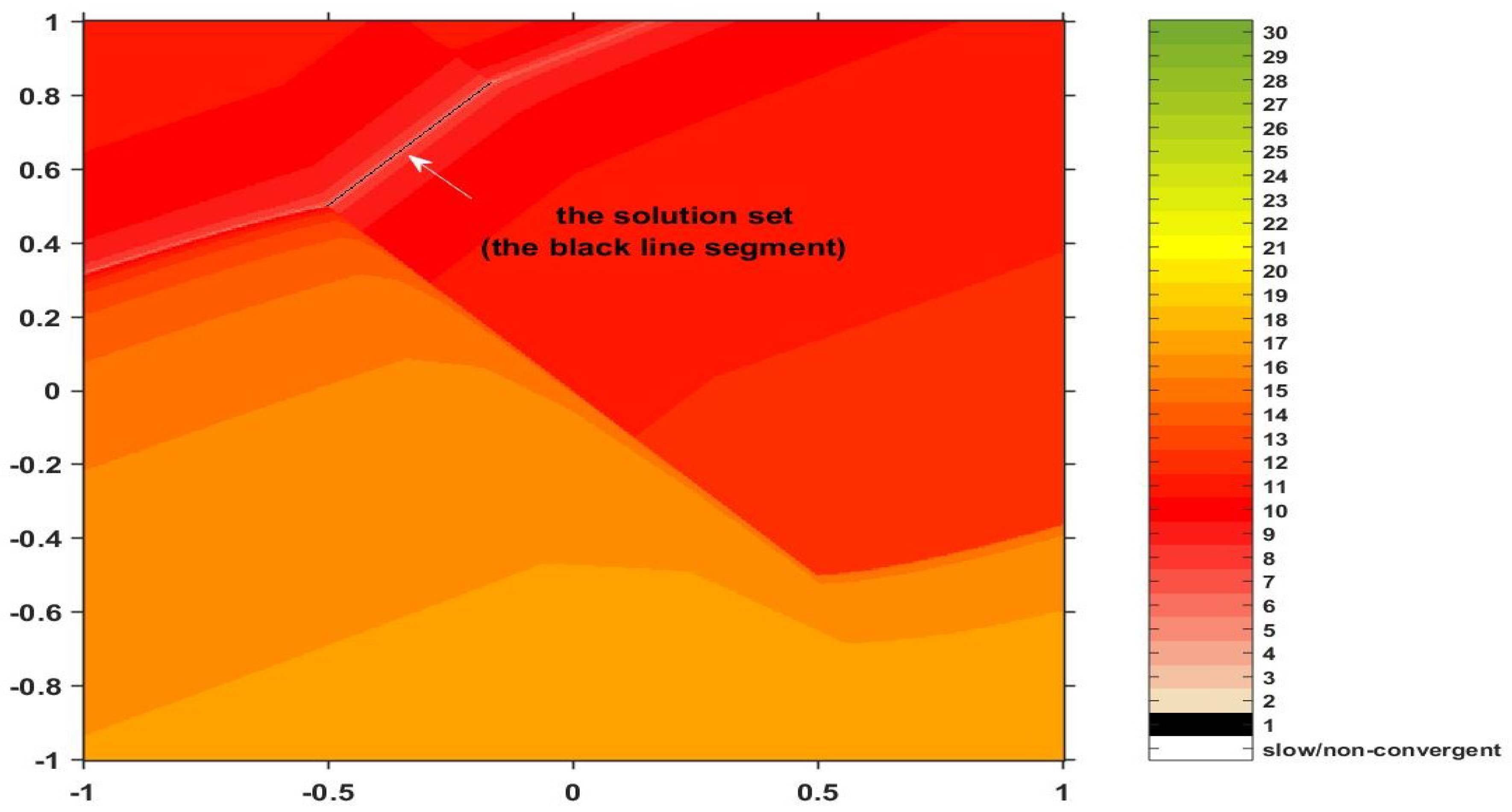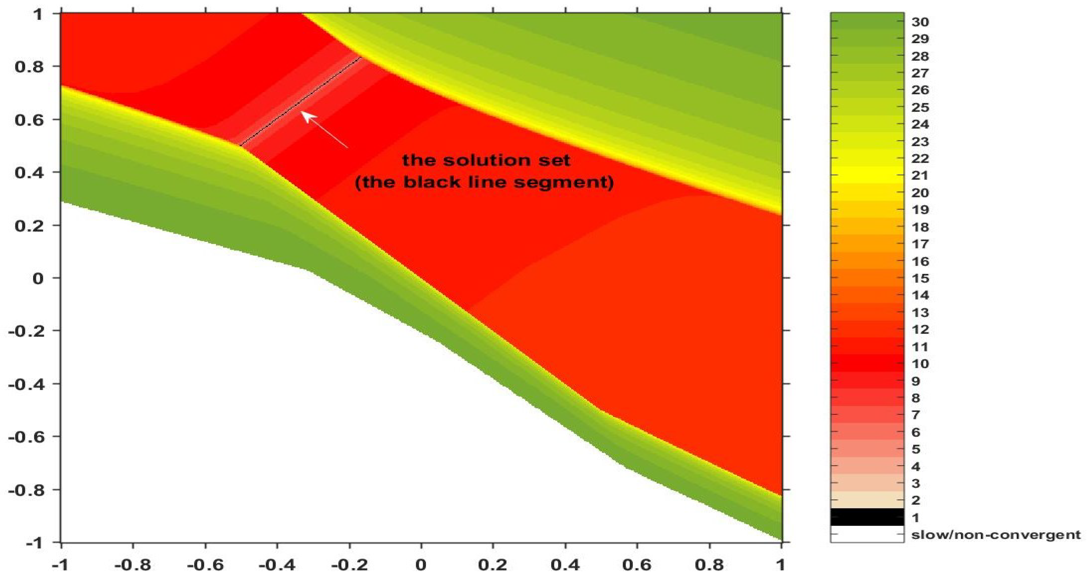Generally, this means that instead of analyzing the resulting approximate solutions and the required number of iterations starting from a single particular initial estimate $x_0$, we will choose an entire region of ${\mathbb{R}}^2$ and take each point of the region as a starting point. Then, for each such initial approximation, we count the number of iterations required for its orbit to reach a system solution. Depending on this number, we assign to that particular starting element a color. The color–number correspondence is usually set through a colorbar that accompanies the picture. The result is a colored image in which the particular color of a pixel encodes the number of iterations needed to obtain a solution when the algorithm is set to start from that point. Obviously, the color corresponding to one iteration will define the solution set itself.

In our example, we choose the region enclosed in a square set to $[-1,1]\times [-1,1]$ and we set the inputs for the algorithm as follows: the admissible error controlling the exit criterion is $\epsilon ={10}^{-5}$; the iteration step coefficients are set to be constant ${\displaystyle {\alpha }_n={\beta }_n={\gamma }_n=\frac{1}{2}}$ for the Prox-TTP procedure and ${\displaystyle \gamma =\frac{1}{8{∥A∥}^2}}$ for the Prox-Standard procedure; and the resolvent parameter is chosen $\lambda =1$. In addition to the error-related exit command, we consider an extra stopping condition: if the given accuracy does not result after 30 iterative steps, the algorithm is set to break. This helps us to avoid infinite loops or very slow processes corresponding to those initial points which generate slow-convergent iteration sequences. For these points, we supplement the colorbar with white. We also assign the color black to points for which only one iteration is required (the approximate solutions). The resulting polynomiographs are included in Figure 1 and Figure 2.

Analyzing the two images, the most important conclusion refers to the system solutions. As expected, both algorithms provide the same image of the solution set (the segment marked by the dark line). Moreover, apparently, the TTP procedure is more efficient because it generally uses colors from the bottom of the palette, while the standard procedure also uses colors from the top as well as white (indicating slow convergence). However, we must not forget that these images resulted for a particular selection of inputs ($\lambda$, ${\alpha }_n$, ${\beta }_n$, ${\gamma }_n$, $\gamma$ and $\epsilon$). It is not excluded that, by choosing the entries differently, the standard procedure is to become more efficient.

5. Conclusions

The standard algorithm that Moudafi suggested for the split variational inclusion problem includes two control parameters, $\gamma$ and $\lambda$. This means that, by simply adjusting the values of the parameters, one could obtain more efficient procedures. It is natural to think that the performance could be even better controlled if more parameters are involved. The three-step iteration procedure we analyzed here included four control inputs: $\lambda$ and the iteration coefficients ${\alpha }_n,{\beta }_n$ and ${\gamma }_n$. We proved next, using polynomiography, that a particular selection of these parameters improves the general convergence trend of the approximating sequences. More importantly, two new types of systems have been addressed as examples of SMVI problems; they combine an optimization problem and a linear subsystem, respectively, with a feasibility condition. For a particular selected experiment, we proved that the standard Moudafi procedure, as well as the newly introduced algorithm provide similar images of the solution set.