Abstract
This paper presents a methodology involving the transformation and conversion of qualitative data gathered from open, semi-structured interviews into quantitative data—a process known as quantitizing. In the process of analysing the factors behind the different levels of success in the implementation of entrepreneurship education programs in two case studies, we came up with a challenge that became the research question for this paper: “How can we best extract, organize and communicate insights from a vast amount of qualitative information?” To answer it, we developed a methodology involving codifying, labelling, attributing a score and creating indicators/indexes and a matrix of influence. This allowed us to extract more insights than would be possible with a mere qualitative approach (e.g., we were able to rank 53 categories in two dimensions, which would have been impossible based only on the qualitative data, given the high number of pairwise comparisons: 1378). While any work in the social sciences will always keep some degree of subjectivity, by providing an example of quantitizing qualitative information from interviews, we hope to contribute to the expansion of the toolbox in mixed methods research, social sciences and mathematics and encourage further applications of this type of approach.
Keywords:
quantitizing; qualitative data; aggregation of information; matrix of influence; mixed methods research MSC:
03-02
1. Introduction
The following text will lay out how we designed the integration of qualitative and quantitative data in the context of a research in the field of social sciences and propose how such a model may become paradigmatic in future studies that deal with vast data and case studies underpinned by interviews.
The object of our study was understanding the reasons behind the different levels of success in the implementation of entrepreneurship education programs (henceforth EEP) in Portugal, for which we considered two case studies, to provide an appropriate basis for comparison. To answer the research question behind this paper—“How can we best extract, organize and communicate insights from such a vast amount of qualitative information?”—and given the complexity, vastness and subjectivity of the object of study, we chose to transform the qualitative data through an appropriate sequence of steps, including (i) defining the concepts being studied, (ii) constructing indexes and indicators and (iii) creating a summary matrix of influence that would provide, in a visual manner, a clear characterization of the two case studies at hand.
We will also highlight why it is important to use a mixed methods design approach in social sciences to give breadth and scope to studies in this field. In brief, what we conducted can be decomposed in two stages. First, we quantitized data gathered from 39 interviews and followed a three-step approach in order to achieve more qualitative results, by organizing and quantitizing the information present in the 3749 quotes we extracted from those interviews. Second, to tackle the issue of implementation of entrepreneurship education programs, we used four important quantification tools: the Index of Average Presence Index (IAP), the Indicator of Average Magnitude (IAM), the Index of Criticality (IC) and the Matrix of Influence (MI). Indeed, these indicators converge to a summary Matrix of Influence that provides a visually clear characterization of the two case studies at hand. As we will see, this methodology builds up and gains consistency with every step. Because of this, what began as research relying predominantly upon qualitative data, our study went through a process in which the data became quantitized and the indicators revealed with more detail and mathematic accuracy what qualitative inputs would show.
Why not use a quantitization process tout court? Quantitative research—latu sensu—is, in its nature, essentially oriented towards verification, explanation and confirmation, within its frameworks of understanding of reality. Moreover, quantitizing is a methodological intervention directed towards engineering data to fulfill what may seem to be opposing purposes, including the reduction and amplification of data, in addition to the clarification of and extraction of meaning from data [1]. That is why the measurement of concepts, the search for causality, generalization, replication and validation as guiding principles are predominant [2,3,4,5,6]. In the research carried out, much of the initial inputs were mainly qualitative and with a high degree of subjectivity. Thus, the quantitative analysis of the interviews could only be achieved through a quantitizing process [7]. According to Gale et al. [8], “Qualitative data are voluminous (an hour of interview can generate 15–30 pages of text) and being able to manage and summarize (reduce) data is a vital aspect of the analysis process” [8]. This was certainly our experience.
The use of mixed methods research has been used for decades and has sprawled to practically every field of knowledge or research that intends to explore a broader scope, reduce subjectivities or compensate for the limitations of either qualitative or quantitative approaches alone. Our case revolved around the intensive use of contents of interviews and documentation analysis that related to social phenomena, i.e., decision-making processes. Although these methods may provide us with an overview of the matter at hand, interviews and analyses may give us impressionistic and somehow biased results. This means that a purely qualitative inquiry may only take us so far in understanding the problems surrounding our research object. This situation is common in social sciences and humanities, given that these fields usually use methods that privilege qualitative approaches and methods to carry out those approaches.
Qualitative research seeks to deeply understand a research subject rather than predict outcomes [9,10]. Thus, qualitative research values people’s lived experiences and is inherently subjective and sensitive to the biases of both researchers and participants [10,11]. Our choice for a mixed methods approach was made for its ability to tackle two main issues that we came across in the abovementioned research: the need for a readable systematization and effective management of data; to mitigate the subjectivity inherent to qualitative data [6,12,13]. Therefore, despite their ontological and epistemological differences, our combining of qualitative and quantitative methods in a single study seemed viable by employing an overarching paradigmatic model/framework [14,15].
Ultimately, the research performed adopted a mixed methods approach, based on an exploratory sequential design [16], as we will see next. In other words, we used predominantly qualitative data, which, in turn, went through a quantitizing process. As supported by Sandelowski et al. [1], this quantitizing serves as a way to think about and interact with data, so, in our case, this process enabled us to carry out a more thorough interpretation of the qualitative data gathered through semi-structured interviews. From our knowledge, our approach is novel to the literature. In all the papers we had the chance to read that deal with the quantitative treatment of qualitative data from interviews [1,7,17,18,19,20,21,22,23,24,25,26,27,28,29], the analysis offered is based on the transcription, codification and interpretation of the quotes, without taking the step of quantifying any of the qualitative information obtained. In other words, researchers usually use a qualitative analysis of content (which includes counting frequencies after the coding stage). We intend to take this further and will use the aforementioned example to show the blueprint of how this process can be performed in research that uses interviews.
2. Background and Theoretical Model Adopted
2.1. The Study
The main goal of the background research that used the methodology we are exposing here was to determine what were the conjunctures (and what factors inside each conjuncture) that lead decision makers to choose a certain path. The qualitative data that we will refer to often throughout this paper can be divided into two main strands: documentation and semi-structured interviews.
The reason of being stems from an inquiry to understand the conditions in which decision makers were likely (or favourable) to the implementation of entrepreneurship education programmes (mainly at NUTS III level and during compulsory school). The Nomenclature of Territorial Units for Statistics (NUTS) III corresponds, in Portugal, to a region or territory locally known as Intermunicipal Community (known as CIM). We will analyse two NUTS III: the CIM Viseu Dão Lafões (CIMVDL) and CIM Baixo Alentejo (CIMBAL). In addition, there are also allusions to the Portuguese case in general. The former was chosen because they allow considerable contrast, namely due to the results observed in terms of implementation and success of EEP. The national case remained a key element in our analysis as it enriched our comprehension of the relevant factors to be considered when studying the EEP implementation in the two regional cases chosen for a comparative study. While this topic is very precise—that is why we will minimise information that is less relevant since we want to highlight the methodological aspects involved in our research—the understanding of decision making has broader implications and ramifications and, thus, contributions from this study may help future research in this realm.
2.2. Sources of Information
The main sources of information regarding the implementation of the EEP were documentation and interviews. These were particularly favoured because in qualitative research, the interview, especially in its semi-structured form, has been regarded as an important technique since it allows to experiment and to tackle the context surrounding the subject, enabling the discovery of elements and categories that may reinforce and restructure the research goals [6,30,31,32]. Given that we were comparing two seemingly very different cases, we identified the need to obtain information from several different people involved in the decision process, as well as go through a triangulation process.
The qualitative nature of the information collected, particularly the 3749 quotes obtained from the 39 interview transcripts, created a need for a systematic treatment of the opinions expressed in them, as well as a theoretical support to frame and organize the amount of content collected. We extracted quotes after transcribing an interview. They were extracted after analysing the content, context and underlying intentions of the respective interviewee, and the identification of interesting segments of text that we call coding units. It is each of these text segments/coding units that we coded in step one (as explained next), in the categories of each of the theoretical frameworks that constitute the conceptual model adopted [8,30].
The interviewees assume a central role as sources of information. They are the ones who enform the practices of organizations and, through their personal constructs and theories, model their own practices; they are agents of social dynamics [33]. In order to have access to relevant information, we interviewed key informants who provided us with important data on the object of study in an interactive and holistic perspective [34]. The following key informants or potential informants [30,35] and privileged witnesses [36] were interviewed in our study due to their role in decision making concerning the implementation of EEP in schools: local mayors; presidents of Intermunicipal Communities; politically appointed decision; middle managers of the Intermunicipal Communities; school principals.
An interview script [6] was devised and used in every interview. This helps the comparison and structuring of the data. Therefore, the conduction of the semi-structured qualitative interviews resorted to the design of three grids, based on the items contained in each of the theoretical models adopted and explained below in point 2.3. The semi-structured interviews consisted of open questions to make it easier for the revelation of empirical data [37].
The preparation of the interviews involved the fulfilment of methodological requirements. Namely: guaranteeing the anonymity of the source of information; recording the interview and transcription to digital support; returning the text to the interviewee to validate it. The 39 interviews were recorded, and the duration varied according to the pace of each interviewee. The average time was 60 min. The process of managing and organizing the data, bearing in mind the high number of interviews and extensive documentation collected, was ensured through the preparation of a “file” in digital format (Microsoft Word) that served as an exhaustive database for each case.
2.3. Methodological Background
Understanding the decision-making process that underlies the implementation of Entrepreneurship Education Programs in compulsory education is a complex issue. It encompasses several aspects, which range from the scheduling and formulation of public policy to decision making and implementation. Howlett et al. [38] recommend dividing the study of public policy problems into three distinct but complementary phases:
(…) the ease provided by the understanding of the public policy process unfolded in parts, in which each of them can be investigated in isolation or in terms of its relationship with the other stages of the cycle, allowing the integration of empirical materials derived from the individual cases, the comparative studies of several cases and the study of one or more stages of one or several cases in political theories and analyses.
Based on this principle, we proceeded to deconstruct the public policy process in the following stages: (i) “Agenda”—a “pre-decision” phase; (ii) “Decision”—thought around the problem of the “decision” making phase; (iii) “Implementation”—referring to the “post-decision” phase. In the ambit of the literature review on theories/models that contribute to the understanding of public policies, the question arose of which theories/models to adopt as a reference for each stage. The whole process is explained in [39]. What follows is a contextualizing summary.
The choice considered two main criteria: on the one hand, the theoretical suitability of the models studied; on the other hand, the possibility of structuring and sectioning them, in order to allow a more detailed analysis—and, sometimes, necessarily compartmentalised—of the same. This second criterion is important given the complexity of the phenomenon under analysis, which results from the number of actors involved, timespan and vast legislation, institutions and communication links—all elements tied to the nature of multilevel governance associated with the management of the public policy cycle in the context of the implementation of EEP.
Based on these criteria, and on the premise that when used effectively (specifically by experienced and subject matter experts), this type of method is a systematic and flexible approach to analysing data and is appropriate for use in research [8]. The theoretical frameworks adopted in each of the stages are as follows: (i) Agenda stage (A)—“Multiple Streams Framework” [40] (Kingdon, 1984); (ii) Decision stage (D)—“Muddling Through Framework” [41,42] (Lindblom, 1959, 1979); (iii) Implementation stage (I)—“Implementation Analysis Framework” [43] (Sabatier and Mazmanian, 1980). The conceptual framework adopted—which is shown in the Figure 1—is in an integrated and coherent scheme (which contributed to the understanding and explanation of which forces and factors operate at each stage of the public policy cycle).
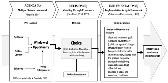
Figure 1.
Adopted Framework. Source: [44].
The approach described in the previous figure provides a framework that aims to identify (i) the processes that have to take place for an issue to enter the political agenda; (ii) how the various institutions proceed to decision making; (iii) how they carried out the implementation of a chosen public policy.
2.4. Constitutive Elements of the Conceptual Framework
In order to fulfil the objectives of the research carried out, two sub-levels of analysis were created within each of the theoretical frameworks adopted, which we called “Dimensions” and “Categories”. These constitute the organizing axes of the indicators and indexes that, in turn, make it possible to highlight the most important/critical factors for the successful implementation of public policies in the field of entrepreneurship education.
In line with Bardin [45] (2018), the dimensions were constructed based on the constitutive elements of each of the theoretical frameworks adopted, i.e., on the components defined according to the key idea attributed to them by their respective authors—five fundamental components in Kingdon’s theoretical model [40], six conditions associated with Sabatier and Mazmanian’s model (1980) [43] and five dimensions that capture the essence of the theoretical model developed by Lindblom (1959, 1979) [41,42]. In turn, each of these 16 dimensions were broken down into 53 categories or, more specifically, into 22 categories in the Agenda stage, 16 in the Decision stage and 15 in the Implementation stage, as can be seen in Tables S1–S3 in Appendix 1 of Supplementary Materials.
Indeed, this model allows the possibility of structuring and sectioning each of the three stages of decision making in order to allow a more detailed—and, often times, compartmentalised—analysis. The compartmentalisation aspect is key to our goals, as the next section will clarify. Each model is broken into dimensions and, within them, categories. Altogether, the three models comprise 16 dimensions and 53 categories—the latter being the main element upon which the whole process of quantitizing qualitative information was performed.
Figure 2 depicts the “skeleton” of the theoretical framework adopted, where its components become clearer: three stages, sixteen dimensions, fifty-three categories. As we will see, the process of quantifying the qualitative information will begin with “codifying” the quotes from the interviews, which is nothing more than placing each of them in one of the fifty-three “drawers” of the picture below. We exclude from here detailed descriptions of each element of the theoretical framework adopted to keep the presentation as succinct as possible and because the content relates to political science and public policy. A more interested reader can consult [39], where the process of choosing, integrating and making sense of the three models chosen, as well as comments on each dimension and category included in it are thoroughly explained.
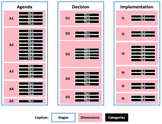
Figure 2.
Skeleton of the Theoretical Framework adopted. Source: the authors.
To clarify the framework, we give two examples. The Agenda stage has five dimensions (A1 to A5) and the first dimension (A1) has four categories in it: A1.1, A1.2, A1.3 and A1.4. The Implementation stage has six dimensions with the fifth (I5) including two categories (I5.1 and I5.2).
3. Methodology
In order to analyse the content of the interviews carried out, we defined a methodology to transform the qualitative data in quantitative indicators and indexes, adopting a sequence of steps, beginning with the codification of the quotes; secondly, with the choice of a qualitative label, followed by the attribution of a score; thirdly, by constructing indexes and indicators from these scores, as shown in Figure 3.
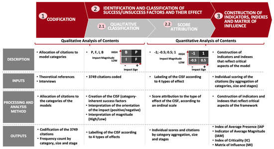
Figure 3.
Steps adopted in the Quantitization of the Qualitative Data from Interviews. Source: the authors.
3.1. The First Step (1)—Codification
By codification, we mean the allocation of each of the selected quotes to one of 53 categories [31] of the integrated framework presented earlier in Figure 1. This process involves a qualitative content analysis of each quote and thoughtful consideration of which category in the theoretical model selected shows a better fit, according to a set of criteria defined in the literature [6,29,45,46,47,48].
To illustrate this first step, we provide an example:
“We are helping our students to acquire knowledge, stimulate their attitudes and develop their entrepreneurial skills. These will be very useful when it comes to adapting to the job market and the challenges it presents.”
This quote was allocated to category A2.5—Compatibility with values. This was performed for the remaining 3748 quotes. Following the best practices in codification, we used the NVivo software to record the content analysis and to keep the process clear, consistent and easily traceable. We believe that different researchers would reach similar results if they proceeded to categorise the same content units, based on the aforementioned rules and the chosen theoretical framework. In other words, we maximized the mitigation of issues of subjectivity. The Figure 4 is taken from the NVivo software, where we can observe the structure of the theoretical framework adopted.
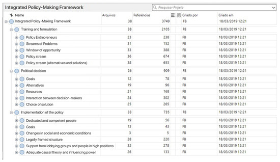
Figure 4.
Snapshot of the NVivo Software. Source: the authors.
The breakdown of the 3749 coding units (by stage and case) is shown in Table 1.

Table 1.
Quotes per Stage and Case Study.
The distribution of the 3749 quotes by case is as follows: 1070 for the National case (29%), 1527 for the CIMBAL (41%) and 1152 for the CIMVDL (30%). This distribution is largely influenced by the number of interviews carried out for each case: 8 in the National case, 19 in the CIMBAL and 12 in CIMVDL.
The frequency count—the number of quotes—is extremely valuable because it is quite objective. It constitutes, to paraphrase Bardin [45], a first step in the content analysis, allowing the researcher to obtain a first impression of the relative importance of the elements of the theoretical framework adopted. The Frequency Count Indicator (FCI) will also be relevant for the quantitization of the qualitative data, in that the number of quotes in each category will be the obvious weight to consider when performing averages for the other elements (dimensions and stages).
3.2. The Second Step (2)—Identification and Classification of Success/Failure Factors and Their Effect
This second step is divided in two: the qualitative classification and the attribution of a score (steps 2.1 and 2.2 in Figure 3). Since our aim is to study the relevance of different elements for the success of the EEP implementation, upon codifying each quote, we had to give a label to each quote. Thus, we had to define previously the concept of success (in the context of this study) so that it may be classified and subsequently measured [12,49,50,51]. Our goal is to understand what contributes for the success in each of the three stages of the public policy cycle. Success in each stage is necessary for the overall success, i.e., the effective implementation of EEP. We synthesize the information on success in Figure 5.
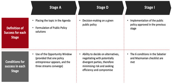
Figure 5.
Definition of Success and Conditions for it to Happen in Each Stage. Source: the authors.
Considering the theoretical rationale proposed for the definition of success at each stage and that our aim was to understand whether the key success factors underlying the category to which the quote was allocated to were present or absent and the magnitude/impact of its presence/absence, the need for data treatability made evident the necessity to create a new variable that could be measured and allow for a better understanding of the theoretical concept desired [12]. This new variable came to be the Category-Inherent Success Factor (CISF) and constitutes, using Bardin’s terms [45], a (new) “unit of context”, enabling us to face the existing ambiguity in the referencing of the meaning of the coded elements so that the analysis could be consistent and productive.
The CISF, therefore, clarifies the key success factors underlying each category. The quote we used as an example above was allocated to category A2.5–Compatibility with values. How could we put a label on a quote based on such a neutral description? We had to write an appropriate CISF for this category, which came to be the following:
“A reasonable/high alignment between the proposed solutions to the problem and the values of the relevant community (family, school, company, neighbourhood, city, CIM, region, etc) elevates the consensus around the importance of the solutions.”
To allow better visualisation of our point, in Table 2, we will illustrate, with 5 examples, how the creation of the CISF makes the success factors clearer:
Table 2.
Some Examples of Categories and their CISFs.
Considering the above, it becomes noticeable that the inclusion of this new variable allows for standardisation in the approach of each of the 3 models, insofar as the formulation of each of the CISF makes clear what is beneficial for success in each of the stages for the respective category. Thus, this variable, the CISF, was uniformly worded so as to be an affirmative statement that describes the elements necessary for success in a stage, in terms of the category to which it relates. As we will see, the creation of the CISF also allows us to deal with the issue of having categories with a positive, negative or dubious impact when these categories are present.
In summary, if this operation of standardising the categories was not carried out, the researcher would face the difficulty of interpreting the content of the coded quote. This would be particularly troublesome in cases where some categories have such characteristics that they can assume three types of connection with success in the stage—positive, negative or dubious. We use the term connection to mean how success in a stage varies when the “quantity” of the category “increases”. For example, for category I5.1, what happens when the “Formalization of Support” is greater? Does success tend to increase (positive impact), tend to decrease (negative impact) or does it depend (dubious impact)? For D4.3: what happens when cultural idiosyncrasy “increases”? What is the meaning of the impact on the success of the stage of having a “greater amount” of cultural idiosyncrasy? This new variable always has a positive impact when the CISF is present and a negative impact whenever the CISF is absent. Another example: in the “Financial Viability” category, in the “Policy Flow” dimension A2 of the Kingdon model, a category with a positive impact, the corresponding CISF assumes the following description: “Financial viability in the solutions proposed to solve the problem”. The “Restrictions to the System” category, in the same A2, with a negative impact, has as CISF “Decision-makers are able to anticipate future restrictions to their proposals”.
The CISF also allows to deal with dubious categories where the impact of a “stronger presence” of the category, as it is described, is not necessarily positive or negative. For example, the category “Governmental Changes”, in the A3 dimension, “Policy Flow”, of the Kingdon model has as CISF “There are people in strategic positions in the decision-making structure favorable to the entry of the topic on the Agenda”.
3.3. Classification of the Type of Effect of the CISFs
The conceptual framework adopted that we have been following to identify and classify the critical success factors, by itself, does not translate the dynamics that these factors reveal. Therefore, we resorted to another model in the area of management, the Force Field Analysis. It is this model that will allow us to revisit the CISFs and interpret them according to the type of effect they have on the various stages of the policy cycle. This effect is classified into factors that drive/enable the process, or, in contrast, restrain or block it. It is this type of effect that we present in the following figure.
Bearing in mind the rationale present in Figure 6, it is now important to exemplify how we used in a practical application when we had to interpret any given “quote” according to the effect it had on success in the stage to which it corresponded, i.e., Agenda, Decision or Implementation.
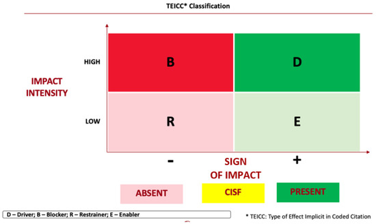
Figure 6.
Classification of the Type of Effect of the CISFs. Source: the authors.
In this context, we had to interpret as faithfully as possible the quote that the interviewees said and its context. We took into account the effect on the success of the stage, as well as the meaning and intensity of the impact. In other words: whether it is positive or negative and if the stance is of high or low magnitude. Thus, when a certain interviewee talks over a period of time, for example, about the position of their institution regarding the placement of EEP on the agenda, we immediately placed/coded the quote in category A3.3—Position of the institutions involved—and then, qualitatively classified the type of effect inherent to the coded quote (CISF), according to the reference in the two dimensions adopted to carry out this classification.
Being aware of the importance of this procedure during the qualitative analysis of the content of the interviews carried out, we considered useful the reinforcement of the practical exemplification of its application through the presentation in Table 3 of the coding of 4 quotes and their subsequent classification according to the type of effect for success of the CISF Driver, Blocker, Restrainer and Enabler
Table 3.
Four Examples of the Process of Codification and Classification.
Based on what is explained above, it is possible to observe and interpret in Tables S1–S3 in Appendix 2 of Supplementary Materials how the qualitative classification of all CISFs was made, i.e., of the type of effect inherent to the 3749 quotes spread throughout the three stages. We can also conclude that the qualitative content analyses of the interviews come here to an end. The ensuing phase corresponds to quantitative analysis, as explained in Figure 3.
3.4. Quantitative Analysis
After we have defined and classified the type of effect inherent to FSIC, in terms of the meaning and intensity of its impact, it becomes necessary to choose/develop appropriate instruments that help us measure [12] some aspects that contribute to the understanding of the matter at hand. The question then arises of which indicator to build and which operations should be carried out, in order to guarantee the desired quality in the research process, since the way in which concepts are defined and measured impacts the validity of research results and, consequently, the theoretical validity of the study [12].
3.4.1. Theoretical Meaning of Indicators
The conceptual definition provides the theoretical meaning of a construct and guides the development or choice of the appropriate indicator to measure the concept [49]. In our case, we established that our object of analysis is to understand what contributes to success in each of the 3 stages of the public policy cycle. A summary of this can be found in Figure 3.
3.4.2. Measuring the Indicators
According to Fortin [12], the measurement can be defined quantitatively—through the attribution of numerical values to objects or events according to certain measurement or correspondence rules—or qualitatively, through a classification process which consists of assigning numbers to categories to represent variations in the studied concept.
The attribution of numbers to the classification of the type of effect implicit in codified quotes, presented in the previous tables, was carried out in line with Krippendorf [52], who also considers it convenient to assign numbers to categories in order to support the interpretation of variations in the phenomena.
Before describing the measuring scale adopted for the attribution of these numbers, it is important to reinforce that, according to Fortin [12] and Saldaña [53] (2013), measuring consists of attributing numbers to objects or events according to certain rules. According to these authors, the value that an attribute has can be represented with four measurement scales in ascending order, as follows:
(i) The nominal scale, which serves to assign numbers to objects to represent mutually exclusive and exhaustive categories. (ii) The ordinal scale, in which numbers are assigned to objects representing an order of magnitude. Because these numbers represent a rank and not absolute numerical quantities, this scale does not allow these numbers to be added or subtracted. (iii) The range scale, which ensures continuous values and, in which, the assigned numbers, being spaced at equal intervals, can be added or subtracted. Finally, (iv) the ratio scale, with intervals and an absolute zero to represent the absence of the phenomenon.
3.4.3. Score Attribution
Based on the previous conclusions and guiding our step 2.1 (qualitative classifications of Figure 5), and having built the category-inherent success factor variable, it became clear that it would be appropriate to opt for the use of an ordinal scale with 4 values that reflect the types of the aforementioned classification. On the other hand, as the impact of some variables is positive (when they are more present or present to a greater degree/intensity) and in others it is negative, we also chose a scale with positive and negative values. The values of this scale are symmetrical, insofar as the impacts are of the same nature, whether positive or negative. Given that our approach was essentially inductive, pragmatic and in line with the objectives of the analysis, and since the researcher can see some differentiability in the statements collected, it would be limiting to consider only a scale with two values (one positive and one negative). Thus, we chose a scale with two positive values and two negative values, as shown in Table 4.
Table 4.
Type of Classification Ordinal Scale.
We, therefore, considered it appropriate to have the minimum number of values on a symmetrical scale that allowed having more than one positive/negative value.
Since we intend to study the extent to which the CISFs were present or absent, it becomes possible with this scale to provide a clear reading of what was classified as reflecting the presence or absence of the respective CISF. As far as magnitude is concerned, given that it was decided that the qualitative classification of the CISF would consider two types of magnitude, it became necessary to answer the question of how to adequately reflect its impact on the scale.
For the sake of standardisation, we opted for a scale between −1 and 1. These values correspond to the extreme classifications that, in the model presented above, refer to the types of effects implicit in quotes coded with high magnitude, respectively, Blocker and Driver. Although there is no neutral element in the classification of CISFs, we adopted, for classifications with low magnitude, values that are equidistant from this tacit reference. Since a neutral stance is absent from the model, it is, in a certain way, omnipresent. It is not only the intermediate point between the extremes of the scale, but also the point at which there is a change, not of degree, but of a qualitative change in the CISF, from absent to present.
Therefore, it is natural for us to attribute to low magnitude CISFs the intermediate value in the range where the CISF has the same quality, i.e., the CISF has a positive impact on the [0,1] range and a negative impact on the [–1,0] range. This brings about the values of −0.5 and 0.5 attributed to low-magnitude CISF, thus reflecting the absence or presence of the CISF—which we have designated, respectively, as Restrainer and Enabler for the success of one of the three stages. The blocking factor does not block, as in a “veto”; it works instead as a “stronger brake”. It is thus entirely symmetrical to the driving factor, and not a binary factor (as it would be if it were like a “veto”).
Still concerning the absence of a “neutral” element on the aforementioned scale, it is important to note that this fact occurred to the extent that all the evidences collected (the coded quotes) pointed to a positive or negative impact. In the interviews, the interviewees mentioned “relevant” events, i.e., events that contributed, from their point of view, positively or negatively to successes or failures, and not “irrelevant”, neutral events.
Another methodological question that we were faced with has to do with the distance between the elements of the scale. According to Fortin [12], although the values assigned to designate the respective categories of the scale can be arbitrary—as long as they respect a certain logic that allows placing the variables among themselves—the spacing between two scale values is not necessarily constant. However, according to Fortin [12], in cases where the choice of scale does not greatly interfere in the results, a situation that occurs when the frequency distribution does not possess a great bias, constant distances between 4 elements (for example, with values of 1, 1/3, −1/3 and −1) are a viable option. Within the scope of this work, we chose to maintain the scale presented above.
3.4.4. Construction of Indicators, Indexes and Matrix of Influence
For the purpose of this paper, the term index is understood as a numerical value that represents a composite variable, quantitatively and thematically consistent, from the calculation of sums or averages of the scores of the categories that served as input to the respective calculation. We will present a composite index resulting from 2 indicators: (i) one based on the relative frequency of the categories, i.e., the relative frequency of one category against the others; (ii) Average Magnitude (henceforth AM), that is, the Average Presence (henceforth AP) module (which is between 0.05 and 1) standardised to 0 to 1, allowing to obtain the % of quotes of high magnitude.
Even though we are aware that even in exact sciences the development of quantitative indicators is a considerable challenge [54]—and that its implementation in the scope of the human and social sciences becomes even more difficult—we considered it possible to carry out a systematic construction of quantitative indicators for our investigation process. Moreover, we consider this to be a best practice since the adoption of composite indicators has been gaining more and more popularity in recent times, with various authors contributing new methodologies on this topic over the past years [55].
For the AP and AM indicators, which will be presented and described below, the essential properties that any indicator must present were considered [54] within the scope of the process to which it refers:
- (i)
- Relevance—portrayal of an important, essential aspect of the process;
- (ii)
- intensity grading—sufficient variation in the process space;
- (iii)
- univocity—portraying with complete clarity a unique and well-defined aspect of the process;
- (iv)
- stability—be based on a well-defined and time-stable procedure;
- (v)
- traceability—the data on which the indicator is based and the calculations performed must be recorded and preserved.
We believe that the two indicators that were elaborated and we will present next can be considered, according to Jannuzzi [56], methodological assets that add value to the content analysis performed since it contributed to quantifying and operationalizing abstract social concepts of theoretical interest (for the academic research) or programmatic (for policy making).
These indicators are examples of analysis techniques built in a systematic way, using clear and well-defined analytical operations. Their goal is to contribute to the explanation and systematization of the content of the messages, in line with what Bardin [44] suggests.
3.4.5. Index of Average Presence
Building up on previously mentioned information, we have conceived the Indicator of Average Presence (IAP).
In short, the construction of the IAP—for categories, dimensions and stages—gives us the chance to calculate weighted averages and the possibility to conduct ordinal analysis (of ranking, not of ratio) about those averages. Thus, through the IAP, it is possible to measure three main elements of our case studies: (i) what are the categories with more/fewer CISF? (ii) What are the dimensions with more/fewer CISF? (iii) What is the average presence in each stage of the public policy cycle?
This is a quantitative measure that produces a global score that reflects how present were the success factors in each level of the analysis—i.e., categories, dimensions and stages of the public policy cycle. This will provide us with a metric indicator of the success verified in the different levels of analysis mentioned when we carry out a comparative analysis of case studies—namely, the processes of implementation of education for entrepreneurship programmes in the Dão-Lafões and lower Alentejo regions. In this indicator, the scores given to the variables (at their most disaggregated level, which in our cases are the categories) have both ordinal and interval properties. This makes possible the calculation of weighted averages based on those scores, in order to obtain scores in the upper levels, i.e., scores for dimensions and stages.
The Average Presence of a given category—that is inside a dimension, which in turn is included in one of the three stages—is the weighted average of the scores given to quotes that were allocated to that category. This process can be seen in Table S1 in Appendix 3 of Supplementary Materials. This indicator is particularly useful to immediately see if a certain category/dimension/stage had a positive or negative score—globally reflecting if it had their respective CISF more present or absent. For a more detailed understanding of this step—if, for instance, we want to compare the IAP obtained for the Agenda stage in each case study—we may see the results in Table S2 in Appendix 3 of Supplementary Materials.
Considering that the Average Presence is the indicator of the degree of presence of success factors relevant for each stage, we can state that, in average, a higher AP is associated with a high probability of success in that stage. From the IAP we can make observations of ordinal nature concerning the probability of success in the corresponding stage. For instance, if in a certain case the AP in stage A is −0.22 and in another case is 0.15, we can say that the case with the higher AP should be associated with a higher probability of success. However, this is as far as this tool can take us. The IAP, built on the interval −1,1, does not have a reference point that may be associated with a concrete probability value (e.g., we cannot assert that an AP ≤ to 0.08 is associated with a probability of 0, or that an AP = 0 is associated with a probability of 0.5).
In conceptual terms, we can correspond the probability of success to each result. Considering how the API is constructed, we can associate a higher AP value with a higher probability of success. We can mathematically—and in abstract—translate that idea in the following expressions, in which f(AP) would be a function that would grant the probability of success depending on the AP value: (i) Prob (success) = f (AP); (ii) if a < b, then f(a) < f(b); (iii) f’ (AP) > 0. This idea—that a higher AP value could be associated with a higher probability of success—is illustrated in Figure 7
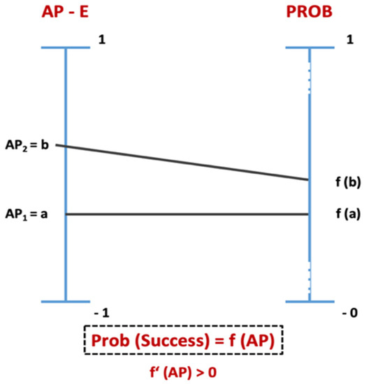
Figure 7.
Average Presence and Probability of Success. Source: the authors.
Finally, it should be highlighted that, despite the rigor present throughout the processing of the content of interviews (especially when it came to the melioration of the IAP), this quantitative tool (Average Presence) should be faced as part of the quantitization process of the qualitative data of the contents of interviews.
3.4.6. Indicator of Average Magnitude
Whereas the IAP synthesizes, for each element of the analysis, their performance in the horizontal axis of the CISF classification matrix, the AM synthesizes the performance obtained in the vertical axis of the matrix—which concerns the magnitude of impact (high or low) detected in the coded quote, therefore, revealing the average magnitude for that unit of analysis. This indicator gives us a measure to assess the impact of each element for the success of the stage in which it is inserted. The AM of each unit of analysis allows us to complement the information conveyed by the IAP, by revealing the impact that that unit of analysis had in the success or unsuccess of the stage in which it is inserted (being the success or unsuccess dependent on the orientation of the AP).
Like the AP, AM is also calculated, in the first place, at the category level. On Table S3 in Appendix 3 of Supplementary Materials, we have an illustration of the calculation made at the category level, for the A1 dimension categories—Problems in the National case. For instance, category A1.1 “Indicators” has AM = 0.40 which is a result of 2 quotes with high magnitude (score of 1) and 3 quotations with low magnitude (score of 0.5). A1.3 “Feedback of political action” has an AM = 0.31, which is the result of 5 quotations with high magnitude and 11 quotes with low magnitude. This method applies successively to other categories.
In a way similar to the one used to calculate the AP, the AM is calculated for each dimension through the weighted average of the AM value for the categories of that dimension. In this case (A1), that weighted average is 0.41. Finally, we have also calculated the AM of each stage by calculating the weighted average of the AM value for the dimensions that constitute that stage, weighted by the number of quotes pertaining to each dimension
In the National case, illustrated in Table S4 in Appendix 3 of Supplementary Materials, we can see that the AM of the Agenda stage is 0.55—a result where we can find the already-calculated value for the AM of dimension A1 (0.41).
With the aim of providing an easy reading of the results, we chose to standardise the AM value, resorting to a scale between 0 and 1. This makes AMi = Fi, that is, in a scale from 0 to 1 or between 0 and 100%, the AM value becomes equal to the percentage of quotes in that unit of analysis with high magnitude. This is easily perceptible if we consider that we are weighting the proportion of quotes with high magnitude (with score = 1, in the new scale) with the proportion of quotes with low magnitude (score = 0).
Thus, a category with a magnitude close to 1 is a category in which the underlying quotes has necessarily a large proportion of “1” and/or “−1” scores. In other words, either that the CISF existed and was very critical for success, or that the CISF did not exist and that determined failure. A category with a low AM, close to 0, will be a category in which the underlying quotes had a large proportion of “0.5” and/or “−0.5” scores. This means that the CISF had, on average, a lesser impact. To visualise the AM of each category, we present in Appendix 4 of Supplementary Materials a table with a ranking, in descending order, that reveals in a quick and practical way the categories with higher and lower average magnitude (already standardised in a [0,1] scale). This indicator is particularly useful given that it will be, in tandem with the Frequency Count Indicator, one of the inputs used to create the Index of Criticality (IC), which we are going to address next. Since this paper necessitates brevity, we will not expose here the outputs of the IC. However, the IC will be key to identify the categories/dimensions/stages with higher/lower impact/importance for the overall success in the implementation of education for entrepreneurship programmes in Portuguese schools.
3.4.7. Index of Criticality
The methods used to build the index of criticality (IC) obeys the ten-step process proposed by the Handbook on Construction of Composite Indicators [57]. In short, the IC is a composite index that is the result of the geometric average of two indexes: the Index of Frequency (IF) and the IAM, built from the blend of the IAM and Frequency Count Indicator (FCI).
In the context of the research, the purpose of the IC is to sum in a single indicator the importance/criticality of the constitutive elements of the conceptual framework adopted. The output is a ranking; a visualisation of the hierarchical importance/criticality that allows an ordinal reading of its results.
The IC, through the ordinal reading of the results, makes possible a comparative analysis between two (or more) elements of the selected sample. The reader will be able to know, primarily, the position in the IC ranking of each element and, subsequently, know the difference between other values for each element of the comparative analysis—such as IF/FC and IAM/AM. Concretely, the IC values per se allow (due to the way it is constructed) an ordinal interpretation (to have an idea of the importance of the respective variables); however, the interpretation of the registered differences will have to be conducted based on the IF values and IAM, given that these were the values that led to the IC calculation.
With regard to the interval in the IC, it varies from 0 to a not limited value because its components (FI and IAM) do not possess a cap value. In fact, both the IF and the IAM are based on a median of 100, so they are limited below 0, but do not have a cap value. Given that the IC is simply the geometric average of IF and IAM, there is no further treatment, i.e., the value of IC = 100 does not have, per se, any reference or value in the sample.
3.4.8. The Matrix of Influence
Considering the research in social sciences that was carried out and the case studies that support it (the national case and two NUTSIII cases), it is interesting to look at two already-mentioned indicators: the IC and the IAP. On the one hand, the IC tells how critical an element of the framework is, regardless of how present or absent it is. On the other hand, the IAP tells us how present/absent that element is, regardless of how critical it is. The natural question that arises from this is how we can aggregate both indexes. That is when we started to look at influence through the lens of the binomial Criticality|Average Presence.
The choice of building a matrix to integrate information of two indicators follows Verdinelli and Scagnoli’s suggestion [58] about the use of matrices as the best option to cross two or more dimensions, variables or relevant concepts of the topic being studied. This will not only make the understanding of the phenomena easier, but will also enhance the visual component in the communication of results. Indeed, the Matrix of Influence is a viable framework to synthesize information that we have gathered throughout this process.
Thus, for any level of criticality, the higher the presence or absence, the higher the influence. By the same token, for any level of Average Presence, the higher the criticality, the higher the influence. That is why we strive to obtain monotonicity concerning any of the two variables—i.e., that the variation is always in the same direction. However, given the complexity in aggregating these variables, we opted to use a qualitative indicator of influence—instead of a quantitative one—based on the Matrix of Influence presented in Figure 8 (which provides us with different levels of influence for the combination of values between the IC and the IAP).
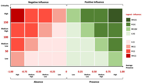
Figure 8.
Matrix of Influence. Source: the authors.
In the horizontal axis, we can find the Index of Average Presence (IAP). The scale is divided in 8 intervals: 4 intervals in which the values are positive (Presence) and 4 intervals in which the values are negative (Absence). In the vertical axis is the IC, which we have subdivided in 4 intervals. The colour coding, along with the respective legend, illustrates the four types of classification that we propose for influence: Very High (VH), High (H), Medium (M) and Low (L). Given that influence can be positive or negative, depending whether we have AP > 0 or AP < 0, influence can be of 8 kinds: VH (+), H (+), M (+), L (+), L (−), M (−), H (−) and VH (−). The value of this analysis translated by a qualitative variable is the way we found to integrate data contained in the CI and AP indicators in a comprehensible way that makes justice to the mixed methods approach that we have decided to adopt.
At this point, we ought to briefly recapitulate the main steps in three of the principal indicators used. The IAP measures the degree of presence/absence of the CISF, regardless of how critical they were. From that data we built, through the calculation of the weighted average, the degree of Average Presence for the elements that constitute the dimensions and stages of the exposed framework. The IC seeks to measure the criticality of the different elements of the adopted framework, regardless of their presence (absence). The Matrix of Influence can only be achieved when other indexes are attained. It combines the information provided by both the IAP and IC to characterize, qualitatively, the degree of influence that occurred in the case studies.
The following diagram, Figure 9, shows the overarching architecture of indicators and indexes use to build the Matrix of Influence of our methodological approach and how the different steps were achieved and created the possibility of progressing towards the making of a Matrix of Influence. It also identifies, for each of the components used in intermediate calculations, the object of measure and the qualitative or quantitative nature of that component.
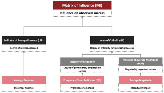
Figure 9.
Diagram of the Architecture of Indexes and Indicators to Build the Matrix of Influence. Source: the authors.
We will briefly recapitulate the three main indexes of the diagram.
- The Average Presence Indicator (IAP) measures the degree of presence/absence of category-inherent success factors that make up the model (the “CISF”), regardless of how critical they were. From these data, we built, through the calculation of a weighted average, the degree of average presence (AP) for the more aggregated levels that make up the dimensions and steps. It does so on −1 to 1 scale;
- the Index of Criticality (IC) seeks to measure the “criticality” of the different elements of the adopted model, regardless of whether they were more or less present or absent, and is built by combining the CFI and the AMI. It does so on a scale with a lower bound of 0 and no upper bound, in which the value 100 is assigned to the median;
- the Matrix of Influence combines the information provided by the IC and IAP to qualitatively characterize the degree of influence that occurred in the case studies. It does so on a scale of 4 levels—very high, high, medium low and low, and there can be a positive or negative influence, giving rise to 8 types of classification.
4. Results: Comparative Analysis of Both Cases—The Integrated Public Policy Cycle
In this section, we will analyse, in an integrated, measurable and as practical as possible way, the effect of actions and activities carried out by decision makers and agents throughout the public policy cycle. We used the indicators resulting from the methodology described above, which helped us to prioritize and highlight the most critical and influential elements in the design, decision and implementation of policies on entrepreneurship education programs. Our methods allowed a deeper and simultaneously aggregated understanding of the entire process. Our focus will be the analysis of the AP differential. This will enable us to see the contrast between success and failure in the two cases. We will complement our analysis with a look at the AM, FC and IC indicators for the levels of analysis “stage” and “category”. In addition, at a more detailed level—the categories—we will also look at the level of influence of each category and the difference in influence that occurred between the two cases.
4.1. Analysis per Stage
Let us start, then, by observing the data in Table 5, which show the results of the AP, AM, FC and IC indicators related to each of the cases.
Table 5.
Comparison of the CIMBAL and CIMVDL Cases According to the Four Indicators. Source: the authors.
First, the AP indicator presents a global differential for the set of the three stages of 0.93 with CIMVDL having an overall value of 0.77 and CIMBAL of −0.16 (numbers that reflect, respectively, the “success” and “failure” occurred). In fact, the CIMVDL case has the highest Average Presence value (of the success factors in each of the stages), indicating that this was the case that had the greatest success, contrasting with the failure observed in CIMBAL as a result of the global absence of factors of success.
Bearing in mind that the AP scale varies between −1 and 1 (therefore, having an amplitude of 2.00), a differential of 0.93 reflects a high gap in performance between the two cases. Looking now at the articulation of this global value, we see that the Decision stage is the one in which there is a greater AP differential—1.48—indicating that this stage was the most critical for the failure of the EEP policy in the Baixo Alentejo Region. In second, comes the Implementation stage with 0.86 and finally, the Agenda stage with a differential of 0.65. We can also observe that the CIMVDL’s degree of success is similar in the three stages. In the CIMBAL case, there is greater asymmetry with a very negative result in the Decision stage (AP = −0.63). We also note that CIMBAL has a slightly positive result in the Agenda stage (AP = 0.05) and slightly negative in the Implementation stage (AP = −0.03).
Using the data in Table 5 (above) to compare the performance of each of the cases, we observed that the differences in terms of the AM indicator in the three stages allow us to verify that in the CIMVDL case not only the success factors were present to a greater extent, but the impact of its presence was higher, given the values of AM between 70 and 85%, compared to the values in the CIMBAL case between 56 and 70%. The remarkable values of AM for CIMBAL indicate, given the negative (or almost) value of AP for CIMBAL, that the absence of success factors in these three stages had a significant impact on the overall failure observed in this region. This will become clearer when we address the category analysis level. Yet, it is important to point out that not only was the absence of the CISFs observed in the Decision stage, but this absence inhibited or blocked success in this stage.
Table 6 (below) includes six of the classifications of the type of effect of the CISFs inherent to the quotes of the Decision stage in each of the cases. Thus, the distribution of the 441 and 213 quotes pertaining, respectively, to the CIMBAL and CIMVDL cases, allocated to the Decision stage, is as follows:
Table 6.
Justificative Evidences of the Success/Failure in the Decision, Agenda and Implementation Stages. Source: the authors.
The asymmetry between the two cases is made clear in the lowest levels of the Decision stage, i.e., dimensions and categories. The amplitude of the differences between the CIMVDL and CIMBAL in the Agenda and Implementation stages (also in Table 6) are smaller compared to the Decision stage since the success factors in these stages were already present, even if in a slightly positive or even slightly negative way.
4.2. Analysis by Category
After analysing the results at the dimension level, it is now important to study the results at the category level. Following the example adopted for stage and dimensions, Table 7 presents the 53 categories of the proposed integrated model according to the AP differential ranking (CIMVDL–CIMBAL).
Table 7.
Success and Failure According to the AP Indicator in the 53 Categories of the Proposed Model. Source: the authors.
We thus observe that there are 23 categories in which, for the CIMBAL case, AP < 0 and another 30 in which AP ≥ 0. Within the categories that globally (and on average) reveal absence of success factors, we see that the differential is higher than 1.00 for 18 of them. More precisely and in descending order: D4.4; D4.3; D3.4; D3.1; I2.2; D3.2; D5.3; A3.2; D1.3; A4.2; D5.2; D2.2; A3.4; D5.1; I3.5; D4.1; I3.1; A2.6. We can also see that 11 of these 18 categories are part of the Decision stage. This is evidence that this stage was, according to our interviewees, the one that most influenced the failure verified in CIMBAL. Indeed, it was the one in which the absence of critical success factors was more evident—or, conversely, where a greater presence of factors linked to failure exists. In contrast, when analysing the CIMVDL data, we observe only two categories with PM < 0 (A2.9 and I6.2), while all other categories have AP ≥ 0.
As we had already observed in the analysis carried out at the level of dimensions, we can also see that in the CIMVDL not only were the success factors present to a greater degree, but the impact of their presence was higher. The AM values are greater than 80% in 26 of the 53 categories, compared to 15 categories in CIMBAL. However, given the negative value of AP for CIMBAL in six of these fifteen categories (D4.4; I2.2; D3.2; A3.2; D4.1; I3.1. to which the AM values correspond to 94%, 82%, 90%, 100%, 82% and 100%) makes it evident that these categories alone had a significant impact on the overall failure observed in the public policy of EEP in the Baixo Alentejo Region.
After observing through the AP indicator how present/absent the categories of the theoretical referential models were and how critical their impact was on the success/failure of each of the three stages of the public policy cycle, it is important to present and analyse the information provided by the IC and AP to qualitatively characterize the degree of influence of each of these categories on the success/failure of public policy in the cases. The influence that each of the 53 categories had in each of the analysed cases results from the binomial IC/AP—the IC indicator measures criticality, regardless of the degree of success obtained, and AP the degree of success attained.
In Figure 10 we include the distribution of these 53 categories in the Matrix of Influence, thus obtaining a better and faster spatial perception of their location in each case. We will observe that in the CIMVDL case, there are no factors that have negatively and significantly influenced the success. Contrarily, in the CIMBAL case there are several categories that negatively and significantly influenced the situation, therefore causing failure to implement EEP.
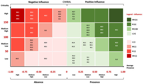
Figure 10.
Matrix of Influence With 53 Categories (CIMBAL). Source: the authors.
The “cloud” on the left and, in particular, the top left, is notorious, with three categories from the Decision stage having a Very High and Negative influence: D4.1, D3.2 and D4.4. As the matrix shows, numerous categories of the Decision stage had a negative or very negative influence on the CIMBAL case. It is also worth mentioning the fact that several categories of the Agenda stage had a high and positive influence. In this matrix, we have 30 categories with a positive influence and 23 with a negative influence (those with, respectively, PM > 0 and PM < 0). Table 8 shows the distribution by level of influence.
Table 8.
Number of Categories by Level of Influence (CIMBAL).
In Figure 11, we can see the distribution of categories in the CIMVDL case. The differences are immediately visible. In this case, the spot is on the right side with a large presence of categories at the top right with nine categories with very high influence and twenty-nine with high influence. It should be noted that in the set of nine categories with very high (and positive) influences, we have an equitable distribution across the three stages:
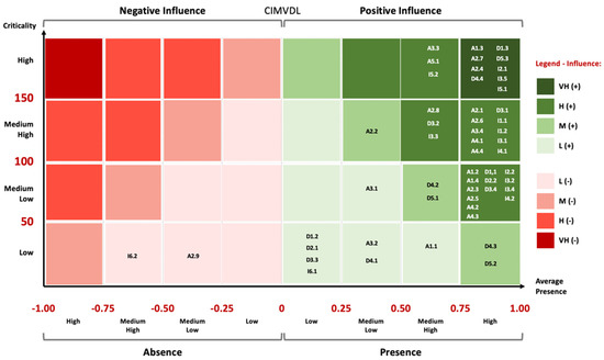
Figure 11.
Matrix of Influence with 53 Categories (CIMVDL). Source: the authors.
- Agenda: A1.3, A2.4 and A2.7
- Decision: D1.3, D4.4 and D5.3
- Implementation: I2.1, I3.5 and I5.1
In this matrix, we have fifty-one categories with a positive influence and two with a negative influence (those with, respectively, AP > 0 and AP < 0). Table 9 shows the distribution by level of influence.
Table 9.
Number of Categories by Level of Influence (CIMVDL). Source: the authors.
5. Conclusions
5.1. Discussion: Articulation of the Proposed Methodology with the Identification of Explaining Factors of the Public Policy Cycle under Analysis
The previous sections presented and analysed the effects of the actions and activities carried out by the different decision makers and agents involved throughout the public policy cycle in the two Portuguese Intermunicipal Communities. Given the specificity of the approach for Intermunicipal cases, we sought to understand, for each stage and in a comparative way, which are the differentiating success/failure factors between the two realities, as well as which ones were less influential.
Effectively, it was possible to verify according to the theory [59] that the analysis of data obtained based on the semi-structured interviews carried out turned out to be a very complex part of our interpretive research work. We carried out our work based on authors specialized in research methods [12,37], as well as on the consultation of works in qualitative [8,18] and quantitative [1] research. This ensured that the data analysis performed was conducted in a rigorous and methodical way and the path we took presented significant and useful results.
Indeed, figures and tables presented and the respective Matrices of Influence for each case pose in a systematized and contrasted way what were the most differentiating factors in the process of scheduling, decision and implementation of EEP. This contributes to a broader knowledge regarding the explanation of the two cases under study. The comparative analysis of the two cases made it possible to verify, demonstrate and identify the factors that make the CIMVDL a case of success and CIMBAL a case of failure when it came to public policy on EEP in those territories. Effectively, the approach presented may be replicated by researchers intending to address similar cases related to public or corporate policies and decisions and understand in a systematic, traceable, transparent and less impressionistic/subjective way how issues developed and what actions/behaviours were critical for the success or failure. Therefore, the methodology that we presented and that enabled this process allowed us to answer our initial research question, on how we could extract, organize and communicate insights from a vast amount of qualitative information. Through the measurement tools, indexes and matrices of influence presented, we were able not only to systematize information, but also to ascertain concrete conclusions and present them in a visual way. This made clearer the implications, concepts and dynamics underlying qualitative analysis, with the ultimate goal of facilitating the understanding of the phenomenon under study according to suggestions proposed in previous works [33,48,58].
5.2. Limitations
Content analysis is inherently a qualitative analysis and it is characterized by a particular and unsurpassable subjectivity [60]. The fact that the extent of the work developed (number and extension of the quotes selected in the transcript of the 39 interviews) did not allow time for other researchers to be asked to carry out a similar qualitative content analysis can be seen as a limitation. Especially with regard to the allocation of each quote to the category of the theoretical model adopted or the corresponding classification of the type of effect inherent to CISF. However, we believe that the coding and classification rules adopted—clearly and consistently applied throughout the analysis—allow us to envision that different researchers would reach similar results if they categorised the same contents based on these rules.
A second limitation is linked to lack of quantitative data on the phenomenon studied based on the processing of data from questionnaires, structured interviews, measurement scales or standardised tests (e.g., satisfaction surveys about the programs, test results of students involved in the programs, specific quantitative studies on programs carried out). This does not enable the (possible) adoption of the triangulation strategy, i.e., the use of different combined methods in order to increase the reliability of the data and the conclusions explored by the authors within the scope of the study. Both limitations—the second, in particular—are aligned with the suggestions presented as possible extensions of this work.
5.3. Contribution to Mixed Methods Research, Social Sciences and Mathematics
This work presents a carefully constructed structure that portrays the phases of qualitative and quantitative analysis of the content of the interviews carried out based on accepted scientific approaches in the treatment of qualitative and quantitative data. Contrary to the tendency of qualitative researchers [61] when arguing on the basis of quantitative logic (e.g., “5 of the respondents said”, “most of the answers focused”), the work carried out allowed an interpretation and presentation of theoretically grounded results.
Indeed, we chose to build a model that could handle the 3749 quotes gathered in the interviews, so as not to limit ourselves to a purely qualitative type of study that would necessarily lead to simple impressions taken from the interviews. Even if it was a more arduous and complex path, the study carried out, as mentioned in this paper, adopted a mixed methods approach, predominantly qualitative, insofar as the quantitative analysis does not result from the direct collection of quantitative data, but from the quantification of qualitative data. The difference for a qualitative study only is, however, absolutely colossal. It is enough to mention that to order the 53 categories of the model without resorting to quantitative tools, the researcher would have to, through his “memories” and “impressions”, try to compare 1378 pairs of categories (combinations of 53 in pairs = 53C2 = (53 × 52)/2 = 1378).
Given the complexity of the phenomenon studied, and in addition to the methodological strategy followed in the qualitative variant, we resorted to different approaches to the notion of measure to guarantee the operations carried out since the way in which concepts are defined and measured has a direct influence on the validity of research results and, therefore, on the theoretical validity of the study [12]. To that end, a process of operationalization of the concepts was followed, inspired by the five steps proposed by Fortin [12], i.e., (i) precision of the conceptual definitions; (ii) specification of the dimensions of the concept; (iii) empirical indicators; (iv) measurement operations. In this process, we paid special attention to the prior definition of the object of analysis that was intended to be quantified; the elaboration of appropriate instruments to carry out the measurement operation and respective scale; the systematic construction of indicators, indexes and rankings; finally, the creation of a matrix of influence as a facilitating instrument for reading and presenting the results.
Regarding steps (i) and (ii), we highlight the creation of two absolutely critical “intermediate” variables—the CISFs and their type of effect—and TEICC. Both are “intermediate” variables in that they were essential to bridge the gap between the theoretical framework adopted and the quantitative analysis of qualitative data. After coding, we were faced with the challenge of attributing a qualitative label and then attributing a score to each label. The step of attributing a label required the creation of a new concept—the CISF. Without it, we simply could not “connect” the quotes to the descriptions in the theoretical models adopted. The attribution of a score further required that we created a new “unit of measure”, the TEICC (“type of effect implicit in the coded citation”). Only with this could we evaluate the presence/absence of the CISF and its type of magnitude/impact (high or low). These resulted, respectively, in the creation of four types of effects implicit in the selected quote (B, R, E or D) and its quantification (−1, −0.5, 0.5 and 1, respectively). These are key foundations that allowed us to build the indicators that would support and feed the final matrix of influence where we plot all the categories.
Thus, the standardisation carried out was essential to treat the empirical elements collected and extract value from them. In fact, without this standardisation, the difficulties of interpretation and comparison between the elements of the three selected models (Kindgon’s, Lindblom’s and Sabatier and Mazmanian’s)—and given a sample of 3749 citations—would be enormous.
We characterize this work as a methodological contribution insofar as the identification and detailed description of all the research steps related to the qualitative and quantitative treatment of the data seem to us to be relevant for future works. The systematic and transparent approach was adopted with a detailed description of the methodological aspects related to the quantification of qualitative data—including, among others, the definition of concepts, constructs, types of measure and the entire process of construction of indicators—allows us to add it to qualitative outputs.
5.4. Future Research
Although it is possible to see, in the literature, repeated attempts to quantify statements from open interviews or narratives [62,63], the statements are usually analysed only in terms of frequencies (which allows specification and some terms of comparison). We acted in harmony with this theoretical premise through the counting of frequencies by category, stage and the theoretical model adopted—which allowed a snapshot of the relevance of the different constitutive elements of the conceptual model adopted. However, even though the frequency count—the number of quotes allocated to a given category—allows the identification of the most outstanding categories (on the assumption that the more quotes a category has, the more relevant that category will be research-wise), that alone was not enough to understand to what extent the presence (or absence) of some elements contributed (or not) to the success in each of the stages of the policy cycle. Our study wanted to go beyond this and answer more questions. The instruments developed to ascertain the type and intensity of the impact of the various elements may inspire the adoption of new procedures or adaptation of protocols in the quantitative treatment of qualitative data. Future researchers who intend to measure some of the elements that contribute to the understanding of a given phenomenon, in different areas of knowledge requiring the use of data collection techniques supported by semi-structured interviews or open, may find new tools to do so.
A possible extension of this study would be based on the theoretical model adopted, as well as on the indicators and indexes created. The formulation of standardised surveys that could be adopted and sent to different actors involved in a similar situation in the fields of social, political and economic sciences is something that can be carried out. With this typology of surveys, it would then be possible to directly question these actors what values they would attribute, given a pre-defined scale, to the presence and magnitude of the variables contained in the corresponding surveys. In fact, the adoption of this data collection method could allow interviewees to directly assign a score (on a certain scale) to the presence and magnitude of the CISFs, instead of a researcher that needed to choose, code and classify a given quote. This would, of course, be a work with a strong quantitative dimension, in which subjectivity would be even more mitigated. This would also enable a more extensive statistical treatment based on approaches already established in the literature.
Furthermore, the treatment of data and all the research steps presented may encourage future works in which teams of researchers have to deal with vast amounts of qualitative data and may find helpful a quantitization process that reduces subjectivity (which would address the first limitation mentioned above). The outcomes of the process we propose can then be cross-checked with the results from methods used by researchers that carried out purely qualitative analyses. The use and analysis of semi-structured interviews can, thus, acquire new breadth. This would be particularly relevant in the fields of public policy studies and other social sciences that deal with conceptual frameworks in combination with methods that privilege the gathering of qualitative inputs.
Finally, given that right now no software can analyse qualitative data [64]—only help in the analysis process—our proposal may also resonate in research on artificial intelligence, i.e., AI could be developed to find ways to process some steps of the process digitally. This way, sample sizes would not be as time-consuming as they are now, and human intervention would be reduced to the least necessary amount. This would allow researchers to attain results faster and in a more efficient way. Indeed, the use of Computer Assisted Qualitative Data Analysis Software (as is the case of NVIVO, which we had the chance to use and proved fruitful, as we have demonstrated at an earlier stage of this paper) is useful and helps produce results with increased transparency, traceability and methodological rigour when large amounts of data are involved.
5.5. Final Remarks
In this paper, we explored a concrete application of quantitizing qualitative data from semi-structured interviews—a mixed methods approach in the context of a social sciences study. Through the quantitizing process we were able to extract more information from the interviews, reducing subjectivity and presenting the main results in a more comprehensive, organized and structured manner, highlighting two key dimensions of the subject being studied (degree of “criticality” and “presence” of the CISF), summarised in a matrix of influence. As for the specific case study used to illustrate our methodology, the process, which culminated in the matrices of influence, led to the identification, per stage of the public policy cycle, of which factors determined the success (or lack thereof) of the implementation of EEP in Portugal. Namely, the rationale behind the reasons why decision makers decided to implement EEP in CIMVDL and not in CIMBAL. If readers want more context, outside the scope of this paper, they can check our recent study [65]. As Figure 9 explained, the AP, FCI, AM, IF and IAM indicators were crucial to ascertain the IC and IAP, which, in turn, led to the construction of the Matrix of Influence and the readability of results.
The transparent and systematic approach adopted—including a clear definition of concepts, constructs, measurement tools and a traceable process of construction of indicators—allowed us to obtain a broader knowledge of the phenomenon under study than if we had only adopted a qualitative approach to address the content of the interviews made [46]. Moreover, given the transparency and (relative) objectivity of the process, we believe other researchers doing the same work would achieve similar results.
Therefore, we believe that this methodological approach, which comprises a variety of steps and theoretically based choices, may not only be of interest to social scientists seeking to bring new dimension to their studies, but also contribute to the overall research based on the combination of qualitative and quantitative methods to perform a content analysis of data from the processing of semi-structured interviews.
Supplementary Materials
The following supporting information can be downloaded at: https://www.mdpi.com/article/10.3390/math10193597/s1. Ref. [39] has been cited in supplementary materials.
Author Contributions
Writing—original draft, F.B., A.F. and L.S.C. All authors have read and agreed to the published version of the manuscript.
Funding
This research received no external funding.
Conflicts of Interest
The authors declare no conflict of interest.
References
- Sandelowski, M.; Voils, C.I.; Knafl, G. On Quantitizing. J. Mix. Methods Res. 2009, 3, 208–222. [Google Scholar] [CrossRef] [PubMed]
- Bryman, A.; Bell, E. Business Research Methods; Oxford University Press: Oxford, UK, 2015. [Google Scholar]
- Lincoln, Y.S.; Guba, E. Naturalistic Inquiry; Sage: Beverly Hills, CA, USA, 1985. [Google Scholar]
- Gummesson, E. Qualitative Research Methods in Management Research; Sage: Thousand Oaks, CA, USA, 2000. [Google Scholar]
- Remenyi, A.; Good, M.C.; Bhattacharyya, R.P.; Lim, W.A. The Role of Docking Interactions in Mediating Signaling Input, Output, and Discrimination in the Yeast MAPK Network. Mol. Cell 2005, 20, 951–962. [Google Scholar] [CrossRef] [PubMed]
- Flick, U. Métodos Qualitativos na Investigação Científica; Monitor: Lisbon, Portugal, 2005. [Google Scholar]
- Tashakkorí, A.; Teddlie, C. (Eds.) Handbook of Mixed Methods in the Social and Behavioral Sciences; Sage: Thousand Oaks, CA, USA, 2003. [Google Scholar]
- Gale, N.K.; Heath, G.; Cameron, E. Using the framework method for the analysis of qualitative data in multi-disciplinary health research. BMC Med. Res. Methodol. 2013, 13, 117. [Google Scholar] [CrossRef] [PubMed]
- Denzin, N.; Lincoln, Y. Introduction: The discipline and practice of qualitative research. In The Sage Handbook of Qualitative Research; Denzin, N., Lincoln, Y., Eds.; Sage: Thousand Oaks, CA, USA, 2011. [Google Scholar]
- Tomaszewski, L.E.; Zarestky, J.; Gonzalez, E. Planning Qualitative Research: Design and Decision Making for New Researchers. Int. J. Qual. Methods 2020, 19, 1609406920967174. [Google Scholar] [CrossRef]
- Creswell, J.; Poth, C. Qualitative Inquiry and Research Design: Choosing Among Five Approaches; Sage: Los Angeles, CA, USA, 2018. [Google Scholar]
- Fortin, M. O Processo de Investigação: Da Conceção à Realização; Lusociência-Edições: Lisbon, Portugal, 2009. [Google Scholar]
- Nushi, M.; Momeni, A.; Roshanbin, M. Characteristics of an Effective University Professor From Students’ Perspective: Are the Qualities Changing? Front. Educ. 2022, 7, 842640. [Google Scholar] [CrossRef]
- Dewasiri, N.J.; Weerakoon, Y.K.B. Why do companies pay dividends? A comment. J. Corp. Ownersh. Control 2016, 13, 443–453. [Google Scholar] [CrossRef]
- Borgstede, M.; Scholz, M. Quantitative and Qualitative Approaches to Generalization and Replication: A Representationalist View. Front. Psychol. 2021, 12, 605191. [Google Scholar] [CrossRef]
- Creswell, J.W. Research Design—Qualitative, Quantitative, and Mixed Methods Approaches; Sage: Los Angeles, CA, USA, 2009. [Google Scholar]
- Maguire, M.; Delahunt, B. Doing a Thematic Analysis: A Practical, Step-by-Step Guide for Learning and Teaching Scholars. AISHE-J. 2017; 9, 3. [Google Scholar]
- Nowell, L.S.; Norris, J.M.; White, D.E.; Moules, N.J. Thematic Analysis: Striving to Meet the Trustworthiness Criteria. Int. J. Qual. Methods 2017, 16, 1609406917733847. [Google Scholar] [CrossRef]
- Costa, K. Systematic Guide to Qualitative Data Analysis Within the C.O.S.T.A. Postgraduate Research Model. OSF Prepr. 2019. [Google Scholar] [CrossRef]
- Wolcott, H.F. Transforming Qualitative Data: Description, Analysis, and Interpretation; Sage: Thousand Oaks, CA, USA, 1994. [Google Scholar]
- Boyatzis, R.E. Transforming Qualitative Information: Thematic Analysis and Code Development; Sage: Thousand Oaks, CA, USA, 1998. [Google Scholar]
- Driscoll, D.L.; Appiah-Yeboah, A.; Salib, P.; Rupert, D.J. Merging qualitative and quantitative data in mixed methods research: How to and why not. Ecol. Environ. Anthropol. 2007, 3, 1. [Google Scholar]
- Sandelowski, M. Real qualitative researchers do not count: The use of numbers in qualitative research. Res. Nurs. Health 2001, 24, 230–240. [Google Scholar] [CrossRef] [PubMed]
- Braun, V.; Clarke, V. Using thematic analysis in psychology. Qual. Res. Psychol. 2006, 3, 77–101. [Google Scholar] [CrossRef]
- Weis, D.; Willems, H. Aggregation, Validation, and Generalization of Qualitative Data—Methodological and Practical Research Strategies Illustrated by the Research Process of an empirically Based Typology. Integr. Psychol. Behav. 2017, 51, 223–243. [Google Scholar] [CrossRef] [PubMed]
- Guetterman, T.C.; Fetters, M.D.; Creswell, J.W. Integrating Quantitative and Qualitative Results in Health Science. Mixed Methods Research Through Joint Displays. Ann. Fam. Med. 2015, 13, 554–561. [Google Scholar] [CrossRef]
- Elliott, V. Thinking about the Coding Process in Qualitative Data Analysis. Qual. Rep. 2018, 23, 2850–2861. [Google Scholar] [CrossRef]
- Johnson, R.; Onwuegbuzie, A.J. Mixed Methods Research: A Research Paradigm Whose Time Has Come. Educ. Res. 2004, 33, 14–26. [Google Scholar] [CrossRef]
- Harris, L.R.; Brown, G.T.L. Mixing interview and questionnaire methods: Practical problems in aligning data. Pract. Assess. Res. Eval. 2010, 15, 1. [Google Scholar]
- Bogdan, R.; Biklen, S.K. Investigação Qualitativa em Educação; Porto Editora: Porto, Portugal, 1994. [Google Scholar]
- Olabuénaga, J.I.R. Metodología de la Investigación Cualitativa; Universidad de Deusto: Bilbao, Spain, 2003. [Google Scholar]
- Säumel, I.; Reddy, S.; Wachtel, T.; Schlecht, M.; Ramos-Jiliberto, R. How to feed the cities? Co-creating inclusive, healthy and sustainable city region food systems. Front. Sustain. Food Syst. 2022, 6. [Google Scholar] [CrossRef]
- Lofland, J.; Snow, D.A.; Anderson, L.; Lofland, L.H. Analyzing Social Settings, A Guide To Qualitative Observation And Analysis; Belmont: Wadsworth, OH, USA, 2006. [Google Scholar]
- Merriam, S.B. Qualitative Research and Case Study Applications in Education; Jossey-Bass Publishers: San Francisco, CA, USA, 1998. [Google Scholar]
- Demazière, D.; Dubar, C. Analyser Les Entretiens Biographiques: L’exemple De Récits D’insertion; Nathan: Paris, France, 1997. [Google Scholar]
- Ruquoy, D. Situação de Entrevista e Estratégia do Entrevistador. In Práticas e Métodos de Investigação em Ciências Sociais (84-117); Albarello, L., Digneffe, F., Hiernaux, J.-P., Maroy, C., Ruquoy, D., Saint-Georges, P., Eds.; Gradiva: Lisbon, Portugal, 1997. [Google Scholar]
- Miles, M.B.; Huberman, A.M.; Saldana, J. Qualitative Data Analysis: An Expanded Sourcebook; Sage: Thousand Oaks, CA, USA, 2018. [Google Scholar]
- Howlett, M.; Ramesh, M.; Perl, A. Studying public policy: Principles and Processes; Oxford University Press: Oxford, UK, 2020. [Google Scholar]
- Banha, F.; Flores, A.; Coelho, L.S. A New Conceptual Framework and Approach to Decision Making in Public Policy. Knowledge 2022, 2, 539–556. [Google Scholar] [CrossRef]
- Kingdon, J.W. Agendas, Alternatives and Public Policies; Little Brown: Boston, MA, USA, 1984. [Google Scholar]
- Lindblom, C.E. The Science of “Muddling Through”. Public Adm. Rev. 1959, 19, 79–88. [Google Scholar] [CrossRef]
- Lindblom, C.E. Still muddling, not yet through. Public Adm. Rev. 1979, 39, 517–526. [Google Scholar] [CrossRef]
- Sabatier, P.A.; Mazmanian, D.A. The Implementation of Public Policy: A Framework of Analysis. Policy Stud. J. 1980, 8, 538–560. [Google Scholar] [CrossRef]
- Banha, F. Implementação de Programas de Educação Para o Empreendedorismo: Processos de Decisão no Caso Português. Ph.D. Thesis, University of Algarve, Faro, Portugal, 2020. Available online: https://sapientia.ualg.pt/handle/10400.1/15239 (accessed on 3 June 2022).
- Bardin, L. Análise de Conteúdo; Edições 70: Lisbon, Portugal, 2018. [Google Scholar]
- Mayring, P. Qualitative Content Analysis. Forum. Qual. Soc. Res. 2000, 1, 159–176. [Google Scholar]
- Flick, U. The SAGE Handbook of Qualitative Data Analysis; Sage: Los Angeles, CA, USA, 2013. [Google Scholar]
- Miles, M.B.; Huberman, A.M. Qualitative Data Analysis: A Sourcebook of New Methods; Sage: Thousand Oaks, CA, USA, 1984. [Google Scholar]
- Fawcett, J.; Downs, F. The Relationship of Theory and Practice; F A Davis: Philadelphia, PA, USA, 1992. [Google Scholar]
- Quivy, R.; Campenhoudt, L.V. Manual de investigação em ciências sociais. In Contributo para otimizar a Gestão de Recursos Humanos nas Secções de Recursos Logísticos e Financeiros da Guarda Nacional Republicana: A Importância da Formação em Contratação pública; Gradiva: Lisbon, Portugal, 2017. [Google Scholar]
- Bhandari, P. Operationalization|A Guide with Examples, Pros & Cons. Scribbr. 2022. Available online: https://www.scribbr.com/methodology/operationalization/ (accessed on 2 August 2022).
- Krippendorff, K. Content analysis: An Introduction to its Methodology; Sage: Thousand Oaks, CA, USA, 2004. [Google Scholar]
- Saldaña, J. The Coding Manual for Qualitative Researchers; Sage: Thousand Oaks, CA, USA, 2013. [Google Scholar]
- Trzesniak, P. Indicadores Quantitativos: Reflexões que Antecedem seu Estabelecimento. Ciência Da Inf. 1998, 27, 159–164. [Google Scholar] [CrossRef][Green Version]
- Greco, S.; Ishizaka, A.; Tasiou, M.; Torrisi, G. On the Methodological Framework of Composite Indices: A Review of the Issues of Weighting, Aggregation, and Robustness. Soc. Indic. Res. 2019, 141, 61–94. [Google Scholar] [CrossRef]
- Jannuzzi, G. Indicadores Sociais na Formulação e Avaliação de Políticas Públicas. Rev. Bras. De Adm. Pública 2002, 36, 51–72. [Google Scholar]
- OECD. Handbook on Constructing Composite Indicators; OECD: Paris, France, 2008. [Google Scholar]
- Verdinelli, S.; Scagnoli, N.I. Data display in qualitative research. Int. J. Qual. Methods 2013, 12, 359–381. [Google Scholar] [CrossRef]
- Thorne, S. Data Analysis in Qualitative Research. Evid. Based Nurning 2000, 3, 14. [Google Scholar] [CrossRef]
- Graneheim, U.; Lundman, B. Qualitative Content Analysis in Nursing Research: Concepts, Procedures and Measures to Achieve Trustworthiness. Nurse Educ. Today 2003, 24, 105–112. [Google Scholar] [CrossRef]
- Hopf, C. Norm und Interpretation. Z. Fur Soziologie 1982, 11, 307–329. [Google Scholar] [CrossRef]
- Mühlfeld, C.; Windolf, P.; Lampert, N.; Krüger, H. Auswertungsprobleme Offener Interviews. Soziale Welt 1981, 32, 325–352. [Google Scholar]
- Engel, U.; Wuggenig, U. Statistische Auswertungsverfahren nominalskalierter Daten. In Handbuch Qualitative Sozialforschung; Flick, U., Von Kardorff, E., Keupp, L., Von Rosenstiel, L., Wolff, S., Eds.; Psycholgie Verlags Union: München, Germany, 1995. [Google Scholar]
- Zamawe, F.C. The Implication of Using NVivo Software in Qualitative Data Analysis: Evidence-Based Reflections. Malawi Med. J. 2015, 27, 13–15. [Google Scholar] [CrossRef] [PubMed]
- Banha, F.; Flores, A.; Coelho, L.S. NUTS III as Decision-Making Vehicles for Diffusion and Implementation of Education for Entrepreneurship Programmes in the European Union: Some Lessons from the Portuguese Case. Educ. Sci. 2022, 12, 436. [Google Scholar] [CrossRef]
Publisher’s Note: MDPI stays neutral with regard to jurisdictional claims in published maps and institutional affiliations. |
© 2022 by the authors. Licensee MDPI, Basel, Switzerland. This article is an open access article distributed under the terms and conditions of the Creative Commons Attribution (CC BY) license (https://creativecommons.org/licenses/by/4.0/).