Development and Research of a Modified Upwind Leapfrog Scheme for Solving Transport Problems

Abstract

Modeling complex hydrodynamic processes in coastal systems is an important problem of mathematical modeling that cannot be solved analytically. The approximation of convective terms is difficult from the point of view of error reduction. This paper proposes a difference scheme based on a linear combination of the Upwind Leapfrog scheme with 2/3 weight coefficient, and the Standard Leapfrog scheme with 1/3 weight coefficient. The weight coefficients are obtained as a result of solving the problem of minimizing the approximation error. Numerical experiments show the advantage of the developed scheme in comparison with other modifications of the Upwind Leapfrog scheme in the case when the convective transport prevails over the diffusion one. The proposed difference scheme solves transport problems more effectively than classical difference schemes in the case when the Péclet number falls in the range from 2 to 20. It follows that the considered difference scheme allows hydrodynamic problems to be solved in regions of complex shape effectively.

1. Introduction

Solving problems of hydrodynamics is an important field of science that allows for the modeling and forecasting of adverse and dangerous natural and anthropogenic phenomena in coastal systems. Examples include run-up phenomena under wind influences, the spread of pollutants, including oil and petroleum products, blooming waters, and the mass death of commercial fish species due to a lack or absence of dissolved oxygen. The problem of modeling unsteady transport processes in a three-dimensional domain of complex shape cannot be solved analytically, and requires the use of numerical methods [1,2,3]. At work [4], the finite volume method on structured non-uniform grids for 1D and 2D shallow water equations is considered.The paper [5] presents a solution to a two-dimensional non-stationary convection–diffusion problem using the boundary element method of radial integration. This algorithm requires only boundary discretization and some internal points, instead of internal cells. The proposed method accuracy and efficiency are researched in this work. Adaptive iterative splitting methods to solve convection–diffusion–reaction problems is proposed in paper [6]. Adaptive techniques are embedded into the splitting approach, when developing this method. The paper [7] presents an upwind difference scheme for interface flux approximations for the finite volume method. The upwind approach is proposed for spatial interface approximation, and the second-order formulation is used for the temporal approximation in this work. The finite volume method on unstructured grids is proposed for transport problems in which convection dominates diffusion [8]. The research [9] considers a high-order finite volume complete flux scheme for a one-dimensional advection–diffusion–reaction equation. In this work, the accuracy increases to the fourth order due to applying Gauss–Legendre quadrature rules to the integral representation. The presented scheme works for both diffusion dominated and advection dominated flow.

A number of papers present reviews and developments of various numerical approaches to linear [10,11,12,13,14,15] and nonlinear [11,13,15] transport, and convection–diffusion problems, as applied to finite element methods and finite difference methods. In the numerical solution of the transport problem, a problem related to the insufficient accuracy of the approximation of convective terms arises. The specialized difference schemes for solving convection–diffusion problems were developed and described in [16]. Upwind Leapfrog schemes were used to solve aeroacoustics problems [17,18]. The monotonicity of difference schemes is researched in [19,20,21], including the Upwind Leapfrog schemes for the transport problem. A number of papers were devoted to the consideration of various modifications of the Upwind Leapfrog scheme, including [22], in which it was proposed to use weight multipliers to eliminate oscillations when solving a nonlinear transport problem. To solve this class of problems, a difference scheme was proposed, which is a linear combination of Standard Leapfrog and Upwind Leapfrog schemes [23]. The considered schemes are included in a linear combination with weight coefficients of 1/3 and 2/3, respectively, which are obtained from the solution of minimizing the order of the approximation error problem [24].

A linear combination of two schemes with similar properties often has better properties than the original schemes, since there is a mutual compensation of approximation errors. The purpose of this work is to determine the range of the grid Péclet number values, in which the proposed scheme, which is a linear combination of the Upwind Leapfrog scheme with 2/3 weight coefficient, and Standard Leapfrog scheme with 1/3 weight coefficient, obtained as a result of solving the problem of minimizing the approximation error, has better accuracy compared to classical schemes, including modifications of the Upwind Leapfrog scheme with limiters. Solutions of test problems of transport in areas of complex shape using the developed scheme are considered in the work [25]. These are problems such as the test problem of the fluid flow between two coaxial circular cylinders at different grid Péclet numbers, and the problem of suspended particles transport during soil dumping in areas with complex geometry. An application of this scheme to solve the problem with nonlinear dispersion wave equations is described by the model Korteweg–de Vries equation considered in [26]. The advantage of the presented difference scheme in comparison with the standard ones in problems with the predominance of convective transport over diffusion is shown.

The article is devoted to the construction and study of a difference scheme, which is a linear combination of the Upwind and Standard Leapfrog schemes. Section 2 discusses the classical schemes of Upwind and Standard Leapfrog through the example of solving the transport problem. Section 3 describes the proposed scheme based on a linear combination of Upwind and Standard Leapfrog schemes. In Section 4, the results of solving a test problem based on the considered scheme are compared with other modifications of the Upwind and Standard Leapfrog schemes. In Section 5 and Section 6, the accuracy of solving the model diffusion–convection problem based on the proposed scheme is investigated for different values of the Péclet grid number. In Conclusions, an analysis of the results obtained in the work is given.

2. Upwind and Standard Leapfrog Difference Schemes for the Transport Equation

Consider the transport equation:

$$\frac{\partial q}{\partial t}+u\frac{\partial q}{\partial x}=0,$$

(1)

where $t\in \left[0,T\right]$, $x\in \left[0,L\right]$, $q\left(0,x\right)=q^0\left(x\right)$, $q\left(t,0\right)=0$ if $u\ge 0$, and $q\left(t,L\right)=0$ if $u<0$, $u=const$.

A uniform computational grid is introduced:

$$\omega ={\overline{\omega }}_h\times {\omega }_{\tau },$$

(2)

where ${\overline{\omega }}_h=\left\{\left.x_i\right|x_i=ih,i=\overline{0,N_x},N_{x}h=L\right\}$, and where $h=x_{i+1}-x_i=const$ is the space step; $N_x$ is the number of nodes in space; L is the characteristic dimension of the computational domain, ${\omega }_{\tau }=\left\{\left.t^n\right|t^n=n\tau ,n=\overline{0,N_t},N_t\tau =T\right\}$, where $\tau =t^{n+1}-t^n=const$ is the time step; $N_t$ is the number of time layers; T is the upper bound in time.

The following finite-difference schemes can be used for the numerical solution of the problem (1):

• The Upwind Leapfrog scheme:

  $$\begin{array}{c}\hfill \frac{q_i^{n+1}-q_i^n}{2\tau }+\frac{q_{i-1}^n-q_{i-1}^{n-1}}{2\tau }+u\frac{q_i^n-q_{i-1}^n}{h}=0,u\ge 0;\\ \hfill \frac{q_i^{n+1}-q_i^n}{2\tau }+\frac{q_{i+1}^n-q_{i+1}^{n-1}}{2\tau }+u\frac{q_{i+1}^n-q_i^n}{h}=0,u<0,\end{array}$$

  (3)

  where $q_i^n=q\left(t^n,x_i\right)$, $q_i^{n+1}=q\left(t^{n+1},x_i\right)$, $q_{i\pm 1}^n=q\left(t^n,x_{i\pm 1}\right)$, $q_{i\pm 1}^{n-1}=q\left(t^{n-1},x_{i\pm 1}\right)$.
• The Standard Leapfrog scheme:

  $$\frac{q_i^{n+1}-q_i^{n-1}}{2\tau }+u\frac{q_{i+1}^n-q_{i-1}^n}{2h}=0.$$

  (4)

Test problem I. Find the solution to the equation:

$$\frac{\partial q}{\partial t}+u\frac{\partial q}{\partial x}=0,u=0.5\mathrm{m}/\mathrm{s},0\le t\le T,0\le x\le L,q\left(t,0\right)=0,$$

with initial distribution $q^0\left(x\right)=\theta (20-x)-\theta (10-x)$, where $\theta \left(x\right)$ is the Heaviside function.

For the numerical solution of the problem, we introduce a uniform computational grid:

Parameters of the calculation grid: time step $\tau =0.02$ s, space step $h=1$ m, the length of the time interval $T=100$ s, the length of the space interval $L=100$ m.

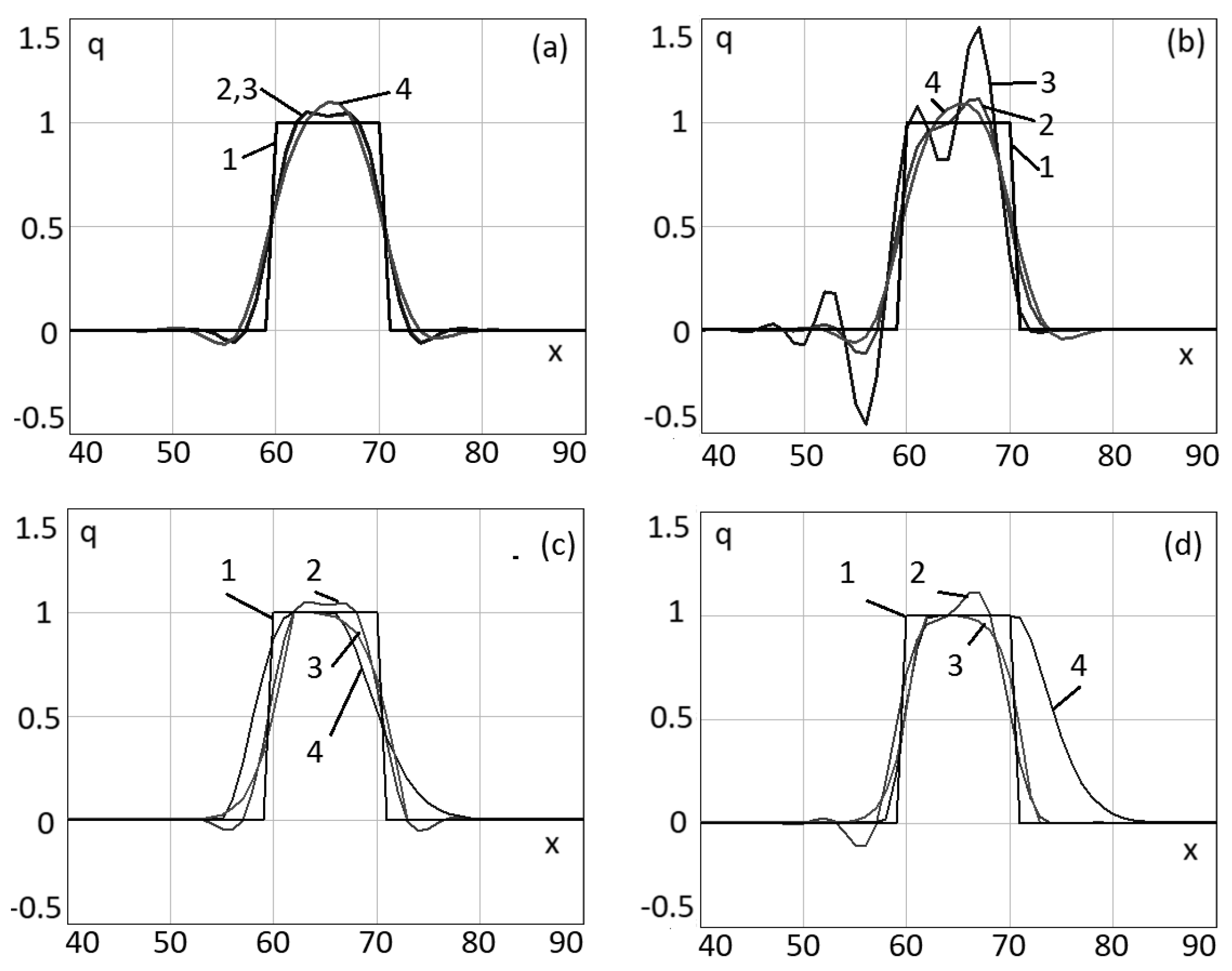
Figure 1 shows the exact solution of the test problem I, and numerical solutions based on the difference schemes (3) and (4), the Upwind Leapfrog difference scheme with TVD-limiters, and the Standard Leapfrog difference scheme with TVD-limiters [27].

Comment 1.Figure 1a,b show that the solutions of test problem I based on difference schemes (3) and (4) have dispersion-induced oscillations in front of the leading and trailing fronts of the wave, respectively. We also note that for the solution based on the difference scheme (3), high harmonics have a “phase velocity” that is higher than the real one, and for the solution based on the scheme (4), it is lower.

Comment 2. Difference schemes (3) and (4), due to their non-dissipativity and non-monotonicity, are not recommended for solving transport problems in the case of discontinuous initial data. Their application to such problems is possible by implementing procedures that monotonize the solution; for example, by adding artificial viscosity. For scheme (3), it is recommended to use a non-linear flow correction (TVD-limiters) [27] based on the maximum principle. Figure 1c,d present the solutions of the test problem I based on the Upwind and Standard Leapfrog schemes with TVD-limiters [27]. Note that the difference scheme obtained as a result of a linear combination of the Upwind Leapfrog [27] and Standard Leapfrog schemes is no longer dissipative, but the dispersion properties of the scheme can be improved and the solution obtained based on a combination of difference schemes on discontinuous functions may have smaller oscillations.

3. Linear Combination of Upwind and Standard Leapfrog Schemes

Consider the Upwind Leapfrog difference scheme (3) (the case $u\ge 0$). Let’s use the decomposition of the functions $q_i^{n\pm 1}$ in the Taylor series in the node $\left(i,n\right)$ neighborhood:

$$q_i^{n\pm 1}=q_i^n\pm \tau {\left(\frac{\partial q}{\partial t}\right)}_i^n+\frac{{\tau }^2}{2}{\left(\frac{{\partial }^{2}q}{{\partial t}^2}\right)}_i^n\pm \frac{{\tau }^3}{3!}{\left(\frac{{\partial }^{3}q}{{\partial t}^3}\right)}_i^n+\frac{{\tau }^4}{4!}{\left(\frac{{\partial }^{4}q}{{\partial t}^4}\right)}_i^n+O\left({\tau }^5\right).$$

(5)

Let’s use the decomposition of the functions $q_{i-1}^n$ and $q_i^n$ in the Taylor series in the node $\left(i-1/2,n\right)$ neighborhood:

$$\begin{array}{c}\hfill q_{i-1}^n=q_{i-1/2}^n-\frac{h}{2}{\left(\frac{\partial q}{\partial x}\right)}_{i-1/2}^n+\frac{h^2}{8}{\left(\frac{{\partial }^{2}q}{{\partial x}^2}\right)}_{i-1/2}^n-\frac{h^3}{48}{\left(\frac{{\partial }^{3}q}{{\partial x}^3}\right)}_{i-1/2}^n+\\ \hfill +\frac{h^4}{384}{\left(\frac{{\partial }^{4}q}{{\partial x}^4}\right)}_{i-1/2}^n+O\left(h^5\right);\end{array}$$

(6)

$$\begin{array}{c}\hfill q_i^n=q_{i-1/2}^n+\frac{h}{2}{\left(\frac{\partial q}{\partial x}\right)}_{i-1/2}^n+\frac{h^2}{8}{\left(\frac{{\partial }^{2}q}{{\partial x}^2}\right)}_{i-1/2}^n+\frac{h^3}{48}{\left(\frac{{\partial }^{3}q}{{\partial x}^3}\right)}_{i-1/2}^n+\\ \hfill +\frac{h^4}{384}{\left(\frac{{\partial }^{4}q}{{\partial x}^4}\right)}_{i-1/2}^n+O\left(h^5\right).\end{array}$$

(7)

Taking into account the scheme (1), we have:

$$\frac{\partial q}{\partial t}=-u\frac{\partial q}{\partial x},\frac{{\partial }^{2}q}{{\partial t}^2}=u^2\frac{{\partial }^{2}q}{{\partial x}^2},\frac{{\partial }^{3}q}{{\partial t}^3}=-u^3\frac{{\partial }^{3}q}{{\partial x}^3},\frac{{\partial }^{4}q}{{\partial t}^4}=u^4\frac{{\partial }^{4}q}{{\partial x}^4}.$$

(8)

Substitute (5)–(8) into (3) (the case where $u\ge 0$):

$$\begin{array}{c}\hfill \frac{q_i^{n+1}-q_i^n}{2\tau }+\frac{q_{i-1}^n-q_{i-1}^{n-1}}{2\tau }+u\frac{q_i^n-q_{i-1}^n}{h}={\left(\frac{\partial q}{\partial t}\right)}_{i-1/2}^n+u{\left(\frac{\partial q}{\partial x}\right)}_{i-1/2}^n-\\ \hfill -\frac{u{h}^2}{12}{\left(\frac{{\partial }^{3}q}{{\partial x}^3}\right)}_{i-1/2}^n+\frac{u^2\tau h}{4}{\left(\frac{{\partial }^{3}q}{{\partial x}^3}\right)}_{i-1/2}^n-\frac{u^3{\tau }^2}{6}{\left(\frac{{\partial }^{3}q}{{\partial x}^3}\right)}_{i-1/2}^n+O\left({\tau }^4+h^4\right)\end{array}$$

(9)

or

$$\begin{array}{c}\hfill \frac{q_i^{n+1}-q_i^n}{2\tau }+\frac{q_{i-1}^n-q_{i-1}^{n-1}}{2\tau }+u\frac{q_i^n-q_{i-1}^n}{h}={\left(\frac{\partial q}{\partial t}+u\frac{\partial q}{\partial x}\right)}_{i-1/2}^n-\\ \hfill -\frac{\left(c-1\right)\left(2c-1\right)}{12}u{h}^2{\left(\frac{{\partial }^{3}q}{{\partial x}^3}\right)}_{i-1/2}^n+O\left({\tau }^4+h^4\right),\end{array}$$

(10)

where $c=u\tau /h$ is the Courant number.

Consider the Standard Leapfrog difference scheme (4). Let’s use the decomposition of the functions $q_{i\pm 1}^n$ into a Taylor series in the node $\left(i,n\right)$ neighborhood:

$$q_{i\pm 1}^n=q_i^n\pm h{\left(\frac{\partial q}{\partial x}\right)}_i^n+\frac{h^2}{2}{\left(\frac{{\partial }^{2}q}{{\partial x}^2}\right)}_i^n\pm \frac{h^3}{3!}{\left(\frac{{\partial }^{3}q}{{\partial x}^3}\right)}_i^n+\frac{h^4}{4!}{\left(\frac{{\partial }^{4}q}{{\partial x}^4}\right)}_i^n+O\left(h^5\right).$$

(11)

Substitute (5) and (11) into (4):

$$\begin{array}{c}\hfill \frac{q_i^{n+1}-q_i^{n-1}}{2\tau }+u\frac{q_{i+1}^n-q_{i-1}^n}{2h}={\left(\frac{\partial q}{\partial t}\right)}_i^n+\\ \hfill +\frac{{\tau }^2}{6}{\left(\frac{{\partial }^{3}q}{{\partial t}^3}\right)}_i^n+u{\left(\frac{\partial q}{\partial x}\right)}_i^n+u\frac{h^2}{6}{\left(\frac{{\partial }^{3}q}{{\partial x}^3}\right)}_i^n+O\left({\tau }^4+h^4\right).\end{array}$$

(12)

With (8), the equality (12) will take the form:

$$\frac{q_i^{n+1}-q_i^{n-1}}{2\tau }+u\frac{q_{i+1}^n-q_{i-1}^n}{2h}={\left(\frac{\partial q}{\partial t}+u\frac{\partial q}{\partial x}\right)}_i^n+\frac{1-c^2}{6}u{h}^2{\left(\frac{{\partial }^{3}q}{{\partial x}^3}\right)}_i^n+O\left({\tau }^4+h^4\right).$$

(13)

Let’s consider a linear combination of the Upwind Leapfrog (3) and Standard Leapfrog (4) difference schemes with weight coefficients 2/3 and 1/3, respectively:

$$\begin{array}{c}\hfill \frac{q_i^{n+1}-q_i^n}{\tau }+2\frac{q_{i-1}^n-q_{i-1}^{n-1}}{3\tau }+\frac{q_i^n-q_i^{n-1}}{3\tau }+u\frac{q_{i+1}^n+4q_i^n-5q_{i-1}^n}{3h}=0,u\ge 0;\\ \hfill \frac{q_i^{n+1}-q_i^n}{\tau }+2\frac{q_{i+1}^n-q_{i+1}^{n-1}}{3\tau }+\frac{q_i^n-q_i^{n-1}}{3\tau }+u\frac{5q_{i+1}^n-4q_i^n-q_{i-1}^n}{3h}=0,u<0.\end{array}$$

(14)

Taking into account (8), (10), and (13), the difference scheme (14) has a local approximation error equal to $c(1-c)u{h}^2{\left({\partial }^{3}q/{\partial x}^3\right)}_{i-1/3}^n/6+O\left({\tau }^2+h^3\right)$ relative to the dummy node $\left(i-1/3,n\right)$.

Comment 3. The approximation error of difference schemes (3) and (4) is $O\left({\tau }^2+h^2\right)$, and based on the presented estimate, the approximation error of scheme (14) is $O\left({\tau }^2+c{h}^2\right)$, where $c=u\tau /h$ is the Courant number. Thus, it is preferable to use scheme (14) for solving problems in the case of small values of the Courant number. Based on Fourier analysis, the increase in the accuracy of the solution when using scheme (14) occurs due to the mutual compensation of errors in the “phase velocity” of the harmonics of the solutions obtained on the basis of schemes (3) and (4). The stability and dispersion properties of a linear combination of the Upwind and Standard Leapfrog difference schemes are discussed in detail in [23,24].

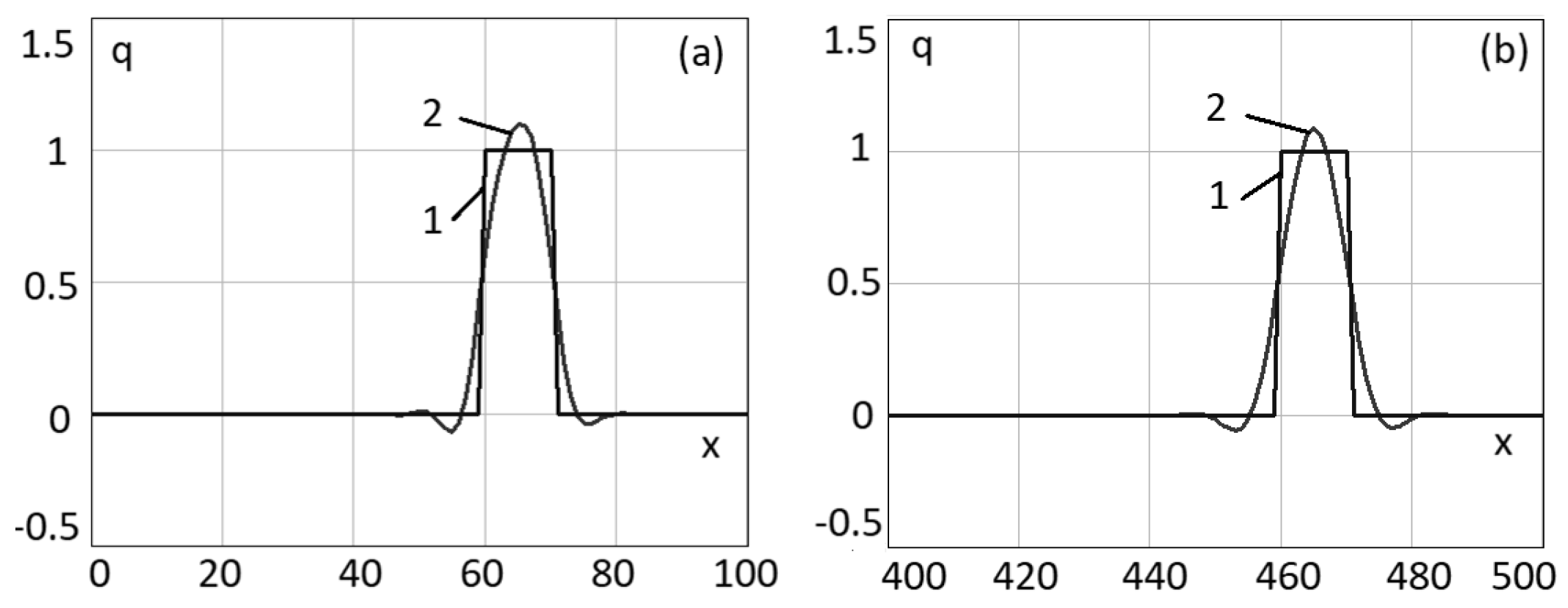
Figure 2 shows the exact solution of test problem I, and a numerical solution based on the scheme (14). The calculated time intervals T were 100 s and 500 s.

4. Stability and Dispersion Properties of the Difference Scheme Obtained as a Linear Combination of the Upwind and Standard Leapfrog Schemes

Let’s use the harmonic method to study the stability of the scheme (14) obtained as a linear combination of the Upwind and Standard Leapfrog schemes. Substitute $q_i^n={\phi }^n{e}^{jki}$ into scheme (14) (case $u\ge 0$):

$$\frac{\phi -1}{\tau }+\frac{4}{3}\left(\frac{e^{-jk}-e^{-jk}/\phi }{2\tau }+u\frac{1-e^{-jk}}{h}\right)+\frac{1-1/\phi }{3\tau }+u\frac{e^{jk}-e^{-jk}}{3h}=0$$

or

$${\phi }^2+\left(\frac{4c-2}{3}\left(1-cosk\right)+\frac{6c-2}{3}jsink\right)\phi -\frac{2cosk+1-2jsink}{3}=0.$$

(15)

The solution of this quadratic equation with respect to $\phi$ is written in the form:

$$\begin{array}{c}\hfill {\phi }_{1,2}=\frac{1-2c}{3}\left(1-cosk\right)+\frac{1-3c}{3}jsink\pm \\ \hfill \pm \sqrt{{\left(\frac{1-2c}{3}\left(1-cosk\right)+\frac{1-3c}{3}jsink\right)}^2+\frac{2cosk+1-2jsink}{3}}.\end{array}$$

(16)

Assume that the calculation takes the value of the root of a complex number with a non-negative real part (the argument of a complex number belongs to a semi-interval $[-\pi /2,\pi /2)$). Let’s consider the case $c=0$:

$${\phi }_{1,2}=\frac{1-e^{-jk}}{3}\pm \sqrt{{\left(\frac{1-e^{-jk}}{3}\right)}^2+\frac{2e^{-jk}+1}{3}}=\frac{1-e^{-jk}}{3}\pm \frac{2+e^{-jk}}{3}.$$

From here, we obtain: ${\phi }_1=1$, ${\phi }_2=\left(-1-2e^{-jk}\right)/3$; therefore, ${\phi }_2$ is not a solution. We studied the values of the function $\left|{\phi }_1(c,k)\right|\in [0,1]$ for $k\in [0,\pi ]$ and $c\in [0,1]$.

Figure 3 shows the values of the module and the argument of the function ${\phi }_1(c,k)$, depending on the values of the parameters k and c.

Let’s study the dispersion properties of scheme (14) in the region of small Courant numbers. Consider the difference between the functions ${\phi }_1(c,k)$ and $\varphi (c,k)=e^{-jck}$:

$$\begin{array}{c}\hfill {\phi }_1(c,k)-\varphi (c,k)=\frac{1-e^{-jk}}{3}-\frac{2c}{3}\left(1-cosk\right)-jcsink+\\ \hfill +\sqrt{{\left(\frac{1-e^{-jk}}{3}-\frac{2c}{3}\left(1-cosk\right)-jcsink\right)}^2+\frac{2e^{-jk}+1}{3}}-e^{-jck}\approx \\ \hfill \approx \frac{1-e^{-jk}}{3}-\frac{2c}{3}\left(1-cosk\right)-jcsink+\\ \hfill +\frac{2+e^{-jk}}{3}\sqrt{1-6\frac{1-e^{-jk}}{{\left(2+e^{-jk}\right)}^2}\left(\frac{2c}{3}\left(1-cosk\right)-jcsink\right)}-e^{-jck}\approx \\ \hfill \approx 1-\frac{2c}{3}\left(1-cosk\right)-jcsink-\frac{1-e^{-jk}}{{\left(2+e^{-jk}\right)}^2}\left(\frac{2c}{3}\left(1-cosk\right)-jcsink\right)-\\ \hfill -cosck+jsinck\approx -c\frac{2\left(1-cosk\right)+\left(1-e^{-jk}\right)jsink}{2+e^{-jk}}=\\ \hfill =\left(-\frac{6+jsink}{2+e^{-jk}}+2+jsink\right)c.\end{array}$$

(17)

Comment 4. From Expression (17), and taking into account the fact that grid refinement leads to a linear increase in the number of layers with respect to time, it follows that for small Courant numbers, the error in solving the transport equation based on scheme (14) is proportional to the function: $f\left(k\right)=\left|-\frac{6+jsink}{2+e^{-jk}}+2+jsink\right|$.

5. Results of Test Calculations

Let’s compare the calculations based on the scheme (14) with the results obtained using other difference schemes.

First, consider a linear combination of the central difference scheme and the Upwind Leapfrog scheme [27]:

$$\begin{array}{c}\hfill \frac{q_i^{n+1}-q_i^n}{\tau }+\frac{q_{i-1}^n-q_{i-1}^{n-1}}{2\tau }+u\frac{q_{i+1}^n+4q_i^n-5q_{i-1}^n}{4h}=0,u\ge 0;\\ \hfill \frac{q_i^{n+1}-q_i^n}{\tau }+\frac{q_{i+1}^n-q_{i+1}^{n-1}}{2\tau }+u\frac{5q_{i+1}^n-4q_i^n-q_{i-1}^n}{4h}=0,u<0.\end{array}$$

(18)

Second, consider a two-parameter difference scheme [28,29]:

$$\frac{q_i^{n+1}-q_i^n}{\tau }+u\frac{{\tilde{q}}_{i+1/2}^n-{\tilde{q}}_{i-1/2}^n}{h}=0,$$

(19)

where ${\tilde{q}}_{i+1/2}^n=\alpha \left(\begin{array}{c}{q}_{i-1}^n\hfill \\ q_{i+2}^n\hfill \end{array}\right)+\left(1-\alpha -\beta \right)\left(\begin{array}{c}{q}_i^n\hfill \\ q_{i+1}^n\hfill \end{array}\right)+\beta \left(\begin{array}{c}{q}_{i+1}^n\hfill \\ q_i^n\hfill \end{array}\right),\begin{array}{c}u\ge 0,\\ u<0.\end{array}$

According to $\alpha =\left(c^2-1\right)/6$ and $\beta =\left(c-1\right)\left(c-2\right)/6$, the accuracy of the scheme (19) is $O\left({\tau }^3+h^3\right)$.

Figure 4 shows the exact solution of the test problem I and numerical solution based on schemes (14), (18), and (19), the Upwind Leapfrog scheme with TVD-limiters, and the Standard Leapfrog scheme with TVD-limiters [27]. The time step is $\tau =0.02$ s (Figure 4a,c and $\tau =0.4$ s, Figure 4b,d). The Courant numbers are 0.01 for Figure 4a,c and 0.2 for Figure 4b,d.

The solution error is calculated using the formula:

$$\mathrm{\Psi }=\sqrt{\frac{{\displaystyle \sum _i}{\left({\tilde{q}}_i-q_i\right)}^2}{{\displaystyle \sum _i}{q}_i^2}},$$

(20)

where $q_i$ is the exact solution value of the problem in the node $i\in {\overline{\omega }}_h$, and ${\tilde{q}}_i$ is the numerical solution that depends on the time step value with a fixed step size in space [30].

Figure 5 shows the values of the errors of the numerical solution (20) of the test problem I depending on the values of the Courant numbers. The length of the time interval is $T=100$ s. Time step $\tau$ takes values from 0.02 s to 2 s. The Courant numbers range from 0.01 to 1.

Figure 6 shows the error function $\mathrm{\Psi }$ of the numerical solution of the test problem I in the norm $L_1$ depending on the length of the calculated time interval.

6. Accuracy of Solving the Heat Conduction Problem

Consider the heat equation with constant coefficients:

$$\frac{\partial q}{\partial t}=\mu \frac{{\partial }^{2}q}{{\partial x}^2}+f,t>0,0<x<L,$$

(21)

$$q\left(x,0\right)=q^0\left(x\right),0\le x\le L,$$

(22)

$$q\left(0,t\right)=q_0\left(t\right),q\left(L,t\right)=q_L\left(t\right),t\ge 0.$$

(23)

We assume the necessary smoothness of the functions included in (21)–(23), and the consistency of the initial and boundary conditions.

Find an analytical solution to the heat conduction problem (21) under certain assumptions. We will assume that the functions in (21) can be represented as finite sums, which are expansions in a finite trigonometric basis:

$$q\simeq \sum _{m=1}^{N-1}{C}_m^{\left(q\right)}\left(t\right)sin\left(\omega mx\right),f\simeq \sum _{m=1}^{N-1}{C}_m^{\left(f\right)}sin\left(\omega mx\right),$$

(24)

where $\omega =\pi /L$, $C_m^{\left(f\right)}=\frac{2}{L}\underset{0}{\overset{L}{\int }}f\left(x\right)sin\left(\omega mx\right)dx$, $C_m^{\left(q\right)}=\frac{2}{L}\underset{0}{\overset{L}{\int }}q\left(x\right)sin\left(\omega mx\right)dx$.

It should be noted that in the case of the tabular method of setting $u_0$, for example, on a spatial grid, the series will be limited to N by the harmonic, and an interpolation trigonometric polynomial is used to restore the continuous function, where N is the number of discrete values of the function.

Next, we consider functions having a derivative of the order $\alpha$ satisfying the inequality $f^{\left(\alpha \right)}\left(x\right)\le K$, with a period of $2\pi$. There is an estimation of the residual term of the series (24) for any natural $\alpha$ [31,32]:

$$sup\left|r\right|=\frac{4K}{{\pi }^2}\frac{lnn}{n^{\alpha }}+O(1/n^{\alpha }),r=u(x/\omega ,t)-\sum _{m=1}^{N-1}C\left(t\right)sin\left(mx\right).$$

Substitute the functions u and f into the heat Equation (21):

$$\frac{\partial \left({\displaystyle \sum _{m=1}^{N-1}}{C}_m^{\left(q\right)}sin\left(\omega mx\right)\right)}{\partial t}=\mu \frac{{\partial }^2\left({\displaystyle \sum _{m=1}^{N-1}}{C}_m^{\left(q\right)}sin\left(\omega mx\right)\right)}{{\partial x}^2}+\sum _{n=1}^{N-1}{C}_m^{\left(f\right)}sin\left(\omega mx\right).$$

(25)

Changing the order of operations of differentiation and summation in (25), and calculating the derivative of a spatial variable:

$$\sum _{m=1}^{N-1}\frac{\partial C_m^{\left(q\right)}\left(t\right)}{\partial t}sin\left(\omega mx\right)=\sum _{m=1}^{N-1}\mu C_m^{\left(q\right)}\left(-{\omega }^2{m}^{2}sin\left(\omega mx\right)\right)+\sum _{n=1}^{N-1}{C}_n^{\left(f\right)}sin\left(\omega mx\right).$$

(26)

Taking into account the linear independence of the functions $sin\left(\omega mx\right)$ for different m, (26) can be written in the form:

$$\frac{\partial C_m^{\left(q\right)}\left(t\right)}{\partial t}=-\mu {\omega }^2{m}^2{C}_m^{\left(q\right)}+C_m^{\left(f\right)}.$$

(27)

The solution of the scheme (27) will take the form:

$$C_m^{\left(q\right)}\left(t\right)=\left(C_m^{\left(q\right)}\left(0\right)-\frac{C_m^{\left(f\right)}}{\mu {\omega }^2{m}^2}\right)e^{-\mu {\omega }^2{m}^{2}t}+\frac{C_m^{\left(f\right)}}{\mu {\omega }^2{m}^2}.$$

(28)

After the transformations, taking into account the given initial and boundary conditions (22) and (23), we obtain the following representation for the solution function [33]:

$$q=\sum _{m=1}^{N-1}\left(\left(C_m^{\left(q\right)}\left(0\right)-\frac{C_m^{\left(f\right)}}{\mu {\omega }^2{m}^2}\right)e^{-\mu {\omega }^2{m}^{2}t}+\frac{C_m^{\left(f\right)}}{\mu {\omega }^2{m}^2}\right)sin\left(\omega mx\right).$$

(29)

Difference scheme for the heat equation. For the numerical solution of the problem (21), we use the uniform computational grid (2). Then, the discrete analog of (21) can be written in the form:

$$\frac{q_i^{n+1}-q_i^n}{\tau }=\mu \frac{q_{i+1}^{n+\sigma }-2q_i^{n+\sigma }+q_{i-1}^{n+\sigma }}{h^2}+f_i^{n+\sigma },$$

(30)

where $q_i^{n+\sigma }=\sigma q_i^{n+1}+\left(1-\sigma \right)q_i^n$, $\sigma \in \left[0,1\right]$—weight of the scheme [34].

The necessary stability condition (case $\sigma =0$) obtained on the basis of the harmonic method leads to the following inequality [2,3]:

$$\gamma =\frac{\tau \mu }{h^2}\le \frac{1}{2}.$$

(31)

Despite the fact that estimate (31) is a strict limitation for explicit difference schemes, in practice, the time step should be taken even less.

Test problem II. Find the solution of the equation:

$$\frac{\partial q}{\partial t}=\mu \frac{{\partial }^{2}q}{{\partial x}^2},\mu =1m^2/s,0\le t\le T,0\le x\le L,q\left(t,0\right)=0$$

with initial conditions: $q^0\left(x\right)=\theta (20-x)-\theta (10-x)$.

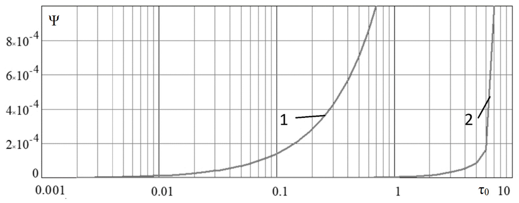
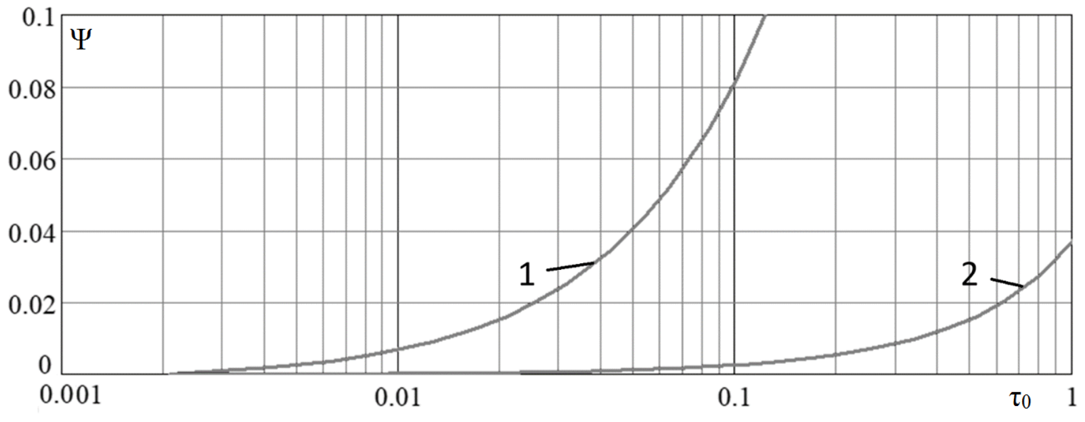
Parameters of the calculation grid: the time step $\tau$ is in the range from 0.001 s to 10 s, the space step $h=1$ m, and the length of the time interval $T=60$ s.

Figure 7 shows the error of solving test problem II based on the scheme (30). The calculation error is calculated using the Formula (20). The value of the time step ${\tau }_0$ related to the value ${\tau }_{max}=h^2/2\mu$ (obtained from Equation (31)) is postponed along the horizontal axis $\left({\tau }_0=\tau /{\tau }_{max}\right)$.

In order for the percentage error of the explicit scheme (30) to be equal to 0.01 %, it is necessary to take the value ${\tau }_0=0.0717$; in the case of using the proposed scheme with weights, the parameter is ${\tau }_0=5.1858$.

Test problem III. Consider the problem that arises when modeling the transport of suspended matter in shallow reservoirs. Find a solution to the two-dimensional diffusion equation for a region elongated in one direction:

$$\frac{\partial q}{\partial t}={\mu }_x\frac{{\partial }^{2}q}{{\partial x}^2}+{\mu }_y\frac{{\partial }^{2}q}{{\partial y}^2},t>0,0<x<L_{x}0<y<L_y,$$

with initial conditions $q\left(x,y,t\right)\left|{}_{t=0}\right.=\left(\theta (1100-x)-\theta (900-x)\right)\left(\theta (3-y)-\theta (2-y)\right)$, where $0\le x\le L_x$, $0\le y\le L_y$ and boundary conditions are in Dirichlet form.

For the numerical solution of the test problem III, we introduce a uniform computational grid $\omega ={\overline{\omega }}_h\times {\omega }_{\tau }$, where ${\overline{\omega }}_h=\left\{x_i=i{h}_x,y_j=j{h}_y,i=\overline{0,N_x},j=\overline{0,N_y},\right.$

$\left.N_x{h}_x=L_x,N_y{h}_y=L_y\right\}$, where $h_x=x_{i+1}-x_i=const$ and $h_y=y_{j+1}-y_j=const$ are the space steps; $N_x$ and $N_y$ are the number of nodes in space; $L_x$ and $L_y$ are the characteristic dimension of the computational domain, ${\omega }_{\tau }=\left\{\left.t^n\right|t^n=n\tau ,n=\overline{0,N_t},N_t\tau =T\right\}$, where $\tau =t^{n+1}-t^n=const$ is the time step; $N_t$ is the number of time layers; and T is the upper bound in time.

The discrete analog of test problem III can be written in the form:

$$\frac{q_{i,j}^{n+1}-q_{i,j}^n}{\tau }={\mu }_x\frac{q_{i+1,j}^{n+\sigma }-2q_{i,j}^{n+\sigma }+q_{i-1,j}^{n+\sigma }}{h_x^2}+{\mu }_y\frac{q_{i,j+1}^{n+\sigma }-2q_{i,j}^{n+\sigma }+q_{i,j-1}^{n+\sigma }}{h_y^2},$$

(32)

where $q_{i,j}^{n+\sigma }=\sigma q_{i,j}^{n+1}+\left(1-\sigma \right)q_{i,j}^n$, $\sigma \in \left[0,1\right]$—weight of the scheme [34].

Parameters of test problem III: ${\mu }_x$ = 100 m²/s, ${\mu }_y=0.5{\mathrm{m}}^2/\mathrm{s}$, $L_x=2000$ m, $L_y=5$ m.

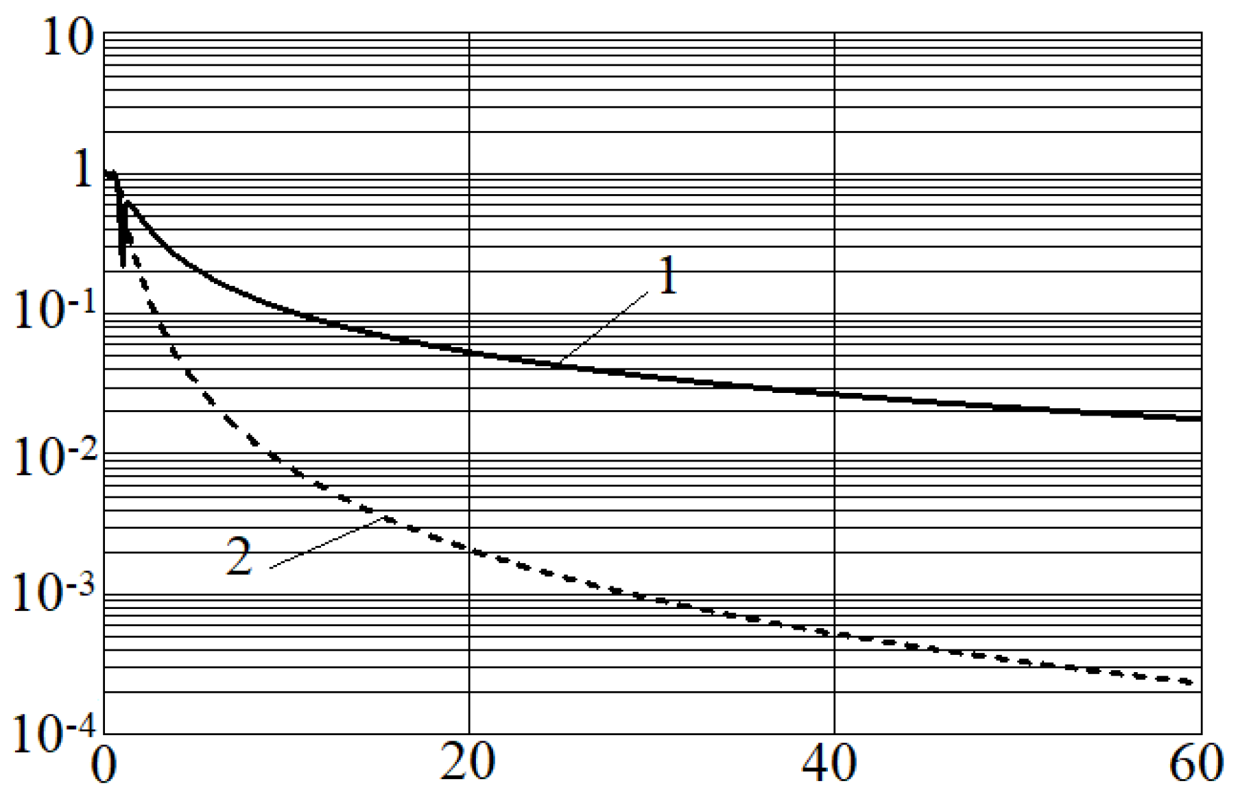
Parameters of the calculation grid: steps in the space are $h_x=100$ m and $h_y=0.5$ m; the time step $\tau$ is in the range from 0.001 s to 10 s, and the length of the time interval is $T=600$ s. Figure 8 shows solutions to test problem III based on scheme (30).

From Figure 7 and Figure 8, we see that in order to achieve the same approximation error, the time step limit for an explicit scheme is significantly stricter than for a scheme with weights. In order for the percentage error of the explicit scheme to be equal to 1 %, it is necessary to take the value ${\tau }_0=0.01376$; in the case of using the scheme (30) with weights, the parameter is ${\tau }_0=0.34844$.

Comment 5. The solution obtained on the basis of scheme (30) in the case of $\sigma =0$, i.e., based on the explicit scheme, is stable under the constraint $\tau \le O\left(h^2\right)$ [35]. Scheme (30) at $\sigma \ge 0.5$ has no time step restrictions. In practice, when solving problems based on the difference scheme (30) in the case of $\sigma \in [0,1]$, it is recommended to use the constraint $\tau \le \Delta \times {\left({\sum }_{i=1}^r\left(2{\mu }_i/h_i\right)\right)}^{-1}$, where r is the dimension of space and the parameter $\Delta \sim \tau /{\tau }_{max}$, where $\tau$ is the size of the time step that must be taken so that the calculation error is in an acceptable range, and ${\tau }_{max}$ is the size of the time step obtained from stability conditions for the explicit scheme, while the constraint ${\tau }_0\le \Delta$ is satisfied. In the general case, for solving problems of diffusion–convection, the value of the parameter $\Delta$ is determined on the basis of computational expediency: if the step $\tau$ is taken too large, then the calculation error will be large, and if the step $\tau$ is small, then the computational costs will be high. For scheme (30), at $\sigma =0$, it is recommended to use the value $\Delta =0.01$, and at $\sigma =0.5$, it is recommended to use the value $\Delta =0.3$.

Comment 6.Figure 5b shows that in the case of values of the Courant number up to 0.1, the proposed scheme (14) for solving test problem I (convection problem) is more accurate than the Upwind Leapfrog difference scheme with TVD-limiters. From the solutions of the test problem II and the test problem III (diffusion problem) based on scheme (30) at $\sigma =0$ and with respect to Comment 5, a constraint on the time step $\tau \le \Delta \times {\tau }_{max}$ was obtained, where $\Delta =0.01$, ${\tau }_{max}=h^2⁄2\mu$. Based on the obtained constraints on the value of the Courant number $c=\left|u\right|\tau /h\le 0.1$ with the limitation on the time step, we obtain $\Delta \left|u\right|h/2\mu \le 0.1$ or $Pe\le \left(2\times 0.1\right)/\Delta =20$, where $Pe=\left|u\right|h/\mu$ is the grid Péclet number [36]. Note that we consider the case of the absence of monotonicity of schemes constructed on the basis of central-difference approximations (the case $Pe>2$). Therefore, the proposed approximation of the convective transport operator is effective for $2\le Pe\le 20$.

7. Accuracy of Modified Difference Scheme

Consider the nonstationary convection–diffusion equation [37]:

$$\frac{\partial q}{\partial t}+u\frac{\partial q}{\partial x}=\mu \frac{{\partial }^{2}q}{\partial x^2},0<t<T,0<x<L,u=const$$

(33)

with initial and boundary conditions: $q\left(0,x\right)=q^0\left(x\right)$, $q\left(t,0\right)=q\left(t,L\right)=0$.

For exact solution of Equation (33), write the finite sum of the trigonometric Fourier series for the function $q(x,t)$ in complex form:

$$q(x,t)=\sum _{m=-N}^N{C}_m\left(t\right)exp\left(j\omega mx\right),$$

(34)

where $j=\sqrt{-1}$, $\omega =\pi /L$, m is number of modes, and $C_m\left(t\right)=\frac{2}{L}\underset{0}{\overset{L}{\int }}q(x,t)exp\left(j\omega mx\right)dx$ is complex amplitude of the m-th mode.

Substitute (34) in (33):

$$\begin{array}{c}\hfill \frac{\partial }{\partial t}\left(\sum _{m=-N}^N{C}_m\left(t\right)exp\left(j\omega mx\right)\right)+u\frac{\partial }{\partial x}\left(\sum _{m=-N}^N{C}_m\left(t\right)exp\left(j\omega mx\right)\right)=\\ \hfill =\mu \frac{{\partial }^2}{\partial x^2}\left(\sum _{m=-N}^N{C}_m\left(t\right)exp\left(j\omega mx\right)\right)\end{array}$$

or

$$\begin{array}{c}\hfill \sum _{m=-N}^N\frac{\partial C_m\left(t\right)}{\partial t}exp\left(j\omega mx\right)+u\sum _{m=-N}^{N}j\omega m{C}_m\left(t\right)exp\left(j\omega mx\right)=\\ \hfill =\mu \sum _{m=-N}^N{\omega }^2{m}^2{C}_m\left(t\right)exp\left(j\omega mx\right).\end{array}$$

The functions $exp\left(jm\omega x\right)$ are linearly independent; therefore, the last equation can be written in the form:

$$\frac{\partial C_m\left(t\right)}{\partial t}=-\left(ju\omega m+\mu {\omega }^2{m}^2\right)C_m\left(t\right).$$

(35)

The solution of Equation (35) has the form:

$$C_m\left(t\right)=C_m\left(0\right)exp\left(-\left(ju\omega m+\mu {\omega }^2{m}^2\right)t\right).$$

(36)

Based on the initial and boundary conditions for (33), (34), and (36), the exact solution of Equation (33) can be written in the form:

$$q(x,t)=\sum _{m=-N}^N{C}_m\left(0\right)exp\left(-\left(ju\omega m+\mu {\omega }^2{m}^2\right)t\right)exp\left(j\omega mx\right),$$

(37)

Consider the case $u\ge 0$. For a numerical solution of the problem (33), we use the uniform grid (2). The approximation of Equation (33) has the form:

$$\begin{array}{c}\hfill \frac{q_i^{n+1}-q_i^n}{\tau }+\frac{4}{3}\left(\frac{q_{i-1}^n-q_{i-1}^{n-1}}{2\tau }+u\frac{q_i^n-q_{i-1}^n}{h}\right)+\frac{q_i^n-q_i^{n-1}}{3\tau }+\\ \hfill +u\frac{q_{i+1}^n-q_{i-1}^n}{3h}=2\mu \frac{q_{i+1}^n-2q_i^n+q_{i-1}^n}{h^2},\end{array}$$

or

$$\begin{array}{c}\hfill \frac{q_i^{n+1}-q_i^n}{\tau }+2\frac{q_{i-1}^n-q_{i-1}^{n-1}}{3\tau }+\frac{q_i^n-q_i^{n-1}}{3\tau }+u\frac{q_{i+1}^n+4q_i^n-5q_{i-1}^n}{3h}=\\ \hfill =2\mu \frac{q_{i+1}^n-2q_i^n+q_{i-1}^n}{h^2},\end{array}$$

(38)

where

$$q_i=\sum _{m=-N}^N{C}_{m}exp\left(j\omega m{x}_i\right).$$

(39)

Substitute (39) in (38):

$$\begin{array}{c}\hfill \sum _{m=-N}^N\frac{C_m^{n+1}-C_m^n}{\tau }exp\left(j\omega mhi\right)+\\ \hfill +2\sum _{m=-N}^N\frac{C_m^n-C_m^{n-1}}{3\tau }exp\left(j\omega mh(i-1)\right)+\sum _{m=-N}^N\frac{C_m^n-C_m^{n-1}}{3\tau }exp\left(j\omega mhi\right)+\\ \hfill +u\sum _{m=-N}^N\frac{C_m^{n}exp\left(j\omega mh\right)+4C_m^n-5C_m^{n}exp\left(-j\omega mh\right)}{3h}exp\left(j\omega mhi\right)-\\ \hfill -2\mu \sum _{m=-N}^N\frac{C_m^{n}exp\left(j\omega mh\right)-2C_m^n+C_m^{n}exp\left(-j\omega mh\right)}{h^2}exp\left(j\omega mhi\right)=0,\end{array}$$

(40)

The functions $exp\left(jm\omega hi\right)$ are linearly independent; therefore, (40) can be written in the form:

$$\begin{array}{c}\hfill \frac{C_m^{n+1}-C_m^n}{\tau }+2\frac{C_m^n-C_m^{n-1}}{3\tau }exp\left(-j\omega mh\right)+\frac{C_m^n-C_m^{n-1}}{3\tau }+\\ \hfill +u{C}_m^n\frac{exp\left(j\omega mh\right)+4-5exp\left(-j\omega mh\right)}{3h}-\\ \hfill -2\mu C_m^n\frac{exp\left(j\omega mh\right)-2+exp\left(-j\omega mh\right)}{h^2}=0.\end{array}$$

(41)

When $\tau \to 0$, (41) takes the form:

$$\begin{array}{c}\hfill \frac{\partial C_m\left(t\right)}{\partial t}\left(\frac{4}{3}+\frac{2}{3}exp\left(-j\omega mh\right)\right)+u{C}_m^n\frac{exp\left(j\omega mh\right)+4-5exp\left(-j\omega mh\right)}{3h}-\\ \hfill -2\mu C_m^n\frac{exp\left(j\omega mh\right)-2+exp\left(-j\omega mh\right)}{h^2}=0\end{array}$$

or

$$\begin{array}{c}\hfill \frac{\partial C_m\left(t\right)}{\partial t}=\left(-u\frac{exp\left(j\omega mh\right)+4-5exp\left(-j\omega mh\right)}{2h\left(2+exp\left(-j\omega mh\right)\right)}+\right.\\ \hfill +\left.3\mu \frac{exp\left(j\omega mh\right)-2+exp\left(-j\omega mh\right)}{h^2\left(2+exp\left(-j\omega mh\right)\right)}\right)C_m^n.\end{array}$$

(42)

Lemma 1.

When approximating problem (33) using the difference scheme (38) for each mode of solution function q, the convective exchange rate u and the diffusion exchange rate μ are less than the real values, and differ by

$${\alpha }_1=1-\frac{exp\left(j\omega mh\right)+4-5exp\left(-j\omega mh\right)}{2j\omega mh\left(2+exp\left(-j\omega mh\right)\right)}$$

and

$${\alpha }_2=1-\frac{3\left(-exp\left(j\omega mh\right)+2-exp\left(-j\omega mh\right)\right)}{{\omega }^2{m}^2{h}^2\left(2+exp\left(-j\omega mh\right)\right)},$$

respectively.

Proof. 

Scheme (42) can be written in the form:

$$\begin{array}{c}\hfill \frac{\partial C_m\left(t\right)}{\partial t}=\left(-uj\omega m\frac{exp\left(j\omega mh\right)+4-5exp\left(-j\omega mh\right)}{2j\omega mh\left(2+exp\left(-j\omega mh\right)\right)}+\right.\\ \hfill +\left.3\mu {\omega }^2{m}^2\frac{exp\left(j\omega mh\right)-2+exp\left(-j\omega mh\right)}{{\omega }^2{m}^2{h}^2\left(2+exp\left(-j\omega mh\right)\right)}\right)C_m^n.\end{array}$$

Taking into account (36), the last expression, which is a solution based on the difference scheme (38), corresponds to the solution of the equation

$$\frac{\partial q}{\partial t}+u^{*}\frac{\partial q}{\partial x}={\mu }^{*}\frac{{\partial }^{2}q}{\partial x^2},$$

where $u^{*}=u\left(1-{\alpha }_1\right)$, ${\mu }^{*}=\mu \left(1-{\alpha }_2\right)$, where

$${\alpha }_1=1-\frac{exp\left(j\omega mh\right)+4-5exp\left(-j\omega mh\right)}{2j\omega mh\left(2+exp\left(-j\omega mh\right)\right)},$$

$${\alpha }_2=1-\frac{3\left(-exp\left(j\omega mh\right)+2-exp\left(-j\omega mh\right)\right)}{{\omega }^2{m}^2{h}^2\left(2+exp\left(-j\omega mh\right)\right)}.$$

□

Analyze the approximation error of the convective term in space. Let’s introduce replacement $j\omega mh=s$, when

$${\alpha }_1=1-\frac{e^s+4-5e^{-s}}{2s\left(2+e^{-s}\right)}.$$

(43)

Let’s use the decomposition of the functions $e^{\pm s}$ in the Maclaurin series:

$$e^{\pm s}=1\pm s+\frac{s^2}{2}\pm \frac{s^3}{6}+\frac{s^4}{24}\pm \frac{s^5}{120}+O\left(s^6\right).$$

(44)

Substitute (44) in (43):

$$\begin{array}{c}\hfill {\alpha }_1=1-\frac{1+s+s^2/2+s^3/6+s^4/24+s^5/120+4+O\left(s^6\right)}{2s\left(2+1-s+s^2/2-s^3/6+s^4/24-s^5/120+O\left(s^6\right)\right)}-\\ \hfill -\frac{5-5s+5s^2/2-5s^3/6+5s^4/24-s^5/24+O\left(s^6\right)}{2s\left(2+1-s+s^2/2-s^3/6+s^4/24-s^5/120+O\left(s^6\right)\right)}=\\ \hfill =1-\frac{6s-2s^2+s^3-s^4/6+s^5/20+O\left(s^6\right)}{6s-2s^2+s^3-s^4/3+s^5/12+O\left(s^6\right)}-\\ \hfill =\frac{-s^4/6+s^5/30+O\left(s^6\right)}{6s-2s^2+s^3-s^4/3+s^5/12+O\left(s^6\right)}=-\frac{s^3}{36}+O\left(s^4\right),\end{array}$$

or

$${\alpha }_1=j\frac{{\left(\omega mh\right)}^3}{36}+O\left({\left(\omega mh\right)}^4\right).$$

(45)

From the Expression (45), we can obtain that scheme (34) approximates the convective term of Equation (33) with the third order of accuracy in space.

Analyze the approximation error of the diffusion term in space:

$$\begin{array}{c}\hfill {\alpha }_2=1+\frac{3\left(-e^s+2-e^{-s}\right)}{s^2\left(2+e^{-s}\right)}=1+\frac{-3-3s-3s^2/2-s^3/2-s^4/8+O\left(s^5\right)}{s^2\left(2+1-s+s^2/2-s^3/6+s^4/24+O\left(s^5\right)\right)}+\\ \hfill +\frac{6-3+3s-3s^2/2+s^3/2-s^4/8+O\left(s^5\right)}{s^2\left(2+1-s+s^2/2-s^3/6+s^4/24+O\left(s^5\right)\right)}=1+\frac{-3s^2-s^4/4+O\left(s^5\right)}{3s^2-s^3+s^4/2+O\left(s^5\right)}=\\ \hfill =\frac{-s^3-s^4/4+O\left(s^5\right)}{3s^2-s^3+s^4/2+O\left(s^5\right)}=-\frac{s}{3}+O\left(s^2\right),\end{array}$$

or

$${\alpha }_2=-\frac{j\omega mh}{3}+O\left({\left(\omega mh\right)}^2\right).$$

(46)

From the Expression (46), we can obtain that the scheme (38) approximates the diffusion term of Equation (33) with the first order of accuracy in space.

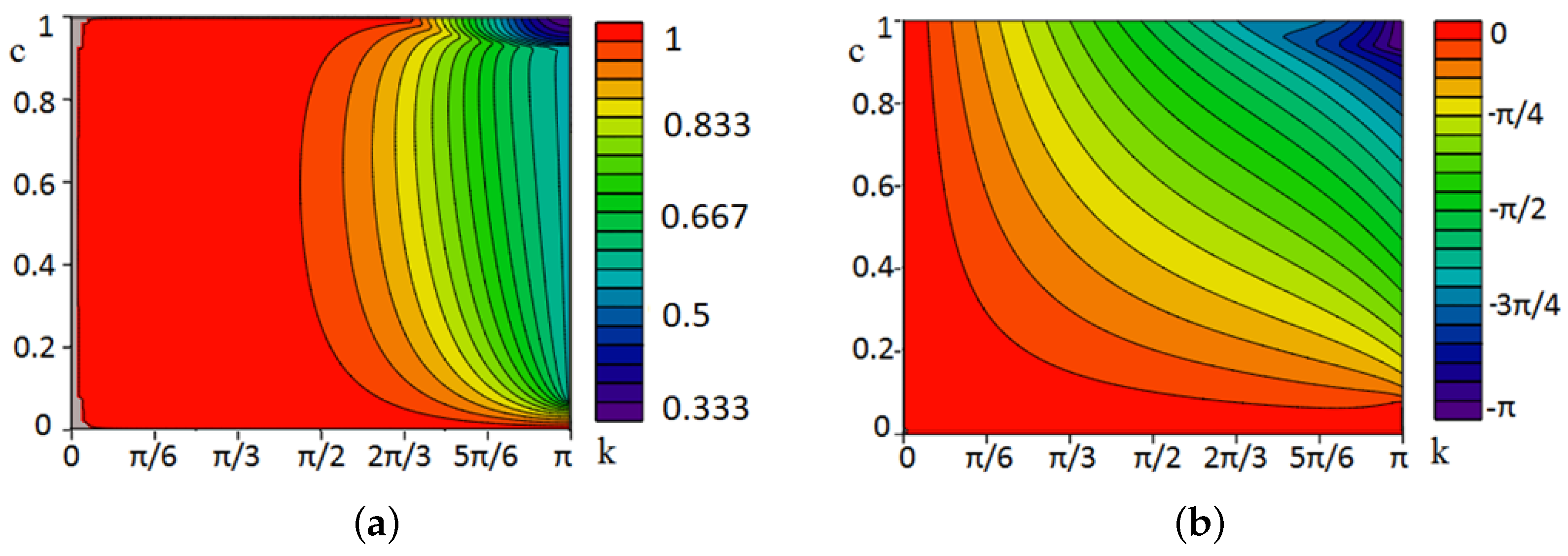
Note that the variable $r=\pi /\omega mh$ describes the number of nodes per half wave period, and $\pi >\omega mh$. Therefore, the accuracy of the solution depends on the number of nodes per half wave period.

Figure 9 and Figure 10 show functions

$${\alpha }_1\left(r\right)=1-\frac{exp\left(j\pi /r\right)+4-5exp\left(-j\pi /r\right)}{2j\pi /r\left(2+exp\left(-j\pi /r\right)\right)}$$

and

$${\alpha }_2\left(r\right)=1-\frac{3\left(-exp\left(j\pi /r\right)+2-exp\left(-j\pi /r\right)\right)}{{\pi }^2/r^2\left(2+exp\left(-j\pi /r\right)\right)},$$

that describe the dependence of the approximation error of the convective and diffusion terms, respectively, by the difference scheme (38) on the number of nodes in comparison with the central difference scheme [1].

Based on Figure 9 and Figure 10, we can conclude that difference scheme (38) is applicable for problems in which convective transport prevails over diffusion.

8. Approximation of the Convection–Diffusion Problem

To approximate the convection operator in problem (33), we will use the difference operator of the scheme obtained as a result of a linear combination of the Upwind and Standard Leapfrog schemes:

$$\begin{array}{c}\hfill \frac{q_i^{n+1}-q_i^n}{\tau }+2\frac{q_{i-1}^n-q_{i-1}^{n-1}}{3\tau }+\frac{q_i^n-q_i^{n-1}}{3\tau }+u\frac{q_{i+1}^n+4q_i^n-5q_{i-1}^n}{3h}=\\ \hfill =2\mu \frac{q_{i+1}^n-2q_i^n+q_{i-1}^n}{h^2},u\ge 0;\\ \hfill \frac{q_i^{n+1}-q_i^n}{\tau }+2\frac{q_{i+1}^n-q_{i+1}^{n-1}}{3\tau }+\frac{q_i^n-q_i^{n-1}}{3\tau }+u\frac{5q_{i+1}^n-4q_i^n-q_{i-1}^n}{3h}=\\ \hfill =2\mu \frac{q_{i+1}^n-2q_i^n+q_{i-1}^n}{h^2},u<0.\end{array}$$

(47)

Test problem IV. Find a solution to the equation:

$$\frac{\partial q}{\partial t}+u\frac{\partial q}{\partial x}=\mu \frac{{\partial }^{2}q}{\partial x^2},u=0.5\mathrm{m}/\mathrm{s},\mu =const,0<t<T,0<x<L$$

with initial condition $q\left(0,x\right)=q^0\left(x\right)=\theta (20-x)-\theta (10-x)$ and boundary conditions $q\left(t,0\right)=q\left(t,L\right)=0$.

The exact solution of the test problem IV can be represented as [33]:

$$q\left(t,x\right)=\sum _{m=1}^{N-1}{c}_m^0{e}^{-\mu {\omega }^2{m}^{2}t}sin\left(\omega mx\right),c_m^0=\frac{2}{L}{\int }_0^L{q}^0(x+ut)sin\left(\omega mx\right)dx,\omega =\frac{\pi }{L}.$$

In Figure 11, the exact solution of the test problem IV and the numerical solutions based on the scheme (47), and the Upwind Leapfrog difference scheme with TVD-limiters are presented. The test problem IV is considered for different values of the diffusion operator $\mu$ = 0.025 m²/s (in this case, $Pe=20$) and $\mu$ = 0.0025 m²/s ($Pe=200$).

Parameters of the calculation grid: the step in space $h=1$ m, the time step $\tau =0.02s$, the length of the spatial interval $L=200$ m, and the length of the time interval T = 100 s.

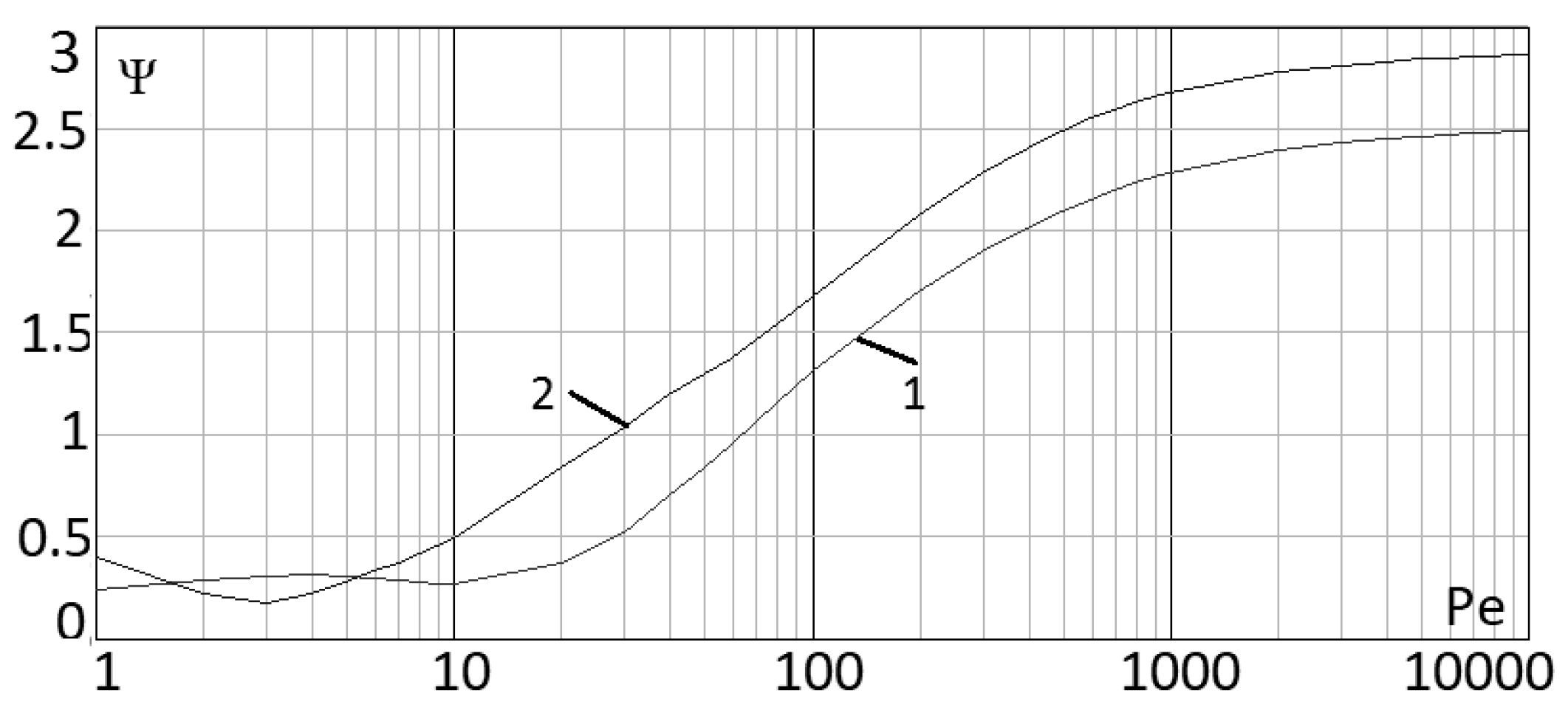
Figure 12 shows the error function $\mathrm{\Psi }$ (in the norm $L_1$) of the numerical solution of the test problem IV based on the difference scheme (47) and the Upwind Leapfrog difference scheme with TVD-limiters, depending on the values of the grid Péclet number.

Figure 12 illustrates that the difference scheme (47) for solving the problem (33) has an insignificant error in a wide range of values of grid Péclet numbers.

The approximation of the problem (33) based on explicit central difference schemes can be written in form:

$$\frac{q_i^{n+1}-q_i^n}{\tau }+u\frac{q_{i+1}^n-q_{i-1}^n}{2h}=\mu \frac{q_{i+1}^n-2q_i^n+q_{i-1}^n}{h^2}.$$

(48)

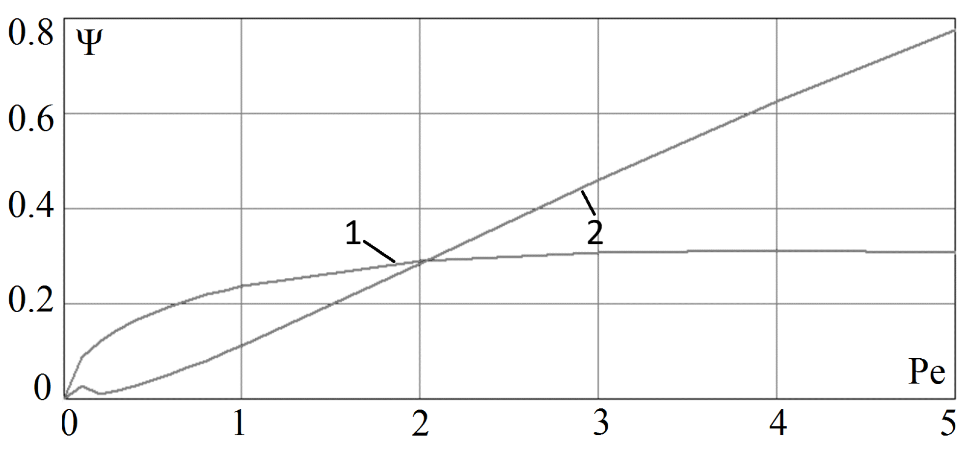
Figure 13 shows the error function $\mathrm{\Psi }$ (in the norm $L_1$) of the numerical solution of the test problem IV (47) and the central difference scheme (48), depending on values of the grid Péclet number.

Figure 13 shows the error function $\mathrm{\Psi }$ (in the norm $L_1$) that occurs when approximating the solution of test problem IV. The difference scheme (47) and the central difference scheme (48) were used in this case. The value of the approximation error is plotted along the Oy axis, and the value of the grid Péclet number is plotted along the Ox axis. The space step $h=1$ m, the time step $\tau =0.02$, the value of the spatial interval $L=200$ m, the value of the time interval T is 100 s, and the range for the diffusion coefficient—from $5\times {10}^{-3}$ to 5 m²/s, for these graphs.

Comment 7.Figure 13, which demonstrates the calculation error of the test problem IV, shows that the central difference scheme (48) has a higher accuracy compared to the difference scheme (47) for $0\le Pe\le 2$. Thus, the proposed modification of the Upwind Leapfrog schemes (47) in this paper has a smaller error compared to other considered difference schemes for solving the problems of continuous medium transport described by the diffusion–convection equation in the range of grid Péclet numbers from 2 to 20.

9. Discussion

The proposed difference scheme is a linear combination of the Upwind Leapfrog scheme with a 2/3 weight coefficient, and the Standard Leapfrog scheme with a 1/3 weight coefficient. The weight coefficients were determined as a result of solving the problem of minimizing the approximation error. This scheme practically does not have grid viscosity when solving convection–diffusion problems; therefore, it allows for more accurate solutions to be obtained in the case of a significant predominance of convective processes over diffusion ones. When modeling hydrodynamic processes in real areas with complex geometry (currents in river channels, estuary zones, along areas of land strongly protruding into the sea—sand bars), large values of grid Péclet numbers arise. The application of the developed vortex-resolving scheme to the problems of hydrodynamics allows small-sized vortexes that occur in coastal systems to be more accurately reproduced.

The proposed difference scheme has an advantage over the classical Upwind and Standard Leapfrog schemes in the case of small Courant numbers. In [24], the approximation error of the developed scheme, which is equal to $O\left(c{h}^2\right)$, is researched, while for classical schemes, the approximation errors are equal to $O\left(h^2\right)$. However, for cases of interest from the point of view of applications, the constant c is much less than unity, which implies the advantage of the proposed difference scheme.

In the process of the numerical experiments, we compared the approximation error in the norm of the grid space $L_1$ for the proposed difference scheme, the scheme that is a linear combination of the Upwind Leapfrog scheme, and the scheme with central differences, as well as the two-parameter difference scheme, which has the third order of accuracy for solving the convection–diffusion problem. The constructed graphs showed the dependence of the errors in solving test problems on the values of the Courant numbers. The study showed that the proposed difference scheme and the scheme based on a linear combination of the Upwind Leapfrog scheme and the central difference scheme have a smaller error compared to other considered schemes. In addition, the developed difference scheme, based on a linear combination of the Upwind and Standard Leapfrog schemes, has an advantage in approximation accuracy compared to other considered schemes for the case of Péclet number values from 2 to 20.