
Analysis of Electromagnetic Scattering from Large Arrays of Cylinders via a Hybrid of the Method of Auxiliary Sources (MAS) with the Fast Multipole Method (FMM)

 ,
,  and
and 
Abstract
:1. Introduction
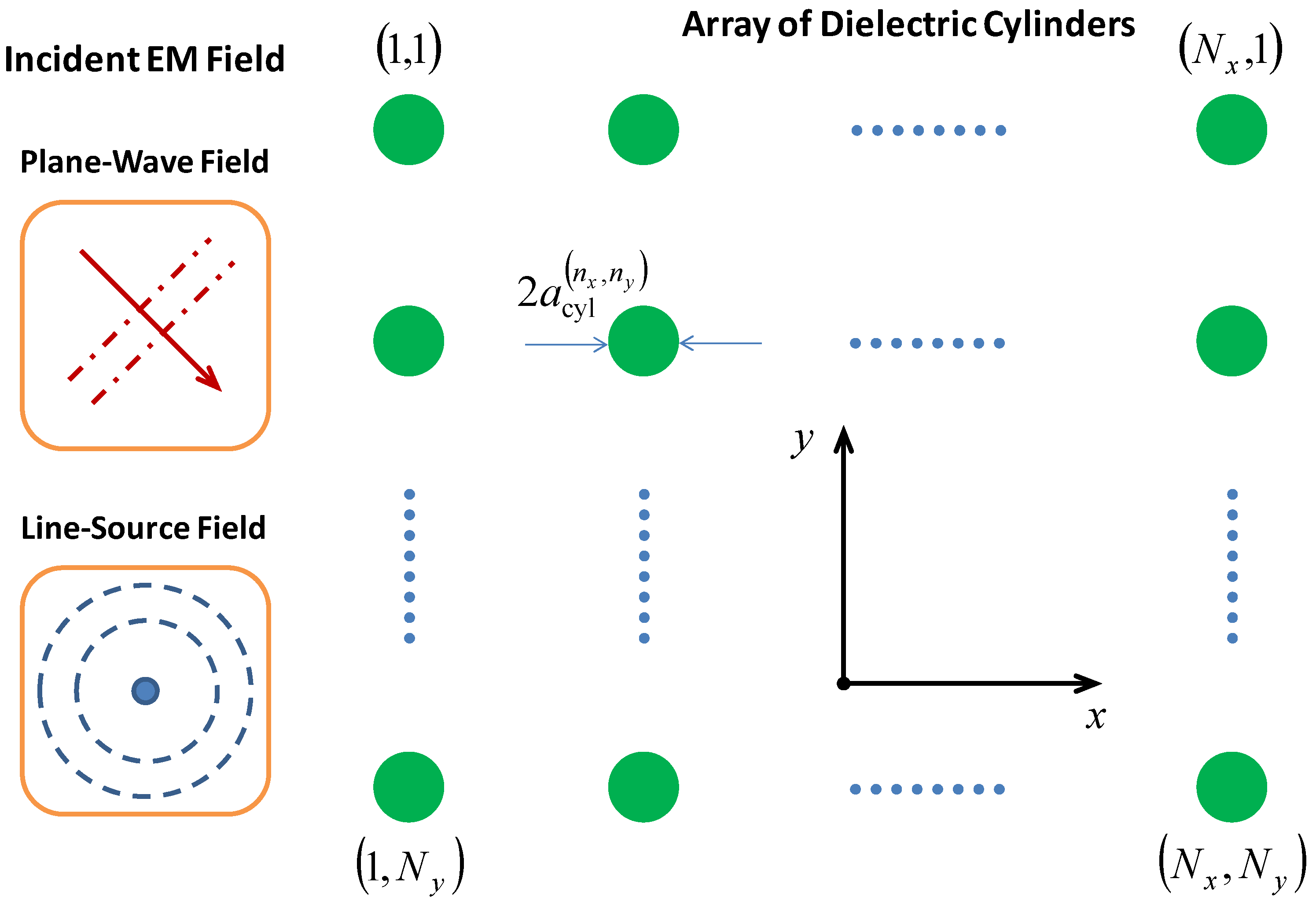
2. Problem Description
3. Formulation
3.1. Standard MAS Formulation
3.2. Hybrid MAS-FMM Formulation
4. Numerical Results and Discussion
5. Conclusions and Prospect
- The treatment of random lattices of cylinders for the deterministic or stochastic analysis of electromagnetic propagation through complex vegetation environments (like forests) is quite simple and straightforward. It is particularly stressed that macroscopic, stochastic approaches may be best suited for characterizing complex vegetation environments. For this purpose, one can start from the assumption of proper statistical distributions for the radii of the cylinders and the distances between them (depending on the specific characteristics of the orchard/forest or other environment of interest), proceed using some certain strategy for applying the MAS-FMM scheme of this work repeatedly, and finally compute distributions or moments for the statistical characterization of the propagation environment of interest.
- The generalization of the proposed MAS-FMM scheme to cope with 3D scatterers. Though not easy to manipulate and present in a comprehensive manner, this can be accomplished via lengthy but straightforward modifications [1].
- The systematic assessment of the proposed MAS-FMM scheme from the aspect of the associated complexity and computational cost and the relevant comparisons with other established methods of Computational Electromagnetics. To this end, rigorous cost metrics, such as polynomials involving the total number of unknowns, could be obtained, and subsequently utilized to provide a solid basis for cost comparisons. Furthermore, apart from the cost metrics usually used pertaining to the execution time and memory usage, one possible measure of the computational cost could be the number of machine cycles consumed by the deployed routines (i.e., matrix filling, system solving, calculation of currents and/or fields, etc.). Such an analysis is beyond the scope of the present paper and is left for a future investigation.
Author Contributions
Funding
Institutional Review Board Statement
Informed Consent Statement
Data Availability Statement
Acknowledgments
Conflicts of Interest
References
- Kaklamani, D.I.; Anastassiu, H.T. Aspects of the Method of Auxiliary Sources (MAS) in Computational Electromagnetics. IEEE Antennas Propag. Mag. 2002, 44, 48–64. [Google Scholar] [CrossRef]
- Wriedt, T.; Eremin, Y.A. (Eds.) The Generalized Multipole Technique for Light Scattering—Recent Developments; Springer: Cham, Switzerland, 2018. [Google Scholar]
- Avdikos, G.K.; Anastassiu, H.T. Computational Cost Estimations and Comparisons for Three Methods of Applied Electromagnetics (MoM, MAS, MMAS). IEEE Antennas Propag. Mag. 2005, 47, 121–129. [Google Scholar] [CrossRef]
- Fikioris, G.; Tsitsas, N.L. Convergent Fields Generated by Divergent Currents in the Method of Auxiliary Sources. In The Generalized Multipole Technique for Light Scattering—Recent Developments; Wriedt, T., Eremin, Y.A., Eds.; Springer Series on Atomic, Optical, and Plasma Physics: Berlin/Heidelberg, Germany, 2018; Volume 99, pp. 93–119. [Google Scholar]
- Leviatan, Y. Analytic Continuation Considerations when Using Generalized Formulations for Scattering Problems. IEEE Trans. Antennas Propag. 1990, 38, 1259–1263. [Google Scholar] [CrossRef]
- Anastassiu, H.T.; Kaklamani, D.I. Error Estimation and Optimization of the Method of Auxiliary Sources (MAS) for Scattering from a Dielectric Cylinder. Radio Sci. 2004, 39, RS5015. [Google Scholar] [CrossRef]
- Fikioris, G. On Two Types of Convergence in the Method of Auxiliary Sources. IEEE Trans. Antennas Propag. 2006, 54, 2022–2033. [Google Scholar] [CrossRef]
- Tsitsas, N.L.; Alivizatos, E.G.; Anastassiu, H.T.; Kaklamani, D.I. Optimization of the Method of Auxiliary Sources (MAS) for Oblique Incidence Scattering by an Infinite Dielectric Cylinder. Electr. Eng. 2007, 89, 353–361. [Google Scholar] [CrossRef]
- Valagiannopoulos, C.A.; Tsitsas, N.L.; Fikioris, G. Convergence Analysis and Oscillations in the Method of Fictitious Sources Applied to Dielectric Scattering Problems. J. Opt. Soc. Am. A 2012, 29, 1–10. [Google Scholar] [CrossRef]
- Tsitsas, N.L.; Zouros, G.P.; Fikioris, G.; Leviatan, Y. On Methods Employing Auxiliary Sources for 2-D Electromagnetic Scattering by Non-Circular Shapes. IEEE Trans. Antennas Propag. 2018, 66, 5443–5452. [Google Scholar] [CrossRef]
- Chew, W.C.; Jin, J.M.; Michielssen, E.; Song, J.M. Fast and Efficient Algorithms in Computational Electromagnetics; Artech House: Norwood, MA, USA, 2002. [Google Scholar]
- Bucci, O.M.; D’Elia, G.; Santojanni, M. A Fast Multipole Approach to 2D Scattering Evaluation Based on a Non-Redundant Implementation of the Method of Auxiliary Sources. J. Electromagn. Waves Appl. 2006, 20, 1715–1723. [Google Scholar] [CrossRef]
- Jiang, X.; Chen, W.; Chen, C.S. A Fast Method of Fundamental Solutions for Solving Helmholtz-Type Equations. Int. J. Comput. Methods 2013, 10, 1341008. [Google Scholar] [CrossRef]
- Blankrot, B.; Leviatan, Y. FMM-Accelerated Source-Model Technique for Many-Scatterer Problems. IEEE Trans. Antennas Propag. 2017, 65, 4379–4384. [Google Scholar] [CrossRef]
- Zolla, F.; Petit, R.; Cadilhac, M. Electromagnetic Theory of Diffraction by a System of Parallel Rods: The Method of Fictitious Sources. J. Opt. Soc. Am. A 1994, 11, 1087–1096. [Google Scholar] [CrossRef]
- Tayeb, G.; Enoch, S. Combined Fictitious-Sources–Scattering-Matrix Method. J. Opt. Soc. Am. A 2004, 21, 1417–1423. [Google Scholar] [CrossRef]
- Wilcox, S.; Botten, L.C.; McPhedran, R.C.; Poulton, C.G.; Martijn de Sterke, C. Modeling of Defect Modes in Photonic Crystals Using the Fictitious Source Superposition Method. Phys. Rev. E 2005, 71, 056606. [Google Scholar] [CrossRef]
- Mastorakis, E.J.; Papakanellos, P.J.; Anastassiu, H.T.; Tsitsas, N.L. Hybridization of the Method of Auxiliary Sources (MAS) with the Fast Multipole Method (FMM) for Scattering from Large Arrays of Cylinders. In Proceedings of the 2019 PhotonIcs & Electromagnetics Research Symposium-Spring (PIERS-Spring), Rome, Italy, 17–20 June 2019. [Google Scholar]
- Leviatan, Y.; Boag, A. Analysis of Electromagnetic Scattering from Dielectric Cylinders Using a Multifilament Current Model. IEEE Trans. Antennas Propag. 1987, 35, 1119–1127. [Google Scholar] [CrossRef]
- Leviatan, Y.; Boag, A.; Boag, A. Analysis of TE Scattering from Dielectric Cylinders Using a Multifilament Current Model. IEEE Trans. Antennas Propag. 1988, 36, 1026–1031. [Google Scholar] [CrossRef]
- Leviatan, Y.; Baharav, Z.; Heyman, E. Analysis of Electromagnetic Scattering Using Arrays of Fictitious Sources. IEEE Trans. Antennas Propag. 1995, 43, 1091–1098. [Google Scholar] [CrossRef]
- Obelleiro, F.; Landesa, L.; Rodriguez, J.L.; Pino, M.R.; Sabariego, R.V.; Leviatan, Y. Localized Iterative Generalized Multipole Technique for Large Two-Dimensional Scattering Problems. IEEE Trans. Antennas Propag. 2001, 49, 961–970. [Google Scholar] [CrossRef]
- Iatropoulos, V.G.; Anastasiadou, M.-T.; Anastassiu, H.T. Electromagnetic Scattering from Surfaces with Curved Wedges Using the Method of Auxiliary Sources. Appl. Sci. 2020, 10, 2309. [Google Scholar] [CrossRef]
- NIST. Handbook of Mathematical Functions; Cambridge University Press: Cambridge, UK, 2010. [Google Scholar]
- Balanis, C.A. Advanced Engineering Electromagnetics, 2nd ed.; Wiley: Hoboken, NJ, USA, 2012. [Google Scholar]
- Bever, S.J.; Allebach, J.P. Multiple Scattering by a Planar Array of Parallel Dielectric Cylinders. Appl. Opt. 1992, 31, 3524–3532. [Google Scholar] [CrossRef] [Green Version]
- El-Gamal, M.Z.; Shafai, L. Scattering of Electromagnetic Waves by Arrays of Conducting and Dielectric Cylinders. Int. J. Electron. 1998, 65, 1013–1029. [Google Scholar] [CrossRef]
- Polewski, M.; Mazur, J. Scattering by an Array of Conducting, Lossy Dielectric, Ferrite and Pseudochiral Cylinders. Prog. Electromagn. Res. 2002, 38, 283–310. [Google Scholar] [CrossRef]
- Sharkawy, M.A.; Elsherbeni, A.Z.; Mahmoud, S.F. Electromagnetic Scattering from Parallel Chiral Cylinders of Circular Cross-Sections Using an Iterative Procedure. Prog. Electromagn. Res. 2004, 47, 87–110. [Google Scholar] [CrossRef]
- Henin, B.H.; Elsherbeni, A.Z.; Sharkawy, M.A. Oblique Incidence Plane Wave Scattering from an Array of Circular Dielectric Cylinders. Prog. Electromagn. Res. 2007, 68, 261–279. [Google Scholar] [CrossRef]
- Zhang, Y.J.; Li, E.P. Fast Multipole Accelerated Scattering Matrix Method for Multiple Scattering of a Large Number of Cylinders. Prog. Electromagn. Res. 2007, 72, 105–126. [Google Scholar] [CrossRef]
- Hichem, N.; Aguili, T. Analysis of Scattering from a Finite Linear Array of Dielectric Cylinders Using the Method of Auxiliary Sources. Prog. Electromagn. Res. Symp. 2009, 743–746. [Google Scholar]
- Barati, P.; Ghalamkari, B. Semi-Analytical Solution of Electromagnetic Wave Scattering from PEC Strip Located at the Interface of Dielectric-TI Media. Eng. Anal. Bound. Elem. 2021, 123, 62–69. [Google Scholar] [CrossRef]
- COMSOL Multiphysics; Comsol, Inc.: Stockholm, Sweden, 2022.

| Case | Parameters | Max Errors (%) | Mean Errors (%) | ||
|---|---|---|---|---|---|
| E-Field | H-Field | E-Field | H-Field | ||
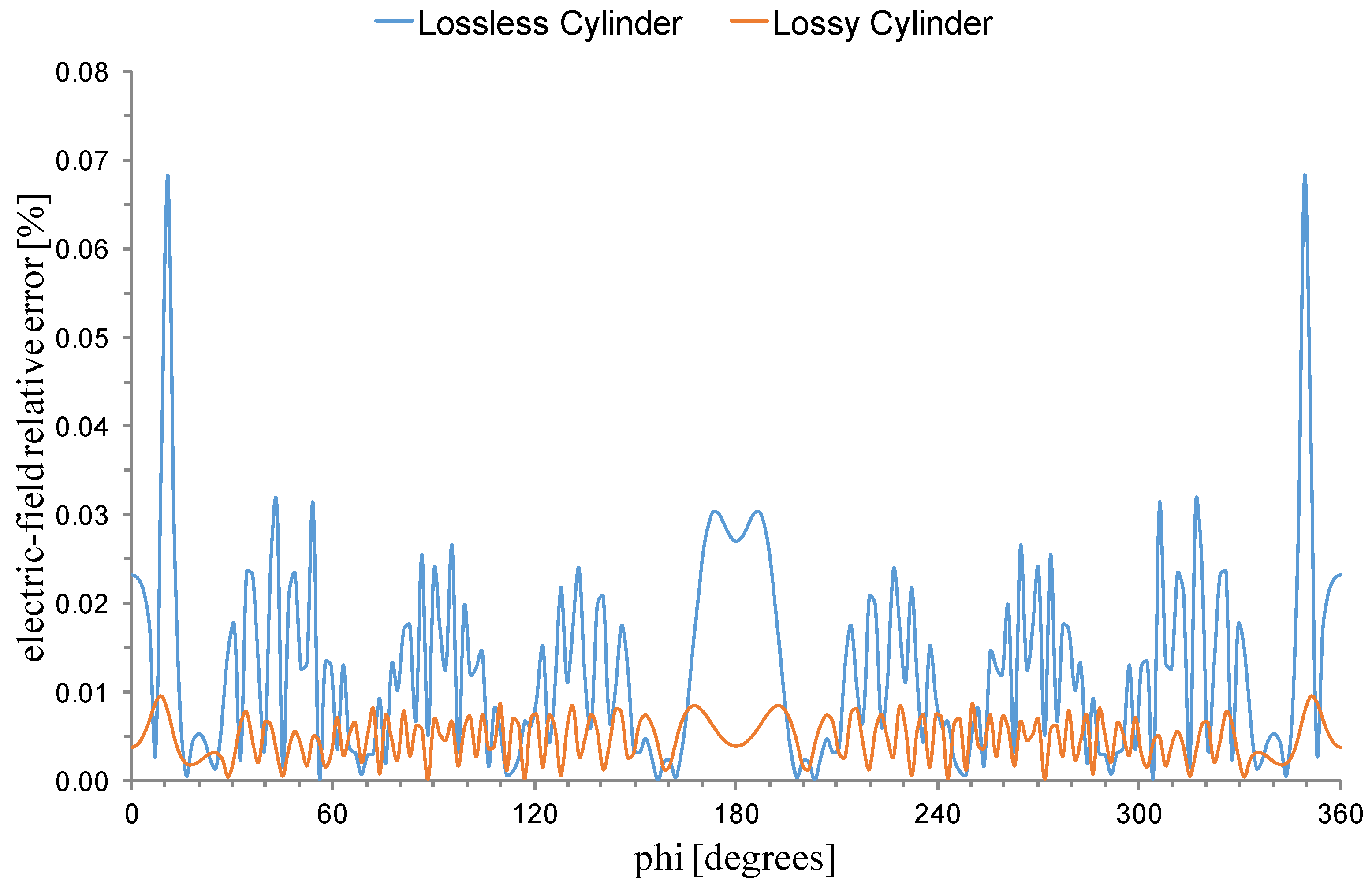
| 1 × 1 lattice | GHz m | 0.023 | 0.154 | 0.007 | 0.059 |
| 1 × 1 lattice | GHz m | 0.029 | 0.253 | 0.010 | 0.087 |
| 1 × 5 lattice | GHz | 0.023 | 0.152 | 0.007 | 0.057 |
| 5 × 5 lattice | GHz
m m | 0.027 | 0.189 | 0.005 | 0.039 |
Publisher’s Note: MDPI stays neutral with regard to jurisdictional claims in published maps and institutional affiliations. |
© 2022 by the authors. Licensee MDPI, Basel, Switzerland. This article is an open access article distributed under the terms and conditions of the Creative Commons Attribution (CC BY) license (https://creativecommons.org/licenses/by/4.0/).
Share and Cite
Mastorakis, E.; Papakanellos, P.J.; Anastassiu, H.T.; Tsitsas, N.L. Analysis of Electromagnetic Scattering from Large Arrays of Cylinders via a Hybrid of the Method of Auxiliary Sources (MAS) with the Fast Multipole Method (FMM). Mathematics 2022, 10, 3211. https://doi.org/10.3390/math10173211
Mastorakis E, Papakanellos PJ, Anastassiu HT, Tsitsas NL. Analysis of Electromagnetic Scattering from Large Arrays of Cylinders via a Hybrid of the Method of Auxiliary Sources (MAS) with the Fast Multipole Method (FMM). Mathematics. 2022; 10(17):3211. https://doi.org/10.3390/math10173211
Chicago/Turabian StyleMastorakis, Eleftherios, Panagiotis J. Papakanellos, Hristos T. Anastassiu, and Nikolaos L. Tsitsas. 2022. "Analysis of Electromagnetic Scattering from Large Arrays of Cylinders via a Hybrid of the Method of Auxiliary Sources (MAS) with the Fast Multipole Method (FMM)" Mathematics 10, no. 17: 3211. https://doi.org/10.3390/math10173211
APA StyleMastorakis, E., Papakanellos, P. J., Anastassiu, H. T., & Tsitsas, N. L. (2022). Analysis of Electromagnetic Scattering from Large Arrays of Cylinders via a Hybrid of the Method of Auxiliary Sources (MAS) with the Fast Multipole Method (FMM). Mathematics, 10(17), 3211. https://doi.org/10.3390/math10173211