
Binarization Technique Comparisons of Swarm Intelligence Algorithm: An Application to the Multi-Demand Multidimensional Knapsack Problem


Abstract
:1. Introduction
- The MDMKP is solved through hybrid techniques that integrate unsupervised learning techniques and swarm intelligence algorithms.
- The k-means binarization operator is compared to random and percentile operators to determine its contribution.
- A repair operator is proposed to Fix invalid solutions.
2. The Multi-Demand Multidimensional Knapsack Problem
3. The Machine Learning Swarm Intelligence Algorithm
3.1. Initialization Operator
| Algorithm 1: The initialization operator. |
|
3.2. ML Binary Operator
| Algorithm 2: The ML Binary operator (MLB). |
|
3.3. Repair Operator and Local Search Operator
| Algorithm 3: The repair operator. |
|
4. Results
4.1. Parameter Setting
- The difference between the best value achieved and the best known value:
- The difference between the worst value achieved and the best value known:
- The departure of the obtained average value from the best-known value:
- The convergence time used in the execution:
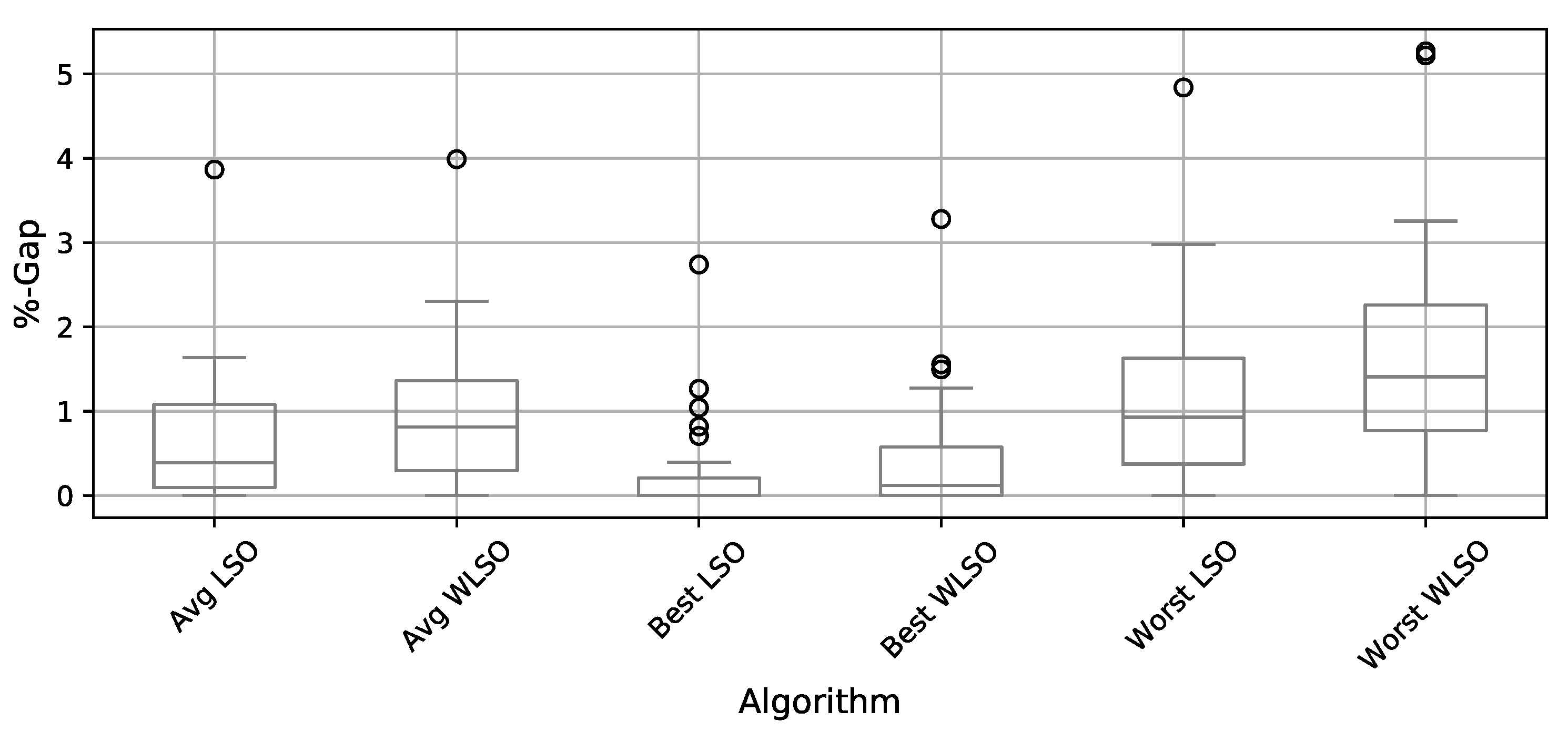
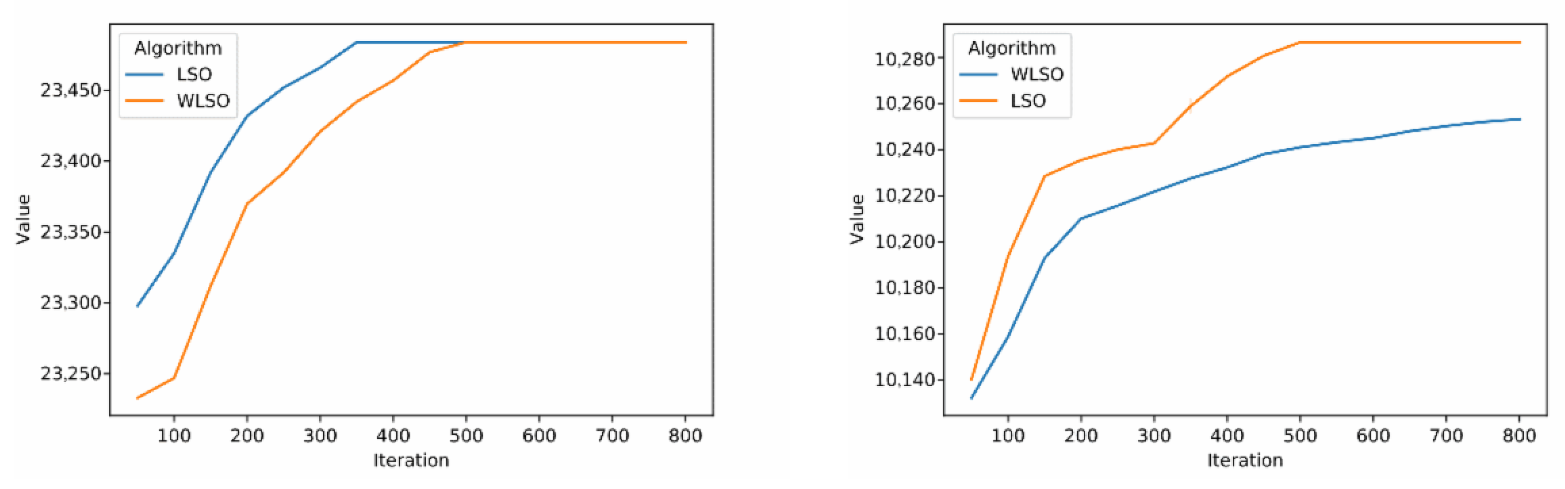
4.2. Local Search Operator Contribution
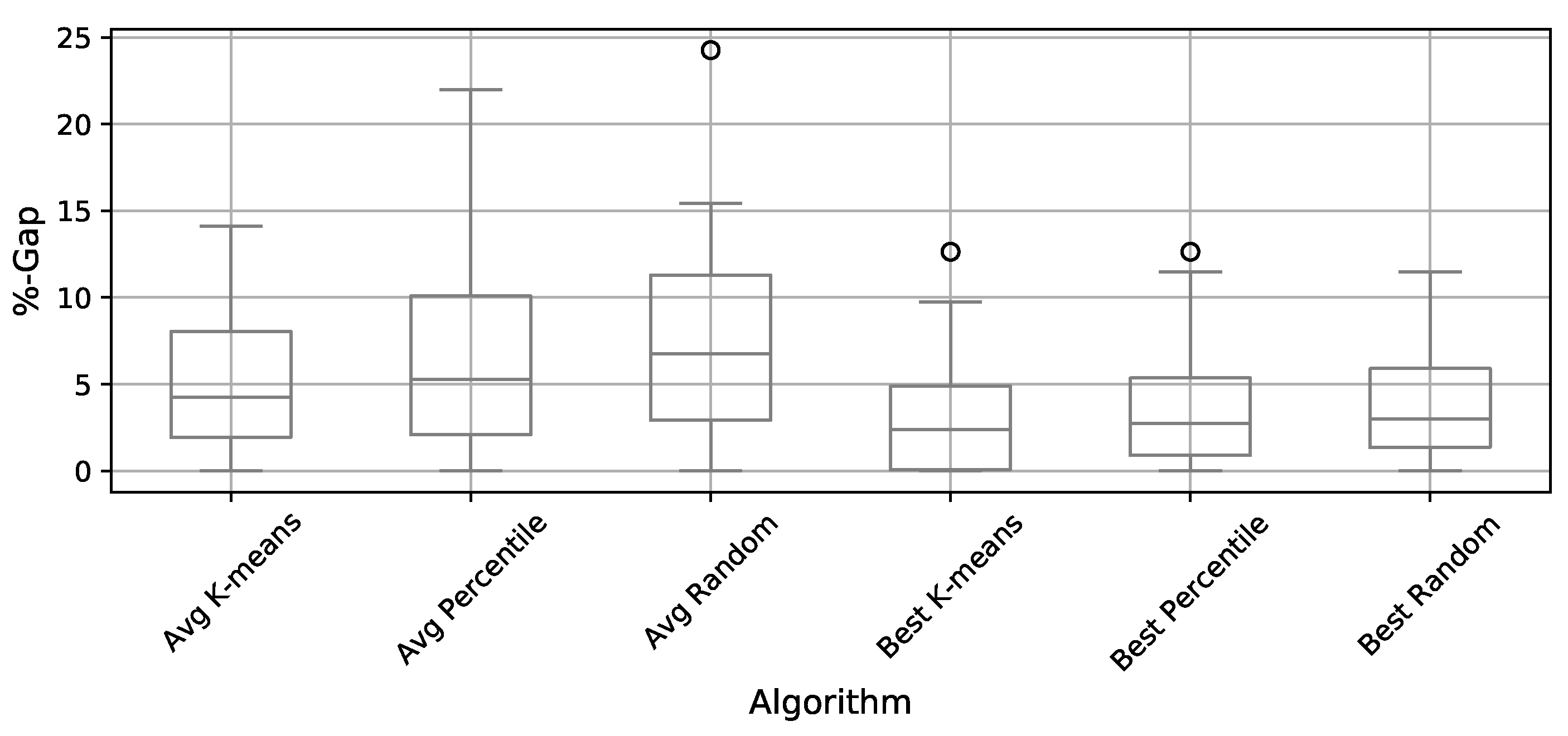
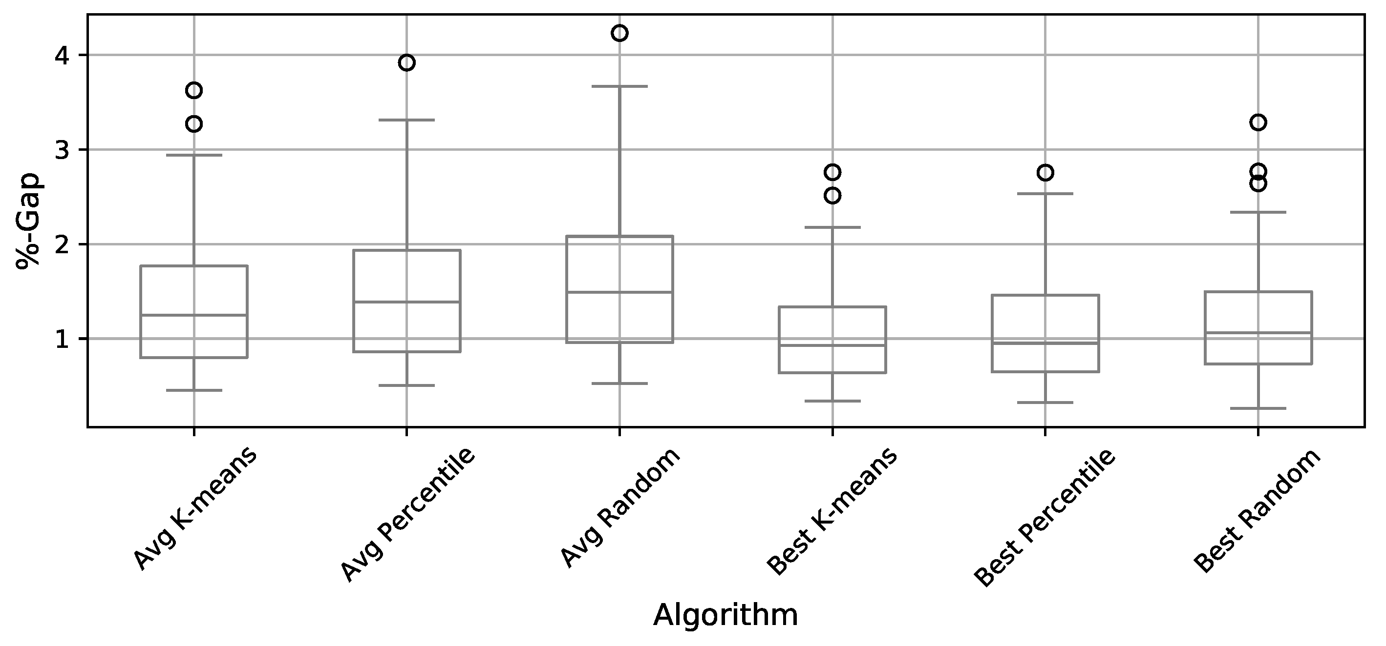
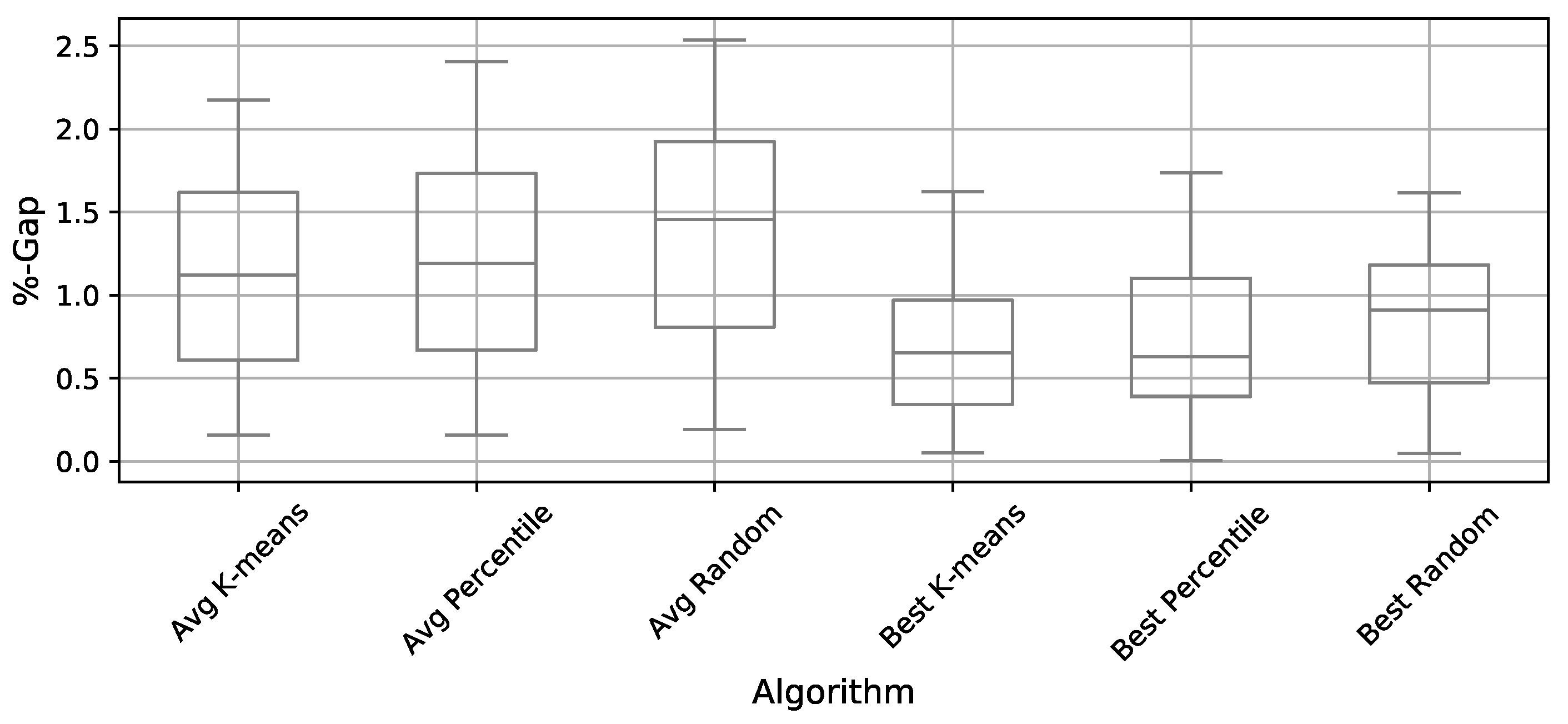
4.3. Comparison of Binarization Methods
5. Conclusions
Author Contributions
Funding
Institutional Review Board Statement
Informed Consent Statement
Data Availability Statement
Conflicts of Interest
References
- Abualigah, L.; Elaziz, M.A.; Khasawneh, A.M.; Alshinwan, M.; Ibrahim, R.A.; Al-qaness, M.A.; Mirjalili, S.; Sumari, P.; Gandomi, A.H. Meta-heuristic optimization algorithms for solving real-world mechanical engineering design problems: A comprehensive survey, applications, comparative analysis, and results. Neural Comput. Appl. 2022, 34, 4081–4110. [Google Scholar] [CrossRef]
- Chaharmahali, G.; Ghandalipour, D.; Jasemi, M.; Molla-Alizadeh-Zavardehi, S. Modified metaheuristic algorithms to design a closed-loop supply chain network considering quantity discount and fixed-charge transportation. Expert Syst. Appl. 2022, 202, 117364. [Google Scholar] [CrossRef]
- Penadés-Plà, V.; García-Segura, T.; Yepes, V. Robust design optimization for low-cost concrete box-girder bridge. Mathematics 2020, 8, 398. [Google Scholar] [CrossRef]
- García, J.; Lemus-Romani, J.; Altimiras, F.; Crawford, B.; Soto, R.; Becerra-Rozas, M.; Moraga, P.; Becerra, A.P.; Fritz, A.P.; Rubio, J.M.; et al. A binary machine learning cuckoo search algorithm improved by a local search operator for the set-union knapsack problem. Mathematics 2021, 9, 2611. [Google Scholar] [CrossRef]
- Wolpert, D.H.; Macready, W.G. No free lunch theorems for optimization. IEEE Trans. Evol. Comput. 1997, 1, 67–82. [Google Scholar] [CrossRef]
- Kareem, S.S.; Mostafa, R.R.; Hashim, F.A.; El-Bakry, H.M. An effective feature selection model using hybrid metaheuristic algorithms for iot intrusion detection. Sensors 2022, 22, 1396. [Google Scholar] [CrossRef]
- Yadav, R.K.; Mahapatra, R.P. Hybrid metaheuristic algorithm for optimal cluster head selection in wireless sensor network. Pervasive Mob. Comput. 2022, 79, 101504. [Google Scholar] [CrossRef]
- Roshani, M.; Phan, G.; Roshani, G.H.; Hanus, R.; Nazemi, B.; Corniani, E.; Nazemi, E. Combination of X-ray tube and GMDH neural network as a nondestructive and potential technique for measuring characteristics of gas-oil–water three phase flows. Measurement 2021, 168, 108427. [Google Scholar] [CrossRef]
- Roshani, S.; Jamshidi, M.B.; Mohebi, F.; Roshani, S. Design and Modeling of a Compact Power Divider with Squared Resonators Using Artificial Intelligence. Wirel. Pers. Commun. 2021, 117, 2085–2096. [Google Scholar] [CrossRef]
- Talbi, E.G. Machine Learning into Metaheuristics: A Survey and Taxonomy. ACM Comput. Surv. (CSUR) 2021, 54, 1–32. [Google Scholar] [CrossRef]
- Calvet, L.; de Armas, J.; Masip, D.; Juan, A.A. Learnheuristics: Hybridizing metaheuristics with machine learning for optimization with dynamic inputs. Open Math. 2017, 15, 261–280. [Google Scholar] [CrossRef]
- Crawford, B.; Soto, R.; Astorga, G.; García, J.; Castro, C.; Paredes, F. Putting continuous metaheuristics to work in binary search spaces. Complexity 2017, 2017, 8404231. [Google Scholar] [CrossRef]
- García, J.; Astorga, G.; Yepes, V. An analysis of a KNN perturbation operator: An application to the binarization of continuous metaheuristics. Mathematics 2021, 9, 225. [Google Scholar] [CrossRef]
- García, J.; Martí, J.V.; Yepes, V. The buttressed walls problem: An application of a hybrid clustering particle swarm optimization algorithm. Mathematics 2020, 8, 862. [Google Scholar] [CrossRef]
- García, J.; Crawford, B.; Soto, R.; Castro, C.; Paredes, F. A k-means binarization framework applied to multidimensional knapsack problem. Appl. Intell. 2018, 48, 357–380. [Google Scholar] [CrossRef]
- Mirjalili, S. SCA: A sine cosine algorithm for solving optimization problems. Knowl.-Based Syst. 2016, 96, 120–133. [Google Scholar] [CrossRef]
- Yang, X.S.; Deb, S. Engineering optimisation by cuckoo search. Int. J. Math. Model. Numer. Optim. 2010, 1, 330–343. [Google Scholar] [CrossRef]
- Lai, X.; Hao, J.K.; Yue, D. Two-stage solution-based tabu search for the multidemand multidimensional knapsack problem. Eur. J. Oper. Res. 2019, 274, 35–48. [Google Scholar] [CrossRef]
- Song, M.S.; Emerick, B.; Lu, Y.; Vasko, F.J. When to use Integer Programming Software to solve large multi-demand multidimensional knapsack problems: A guide for operations research practitioners. Eng. Optim. 2022, 54, 894–906. [Google Scholar] [CrossRef]
- Cappanera, P.; Trubian, M. A local-search-based heuristic for the demand-constrained multidimensional knapsack problem. Informs J. Comput. 2005, 17, 82–98. [Google Scholar] [CrossRef] [Green Version]
- Arntzen, H.; Hvattum, L.M.; Løkketangen, A. Adaptive memory search for multidemand multidimensional knapsack problems. Comput. Oper. Res. 2006, 33, 2508–2525. [Google Scholar] [CrossRef]
- Gortazar, F.; Duarte, A.; Laguna, M.; Martí, R. Black box scatter search for general classes of binary optimization problems. Comput. Oper. Res. 2010, 37, 1977–1986. [Google Scholar] [CrossRef]
- Cappanera, P.; Gallo, G.; Maffioli, F. Discrete facility location and routing of obnoxious activities. Discret. Appl. Math. 2003, 133, 3–28. [Google Scholar] [CrossRef]
- Beaujon, G.J.; Marin, S.P.; McDonald, G.C. Balancing and optimizing a portfolio of R&D projects. Nav. Res. Logist. (NRL) 2001, 48, 18–40. [Google Scholar]
- Wilcoxon, F. Individual comparisons by ranking methods. In Breakthroughs in Statistics; Springer: New York, NY, USA, 1992; pp. 196–202. [Google Scholar]
- Lam, S.K.; Pitrou, A.; Seibert, S. Numba: A llvm-based python jit compiler. In Proceedings of the Second Workshop on the LLVM Compiler Infrastructure in HPC, Austin, TX, USA, 15 November 2015; pp. 1–6. [Google Scholar]
- García, J.; Moraga, P.; Valenzuela, M.; Pinto, H. A db-scan hybrid algorithm: An application to the multidimensional knapsack problem. Mathematics 2020, 8, 507. [Google Scholar] [CrossRef]
- Valenzuela, M.; Peña, A.; Lopez, L.; Pinto, H. A binary multi-verse optimizer algorithm applied to the set covering problem. In Proceedings of the 2017 4th International Conference on Systems and Informatics (ICSAI), Hangzhou, China, 11–13 November 2017; IEEE: Piscataway, NJ, USA, 2017; pp. 513–518. [Google Scholar]
- García, J.; Lalla Ruiz, E.; Voß, S.; Lopez Droguett, E. Enhancing a machine learning binarization framework by perturbation operators: Analysis on the multidimensional knapsack problem. Int. J. Mach. Learn. Cybern. 2020, 11, 1951–1970. [Google Scholar] [CrossRef]


| Parameter | Description | Used Value | Explored Range |
|---|---|---|---|
| P | Particle number | 5 | [5, 10, 20] |
| K | Number of groups | 5 | [4, 5, 6] |
| I | Swarm iterations | 800 | [600, 800, 1000, 1200] |
| L | Local search iterations | 2000 | [1000, 2000, 4000] |
| LSO | WLSO | ||||||||||
|---|---|---|---|---|---|---|---|---|---|---|---|
| Instance | Best Known | Best | Avg. | Worst | Std. | Time(s) | Best | Avg. | Worst | Std. | Time(s) |
| 100-5-2-0-0 | 28,384 | 28,384 | 28,330.8 | 28,223 | 49.4 | 2.7 | 28,330 | 28,312.1 | 28,185 | 52.1 | 2.4 |
| 100-5-2-0-1 | 26,386 | 26,386 | 26,335.6 | 26,196 | 70.9 | 2.5 | 26,318 | 26,307.3 | 26,182 | 75.4 | 2.1 |
| 100-5-2-0-2 | 23,484 | 23,484 | 23,484.0 | 23,484 | 0.0 | 1.5 | 23,484 | 23,484 | 23,484 | 0.0 | 2.7 |
| 100-5-2-0-3 | 27,374 | 27,374 | 27,301.1 | 27,267 | 20.6 | 1.9 | 27,298 | 27,264.6 | 27,154 | 18.4 | 2.3 |
| 100-5-2-0-4 | 30,632 | 30,632 | 30,619.2 | 30,594 | 16.6 | 2.7 | 30,632 | 30,597.4 | 30,505 | 24.2 | 2.4 |
| 100-5-2-0-5 | 44,674 | 44,614 | 44,589.2 | 44,526 | 31.6 | 3.3 | 44,593 | 44,543.1 | 44,351 | 37.8 | 3.1 |
| 100-5-2-1-0 | 10,379 | 10,364 | 10,286.6 | 10,249 | 28.6 | 2.8 | 10,364 | 10,253.2 | 10,232 | 32.1 | 4.1 |
| 100-5-2-1-1 | 11,114 | 11,114 | 11,114.0 | 11,114 | 0.0 | 1.0 | 11,114 | 11,114 | 11,114 | 0.0 | 0.9 |
| 100-5-2-1-2 | 10,124 | 10,084 | 9998.0 | 9939 | 37 | 3.6 | 10,066 | 9956.4 | 9870 | 41.2 | 3.8 |
| 100-5-2-1-3 | 10,567 | 10,567 | 10,561.7 | 10,559 | 3.8 | 2.0 | 10,559 | 10,541.3 | 10,487 | 14.5 | 1.6 |
| 100-5-2-1-4 | 10,658 | 10,547 | 10,523.5 | 10,485 | 17.4 | 2.2 | 10,522 | 10,512.1 | 10,466 | 23.7 | 2.1 |
| 100-5-2-1-5 | 17,550 | 17,545 | 17,520.3 | 17,470 | 19.4 | 3.1 | 17,545 | 17,503.6 | 17,425 | 24.6 | 2.9 |
| 100-5-5-0-0 | 21,892 | 21,892 | 21,886.9 | 21,740 | 27.8 | 2.2 | 21,892 | 21,832.1 | 21,642 | 57.3 | 2.1 |
| 100-5-5-0-1 | 26,280 | 26,280 | 26,280.0 | 26,280 | 0.0 | 1.1 | 26,280 | 26,237.2 | 26,152 | 21.5 | 1.5 |
| 100-5-5-0-2 | 20,628 | 20,628 | 20,628.0 | 20,628 | 0.0 | 0.6 | 20,628 | 20,601.5 | 20,584 | 12.5 | 1.1 |
| 100-5-5-0-3 | 21,547 | 21,547 | 21,536.3 | 21,519 | 11.0 | 3.5 | 21,526 | 21,494.2 | 21,448 | 28.7 | 2.8 |
| 100-5-5-0-4 | 25,074 | 25,074 | 25,067.9 | 25,067 | 2.4 | 3.4 | 25,067 | 25,045.1 | 24,957 | 11.3 | 2.6 |
| 100-5-5-0-5 | 40,327 | 40,327 | 40,258.9 | 40,175 | 36.5 | 4.1 | 40,299 | 40,206.3 | 39,947 | 53.2 | 3.6 |
| 100-5-5-1-0 | 10,263 | 10,263 | 10,221.7 | 10,148 | 39.8 | 2.4 | 10,263 | 10,113.1 | 9929 | 56.7 | 2.3 |
| 100-5-5-1-1 | 10,625 | 10,625 | 10,625.0 | 10,625 | 0.0 | 1.1 | 10,625 | 10,517 | 10,463 | 21.5 | 1.8 |
| 100-5-5-1-2 | 10,198 | 10,126 | 10,084.2 | 10,003 | 45.2 | 2.7 | 10,126 | 10,055.5 | 9951 | 54.7 | 2.4 |
| 100-5-5-1-3 | 10,030 | 9998 | 9921.6 | 9880 | 48.4 | 2.1 | 9880 | 9805.1 | 9755 | 67.8 | 2.3 |
| 100-5-5-1-4 | 9964 | 9838 | 9817.3 | 9780 | 20.7 | 3.1 | 9809 | 9790.8 | 9741 | 22.5 | 2.8 |
| 100-5-5-1-5 | 15,603 | 15,603 | 15,580.7 | 15,523 | 19.9 | 2.9 | 15,603 | 15,557.3 | 15,482 | 23.1 | 3.0 |
| 100-10-5-0-0 | 21,852 | 21,791 | 21,721.5 | 21,715 | 19.6 | 2.4 | 21,736 | 21,683.2 | 21,628 | 20.5 | 2.3 |
| 100-10-5-0-1 | 20,645 | 20,593 | 20,422.3 | 20,256 | 73.2 | 4.5 | 20,593 | 20,364.7 | 20,211 | 89.2 | 3.9 |
| 100-10-5-0-2 | 19,517 | 19,517 | 19,402.1 | 19,262 | 89.0 | 3.0 | 19,517 | 19,317.6 | 19,174 | 95.3 | 2.7 |
| 100-10-5-0-3 | 20,596 | 20,519 | 20,450.0 | 20,356 | 41.3 | 3.7 | 20,491 | 20,414.6 | 20,332 | 44.5 | 3.6 |
| 100-10-5-0-4 | 19,423 | 19,264 | 19,155.9 | 19,003 | 67.3 | 3.9 | 19,264 | 19,122.8 | 18,950 | 75.4 | 3.8 |
| 100-10-5-0-5 | 35,933 | 35,859 | 35,642.6 | 35,517 | 82.7 | 5.3 | 35,727 | 35,594.3 | 35,445 | 74.3 | 4.5 |
| 100-10-5-1-0 | 10,018 | 10,018 | 9881.4 | 9789 | 65.9 | 3.3 | 9955 | 9798.1 | 9749 | 69.2 | 3.2 |
| 100-10-5-1-1 | 9839 | 9839 | 9709.8 | 9678 | 51.8 | 2.3 | 9839 | 9701.3 | 9652 | 62.8 | 2.4 |
| 100-10-5-1-2 | 10,000 | 9726 | 9613.4 | 9516 | 55.4 | 2.9 | 9672 | 9601.1 | 9478 | 82.5 | 2.8 |
| 100-10-5-1-3 | 10,544 | 10,544 | 10,468.0 | 10,388 | 59.8 | 3.6 | 10,544 | 10,453.2 | 10,306 | 66.8 | 3.4 |
| 100-10-5-1-4 | 10,011 | 10,011 | 9871.7 | 9739 | 48.6 | 2.8 | 9904 | 9822.4 | 9699 | 54.3 | 2.7 |
| 100-10-5-1-5 | 16,230 | 16,196 | 16,051.0 | 15,938 | 80.1 | 4.4 | 16,084 | 16,034.7 | 15,860 | 101.3 | 4.1 |
| 100-10-10-0-0 | 22,054 | 22,054 | 21,943.1 | 21,841 | 55.5 | 5.2 | 21,952 | 21,922.4 | 21,824 | 58.6 | 4.8 |
| 100-10-10-0-1 | 20,103 | 20,103 | 20,103.0 | 20,103 | 0.0 | 1.2 | 20,103 | 20,009 | 19,947 | 48.6 | 1.1 |
| 100-10-10-0-2 | 19,381 | 19,381 | 19,238.8 | 19,112 | 90.0 | 5.6 | 19,381 | 19,201.4 | 19,030 | 104.5 | 4.5 |
| 100-10-10-0-3 | 17,434 | 17,434 | 17,386.2 | 17,372 | 21.5 | 3.8 | 17,434 | 17,324.9 | 17,256 | 45.6 | 3.9 |
| 100-10-10-0-4 | 18,792 | 18,792 | 18,704.1 | 18,625 | 50.7 | 4.2 | 18,716 | 18,632.5 | 18,464 | 51.5 | 4.1 |
| 100-10-10-0-5 | 33,837 | 33,740 | 33,701.5 | 33,642 | 34.6 | 5.2 | 33,740 | 33,672.3 | 33,596 | 43.7 | 5.0 |
| 100-10-10-1-0 | 8560 | 8560 | 8420.1 | 8305 | 68.6 | 3.7 | 8475 | 8363.0 | 8109 | 66.3 | 3.9 |
| 100-10-10-1-1 | 8493 | 8493 | 8491.2 | 8439 | 9.9 | 2.6 | 8493 | 8464.8 | 8300 | 24.5 | 2.3 |
| 100-10-10-1-2 | 9266 | 9266 | 9231.5 | 9157 | 26.1 | 3.8 | 9266 | 9202.8 | 9010 | 41.2 | 3.6 |
| 100-10-10-1-3 | 9823 | 9823 | 9809.6 | 9622 | 51.0 | 3.4 | 9823 | 9721.4 | 9602 | 74.8 | 3.1 |
| 100-10-10-1-4 | 8929 | 8929 | 8919.4 | 8812 | 26.7 | 3.7 | 8872 | 8843.2 | 8771 | 38.4 | 3.5 |
| 100-10-10-1-5 | 14,152 | 14,151 | 14,102.9 | 14,054 | 26.4 | 4.4 | 14,151 | 14,083.1 | 13,954 | 35.2 | 4.3 |
| average | 18,108 | 18,081 | 18,021.1 | 17,952 | 36.3 | 3.1 | 18,053 | 17,979.6 | 17,871 | 46.8 | 3.0 |
| p-value | |||||||||||
| Instance | Random | Percentile | k-Means | |||||||||||||
|---|---|---|---|---|---|---|---|---|---|---|---|---|---|---|---|---|
| Best Known | Best | Average | Worst | Std. | Time(s) | Best | Average | Worst | Std. | Time(s) | Best | Average | Worst | Std. | Time(s) | |
| 250-5-2-0-0 | 78,486 | 77,896 | 77,598.9 | 77,014 | 225.7 | 16.8 | 78,166 | 77,986.8 | 77,727 | 123.4 | 20.88 | 78,279 | 78,091.7 | 77,941 | 82.5 | 23.2 |
| 250-5-2-0-1 | 75,132 | 74,658 | 73,966.9 | 72,845 | 390.6 | 16.8 | 74,887 | 74,587.4 | 73,929 | 237.1 | 21.96 | 74,989 | 74,689.6 | 74,228 | 193.4 | 21.4 |
| 250-5-2-0-2 | 71,003 | 70,112 | 69,404 | 68,024 | 432 | 19.6 | 70,602 | 70,281.6 | 69,808 | 225.5 | 21.84 | 70,698 | 70,489.4 | 70,166 | 134.3 | 24 |
| 250-5-2-0-3 | 80,311 | 80,014 | 79,862.6 | 79,671 | 82.2 | 16.5 | 80,145 | 79,953.9 | 79,840 | 65.2 | 11.52 | 80,165 | 79,979.2 | 79,875 | 61.8 | 17.5 |
| 250-5-2-0-4 | 70,935 | 70,613 | 70,458.7 | 70,244 | 90.3 | 14.0 | 70,814 | 70,575.2 | 70,411 | 91.7 | 13.8 | 70,757 | 70,601.4 | 70,518 | 50.5 | 28 |
| 250-5-2-0-5 | 130,981 | 129,154 | 128,414.9 | 127,313 | 474.2 | 33.3 | 129,883 | 128,713 | 128,006 | 463.8 | 24.36 | 129,883 | 129,090.3 | 128,100 | 386 | 27.5 |
| 250-5-2-1-0 | 26,666 | 26,361 | 26,270.7 | 26,148 | 62 | 21.6 | 26,446 | 26,325.2 | 26,248 | 47.6 | 16.08 | 26,465 | 26,360.7 | 26,301 | 43.4 | 15.8 |
| 250-5-2-1-1 | 26,864 | 26,619 | 26,505.7 | 26,411 | 48.1 | 18.8 | 26,700 | 26,556.1 | 26,447 | 51.4 | 14.64 | 26,661 | 26,565.2 | 26,501 | 38 | 14 |
| 250-5-2-1-2 | 27,280 | 27,018 | 26,914 | 26,815 | 53.2 | 19.9 | 27,131 | 26,966.1 | 26,854 | 60.9 | 13.44 | 27,152 | 26,992.5 | 26,888 | 57.6 | 16 |
| 250-5-2-1-3 | 26,269 | 26,008 | 25,888.8 | 25,786 | 55.7 | 21.8 | 26,056 | 25,915 | 25,832 | 54.4 | 11.76 | 26,019 | 25,941.7 | 25,853 | 46.2 | 16.7 |
| 250-5-2-1-4 | 27,293 | 27,023 | 26,948.3 | 26,877 | 40.4 | 21.3 | 27,122 | 27,005.7 | 26,885 | 62.3 | 15.36 | 27,121 | 27,016.9 | 26,950 | 46.4 | 17.7 |
| 250-5-2-1-5 | 44,395 | 44,192 | 44,054.6 | 43,865 | 68.7 | 23.8 | 44,203 | 44,081.1 | 43,944 | 72.7 | 15.72 | 44,219 | 44,122.2 | 44,014 | 48.3 | 21.2 |
| 250-5-5-0-0 | 68,026 | 67,977 | 67,859.1 | 67,693 | 64.3 | 29.1 | 68,024 | 67,907.9 | 67,794 | 51.6 | 18.72 | 67,992 | 67,917.8 | 67,837 | 38.8 | 23.4 |
| 250-5-5-0-1 | 60,795 | 60,506 | 60,314.4 | 59,993 | 106.8 | 30.2 | 60,535 | 60,391.3 | 60,140 | 92 | 23.16 | 60,566 | 60,453 | 60,113 | 91.7 | 26.9 |
| 250-5-5-0-2 | 62,093 | 62,054 | 61,933.7 | 61,769 | 56.5 | 27.4 | 62,051 | 61,957.8 | 61,892 | 43.9 | 15.48 | 62,051 | 61,979.7 | 61,919 | 41.6 | 19.5 |
| 250-5-5-0-3 | 66,567 | 66,455 | 66,322.7 | 66,150 | 82.1 | 27.4 | 66,475 | 66,371 | 66,295 | 51.3 | 19.56 | 66,512 | 66,401.5 | 66,327 | 44.6 | 22.1 |
| 250-5-5-0-4 | 61,929 | 61,900 | 61,810.1 | 61,690 | 45.1 | 23.5 | 61,883 | 61,831.7 | 61,758 | 40 | 18.24 | 61,883 | 61,828.4 | 61,763 | 36 | 15.1 |
| 250-5-5-0-5 | 127,934 | 127,573 | 127,136.1 | 126,433 | 352 | 38.6 | 127,749 | 127,394.1 | 126,920 | 235.6 | 29.16 | 127,843 | 127,528.8 | 127,211 | 152 | 37.4 |
| 250-5-5-1-0 | 26,973 | 26,735 | 26,583.8 | 26,471 | 63.2 | 19.6 | 26,731 | 26,597.6 | 26,480 | 54.9 | 12.24 | 26,755 | 26,628.7 | 26,526 | 51.2 | 26.6 |
| 250-5-5-1-1 | 26,665 | 26,415 | 26,220.1 | 25,998 | 84.9 | 24.4 | 26,376 | 26,237.1 | 26,136 | 63.5 | 18 | 26,400 | 26,269.8 | 26,167 | 64 | 16.5 |
| 250-5-5-1-2 | 26,648 | 26,405 | 26,135.4 | 26,004 | 81.8 | 21.0 | 26,324 | 26,167.5 | 26,052 | 67.7 | 14.04 | 26,310 | 26,182.3 | 26,103 | 51.3 | 17 |
| 250-5-5-1-3 | 25,923 | 25,585 | 25,418.1 | 25,324 | 63.6 | 21.8 | 25,602 | 25,442.2 | 25,334 | 60.4 | 15 | 25,544 | 25,437.8 | 25,335 | 53.8 | 23.1 |
| 250-5-5-1-4 | 26,060 | 25,722 | 25,553 | 25,416 | 76.6 | 22.1 | 25,670 | 25,563.8 | 25,469 | 51 | 17.52 | 25,717 | 25,585.3 | 25,464 | 58.5 | 17.7 |
| 250-5-5-1-5 | 41,372 | 40,878 | 40,712.1 | 40,628 | 49.3 | 27.4 | 40,940 | 40,765.7 | 40,640 | 74.6 | 20.64 | 41,024 | 40,784.5 | 40,639 | 83.3 | 23.7 |
| 250-10-5-0-0 | 56,306 | 55,655 | 55,321.6 | 54,974 | 188.3 | 34.4 | 55,989 | 55,593.8 | 55,206 | 178 | 44.28 | 55,989 | 55,574.4 | 54,950 | 211 | 34.2 |
| 250-10-5-0-1 | 59,619 | 59,498 | 59,182.5 | 58,932 | 118 | 38.4 | 59,359 | 59,227.5 | 59,076 | 67.1 | 28.2 | 59,520 | 59,267.7 | 59,141 | 84.8 | 27.8 |
| 250-10-5-0-2 | 54,898 | 54,398 | 54,094.7 | 53,651 | 194.4 | 40.3 | 54,620 | 54,250.8 | 53,834 | 166.6 | 30.6 | 54,525 | 54,277 | 53,948 | 132.9 | 32.9 |
| 250-10-5-0-3 | 52,399 | 51,873 | 51,574 | 51,191 | 180.8 | 37.8 | 51,882 | 51,662.2 | 51,434 | 95.6 | 27.48 | 51,912 | 51,745.1 | 51,539 | 99.7 | 35.9 |
| 250-10-5-0-4 | 58,234 | 57,561 | 56,984.1 | 56,528 | 282.9 | 38.6 | 57,470 | 57,209.4 | 56,781 | 102.4 | 29.64 | 57,694 | 57,365.4 | 57,038 | 139.5 | 32.4 |
| 250-10-5-0-5 | 99,682 | 99,002 | 98,572.4 | 98,139 | 232.7 | 45.4 | 99,052 | 98,751.3 | 98,424 | 145.6 | 36.24 | 99,074 | 98,761.8 | 98,421 | 148.5 | 42.4 |
| 250-10-5-1-0 | 26,961 | 26,533 | 26,401.2 | 26,261 | 67.9 | 30.0 | 26,630 | 26,449.4 | 26,330 | 69.1 | 18.96 | 26,560 | 26,436.7 | 26,343 | 46.9 | 23.4 |
| 250-10-5-1-1 | 26,658 | 26,346 | 26,170.7 | 26,068 | 63.6 | 27.4 | 26,373 | 26,227.7 | 26,109 | 64 | 22.32 | 26,299 | 26,213.6 | 26,106 | 49.8 | 25 |
| 250-10-5-1-2 | 25,737 | 25,357 | 25,138.5 | 24,973 | 86.7 | 27.2 | 25,290 | 25,153.8 | 25,044 | 73.1 | 21 | 25,403 | 25,176.7 | 25,072 | 66.7 | 23.2 |
| 250-10-5-1-3 | 27,162 | 26,842 | 26,637.8 | 26,526 | 74.6 | 28.3 | 26,847 | 26,672.3 | 26,561 | 69.7 | 18 | 26,856 | 26,706.6 | 26,610 | 54.4 | 26.9 |
| 250-10-5-1-4 | 26,816 | 26,485 | 26,313.1 | 26,159 | 64.6 | 25.2 | 26,482 | 26,350.3 | 26,254 | 54.1 | 17.4 | 26,495 | 26,378.8 | 26,282 | 60.6 | 17.3 |
| 250-10-5-1-5 | 46,244 | 45,936 | 45,798 | 45,558 | 77.6 | 33.6 | 46,012 | 45,825.6 | 45,700 | 60.3 | 18.96 | 46,012 | 45,829.8 | 45,745 | 65.9 | 25.8 |
| 250-10-10-0-0 | 52,441 | 52,054 | 51,866.9 | 51,671 | 98.5 | 43.4 | 52,263 | 52,000.5 | 51,763 | 92.3 | 27.84 | 52,263 | 51,978.5 | 51,822 | 66.7 | 37 |
| 250-10-10-0-1 | 53,745 | 53,474 | 53,363.7 | 53,252 | 57 | 37.2 | 53,587 | 53,384.2 | 53,295 | 61.4 | 24.24 | 53,610 | 53,405.9 | 53,305 | 62.9 | 37.9 |
| 250-10-10-0-2 | 46,927 | 46,551 | 46,326.2 | 46,163 | 79.3 | 37.8 | 46,506 | 46,360.4 | 46,207 | 76.2 | 26.16 | 46,545 | 46,422.6 | 46,291 | 71.9 | 31.7 |
| 250-10-10-0-3 | 54,831 | 54,592 | 54,384.9 | 54,176 | 96.2 | 41.4 | 54,676 | 54,481.7 | 54,343 | 73.8 | 29.04 | 54,598 | 54,492.2 | 54,363 | 67.1 | 38.8 |
| 250-10-10-0-4 | 49,675 | 49,442 | 49,230.9 | 48,963 | 105.7 | 38.6 | 49,356 | 49,259.2 | 48,981 | 71.8 | 28.92 | 49,419 | 49,287.5 | 49,188 | 55.6 | 56.8 |
| 250-10-10-0-5 | 92,975 | 92,559 | 92,374.1 | 92,024 | 131.5 | 51.5 | 92,676 | 92,461.5 | 92,280 | 64.5 | 28.56 | 92,658 | 92,526.3 | 92,384 | 66.4 | 52.2 |
| 250-10-10-1-0 | 26,696 | 26,447 | 26,300.9 | 26,188 | 67.6 | 28.3 | 26,537 | 26,315 | 26,175 | 69.9 | 20.4 | 26,537 | 26,318.7 | 26,216 | 60.9 | 26.9 |
| 250-10-10-1-1 | 25,876 | 25,543 | 25,336.9 | 25,185 | 85.4 | 31.9 | 25,564 | 25,388.5 | 25,265 | 69.9 | 18.96 | 25,627 | 25,431.1 | 25,317 | 70.6 | 27.5 |
| 250-10-10-1-2 | 26,517 | 26,134 | 25,975.7 | 25,883 | 67.1 | 28.0 | 26,271 | 26,026 | 25,892 | 76.5 | 23.76 | 26,192 | 26,049.1 | 25,848 | 80.4 | 27.8 |
| 250-10-10-1-3 | 26,684 | 26,271 | 26,006.9 | 25,816 | 93.3 | 33.6 | 26,258 | 26,041.6 | 25,879 | 91.6 | 19.92 | 26,251 | 26,113.8 | 26,005 | 64.4 | 21.3 |
| 250-10-10-1-4 | 26,676 | 26,245 | 26,123.5 | 25,971 | 74.9 | 29.7 | 26,358 | 26,170 | 26,017 | 81.3 | 21.24 | 26,467 | 26,233.9 | 26,099 | 79.7 | 27.7 |
| 250-10-10-1-5 | 42,629 | 42,248 | 41,888.9 | 41,688 | 142.5 | 37.2 | 42,093 | 41,939.8 | 41,823 | 76.2 | 30.48 | 42,122 | 41,940.5 | 41,777 | 95 | 33.5 |
| Average | 49,853.9 | 49,477.5 | 49,242.8 | 48,969.2 | 122.5 | 29.2 | 49,555.5 | 49,349.5 | 49,156.5 | 93.6 | 21.6 | 49,575.7 | 49,393.2 | 49,219.8 | 82.4 | 26.6 |
| p-value | ||||||||||||||||
| Instance | Random | Percentile | K-Means | |||||||||||||
|---|---|---|---|---|---|---|---|---|---|---|---|---|---|---|---|---|
| Best Known | Best | Average | Worst | Std. | Time(s) | Best | Average | Worst | Std. | Time(s) | Best | Average | Worst | Std. | Time(s) | |
| 100-30-30-0-2-1 | 11,312 | 10,762 | 10,497.3 | 10,310 | 130.6 | 10.2 | 10,832 | 10,622.3 | 10,447.0 | 141.6 | 11.8 | 11,038.0 | 10,696.0 | 10,447.0 | 177.9 | 15.4 |
| 100-30-30-0-2-2 | 9945 | 9945 | 9845.0 | 9785 | 75.6 | 8.0 | 9945 | 9867.7 | 9785.0 | 78.6 | 10.0 | 9945.0 | 9941.0 | 9905.0 | 12.2 | 16.2 |
| 100-30-30-0-2-3 | 11,195 | 10,437 | 10,392.7 | 10,051 | 116.5 | 13.3 | 10,494 | 10,440.8 | 10,437.0 | 14.3 | 14.2 | 10,494.0 | 10,438.9 | 10,437.0 | 10.4 | 8.6 |
| 100-30-30-0-2-4 | 11,324 | 10,426 | 10,319.8 | 10,162 | 60.4 | 10.8 | 10,557 | 10,363.9 | 10,182.0 | 89.7 | 19.0 | 10,778.0 | 10,466.4 | 10,325.0 | 102.9 | 13.3 |
| 100-30-30-0-2-5 | 9704 | 9704 | 9354.2 | 8943 | 317.0 | 12.7 | 9704 | 9684.9 | 9131.0 | 103.7 | 19.7 | 9704.0 | 9704.0 | 9704.0 | 0.0 | 10.7 |
| 100-30-30-0-2-6 | 23,296 | 22,504 | 22,297.2 | 22,131 | 114.5 | 11.9 | 22,705 | 22,427.2 | 22,170.0 | 170.0 | 16.1 | 22,705.0 | 22,439.5 | 22,186.0 | 115.6 | 16.9 |
| 100-30-30-0-2-7 | 22,442 | 21,890 | 21,491.3 | 21,232 | 128.8 | 13.2 | 21,780 | 21,514.0 | 21,343.0 | 107.5 | 13.5 | 21,784.0 | 21,604.5 | 21,462.0 | 92.7 | 17.6 |
| 100-30-30-0-2-8 | 23,452 | 22,778 | 22,655.3 | 22,497 | 87.3 | 12.9 | 22,908 | 22,694.1 | 22,515.0 | 93.3 | 17.2 | 22,908.0 | 22,724.8 | 22,562.0 | 87.3 | 12.1 |
| 100-30-30-0-2-9 | 22,756 | 22,348 | 21,736.8 | 21,523 | 175.4 | 15.0 | 22,491 | 21,846.8 | 21,631.0 | 210.7 | 21.1 | 22,500.0 | 21,942.1 | 21,620.0 | 210.0 | 20.6 |
| 100-30-30-0-2-10 | 24,371 | 24,042 | 23,613.2 | 23,447 | 133.0 | 11.4 | 24,042 | 23,707.6 | 23,482.0 | 132.5 | 17.6 | 24,135.0 | 23,750.9 | 23,528.0 | 142.7 | 17.1 |
| 100-30-30-0-2-11 | 33,472 | 33,472 | 33,472.0 | 33,472 | 0.0 | 22.5 | 33,472 | 33,472.0 | 33,472 | 0.0 | 23.3 | 33,472.0 | 33,472.0 | 33,472.0 | 0.0 | 18.2 |
| 100-30-30-0-2-12 | 32,670 | 32,200 | 32,031.3 | 31,959 | 112.3 | 4.9 | 32,200 | 32,035.4 | 31,763.0 | 123.5 | 5.5 | 32,200.0 | 32,068.5 | 31,959.0 | 114.1 | 4.6 |
| 100-30-30-0-2-13 | 32,942 | 32,228 | 32,015.6 | 31,931 | 103.3 | 13.2 | 32,942 | 32,106.0 | 31,931.0 | 198.9 | 16.5 | 32,942.0 | 32,199.9 | 31,942.0 | 167.5 | 19.3 |
| 100-30-30-0-2-14 | 35,106 | 34,823 | 34,615.2 | 34,505 | 105.8 | 13.9 | 34,823 | 34,689.8 | 34,511.0 | 103.0 | 16.7 | 34,986.0 | 34,780.8 | 34,572.0 | 117.0 | 13.7 |
| 100-30-30-0-2-15 | 30,930 | 30,456 | 30,445.1 | 30,292 | 41.6 | 3.1 | 30,555 | 30,472.5 | 30,456.0 | 37.2 | 6.0 | 30,678.0 | 30,532.9 | 30,456.0 | 75.1 | 11.4 |
| 100-30-30-1-5-1 | 5340 | 5158 | 4560.9 | 4168 | 243.1 | 8.6 | 5158 | 4760.1 | 4270.0 | 236.7 | 10.7 | 5158.0 | 4863.8 | 4636.0 | 204.7 | 10.9 |
| 100-30-30-1-5-2 | 4390 | 4114 | 3859.7 | 3337 | 273.6 | 7.7 | 4149 | 3923.9 | 3337.0 | 256.5 | 9.3 | 4149.0 | 4038.7 | 3623.0 | 170.4 | 14.6 |
| 100-30-30-1-5-3 | 4227 | 4227 | 3201.5 | 2877 | 213.6 | 13.1 | 4227 | 3298.4 | 3165.0 | 203.4 | 16.7 | 4227.0 | 3706.9 | 3256.0 | 406.8 | 16.8 |
| 100-30-30-1-5-4 | 4706 | 4166 | 4030.3 | 3620 | 173.5 | 14.3 | 4166 | 4108.2 | 3961.0 | 64.0 | 11.0 | 4407.0 | 4156.6 | 4103.0 | 72.8 | 13.1 |
| 100-30-30-1-5-5 | 2597 | 2597 | 2522.3 | 2373 | 107.4 | 8.4 | 2597 | 2597.0 | 2597 | 0.0 | 9.9 | 2597.0 | 2589.5 | 2373.0 | 40.9 | 6.6 |
| 100-30-30-1-5-6 | 10,808 | 10,145 | 9433.8 | 9069 | 236.6 | 12.7 | 10,145 | 9506.7 | 9069.0 | 241.6 | 20.6 | 10,021.0 | 9593.9 | 9341.0 | 141.2 | 15.4 |
| 100-30-30-1-5-7 | 9807 | 8989 | 8608.5 | 8201 | 194.6 | 12.1 | 9319 | 8731.0 | 8440.0 | 217.8 | 16.0 | 9319.0 | 8712.1 | 8354.0 | 219.4 | 16.3 |
| 100-30-30-1-5-8 | 10,882 | 10,314 | 9928.8 | 9369 | 301.2 | 12.1 | 10,346 | 10,071.2 | 9680.0 | 235.8 | 18.6 | 10,499.0 | 10,167.7 | 9709.0 | 227.4 | 13.8 |
| 100-30-30-1-5-9 | 10,595 | 9515 | 8961.4 | 8437 | 311.0 | 13.7 | 9256 | 8994.5 | 8583.0 | 230.5 | 17.2 | 9256.0 | 9100.4 | 8765.0 | 175.0 | 16.1 |
| 100-30-30-1-5-10 | 10,297 | 9155 | 8961.6 | 8693 | 116.7 | 11.9 | 9131 | 8961.6 | 8656.0 | 126.8 | 19.5 | 9293.0 | 9038.0 | 8819.0 | 133.1 | 16.5 |
| 100-30-30-1-5-11 | 11,029 | 11,029 | 11,029.0 | 11,029 | 0.0 | 29.0 | 11,029 | 11,029.0 | 11,029 | 0.0 | 24.0 | 11,029.0 | 11,029.0 | 11,029.0 | 0.0 | 14.9 |
| 100-30-30-1-5-12 | 11,884 | 11,296 | 11,045.5 | 10,859 | 128.2 | 10.6 | 11,360 | 11,174.9 | 11,044.0 | 97.8 | 17.6 | 11,681.0 | 11,273.5 | 11,213.0 | 119.0 | 15.2 |
| 100-30-30-1-5-13 | 10,751 | 10,431 | 10,039.7 | 9668 | 199.3 | 11.0 | 10,590 | 10,157.1 | 9732.0 | 142.6 | 15.8 | 10,751.0 | 10,273.1 | 10,126.0 | 172.2 | 13.6 |
| 100-30-30-1-5-14 | 11,567 | 10,998 | 10,537.2 | 10,156 | 170.8 | 12.7 | 10,847 | 10,594.5 | 10,453.0 | 119.0 | 16.7 | 10,998.0 | 10,635.4 | 10,453.0 | 130.7 | 13.1 |
| 100-30-30-1-5-15 | 10,671 | 10,351 | 9932.5 | 9836 | 177.4 | 9.9 | 10,351 | 10,135.8 | 9843.0 | 202.2 | 18.9 | 10,351.0 | 10,238.8 | 9843.0 | 179.2 | 13.4 |
| Average | 15,482.3 | 15,017 | 14,714.5 | 14,464.4 | 151.6 | 12.2 | 15,071 | 14,799.6 | 14,570.5 | 132.6 | 15.7 | 15,134 | 14,872.7 | 14,674.0 | 127.3 | 14.2 |
| p-value | 0.0022 | 0.0028 | 0.00078 | |||||||||||||
| Instance | Random | Percentile | K-Means | |||||||||||||
|---|---|---|---|---|---|---|---|---|---|---|---|---|---|---|---|---|
| Best Known | Best | Avg. | Worst | Std. | Time(s) | Best | Avg. | Worst | Std. | Time(s) | Best | Avg. | Worst | Std. | Time(s) | |
| 500-30-30-0-2-1 | 85,188 | 84,385 | 83,947.1 | 83,507 | 200.0 | 303.0 | 84,243 | 84,038.5 | 83,619 | 143.6 | 434.7 | 84,568 | 84,144.3 | 83,895 | 158.0 | 415.4 |
| 500-30-30-0-2-2 | 82,073 | 81,456 | 80,874.1 | 80,437 | 223.9 | 322.6 | 81,389 | 81,001.2 | 80,642 | 160.8 | 407.8 | 81,570 | 81,169.6 | 80,905 | 128.0 | 427.2 |
| 500-30-30-0-2-3 | 77,393 | 76,129 | 75,733.9 | 75,324 | 192.4 | 310.5 | 76,307 | 75,888.5 | 75,446 | 177.2 | 341.4 | 76,401 | 76,039.5 | 75,835 | 140.0 | 417.7 |
| 500-30-30-0-2-4 | 82,304 | 81,443 | 80,987.5 | 80,632 | 206.6 | 323.3 | 81,521 | 81,122.2 | 80,876 | 135.4 | 447.5 | 81,606 | 81,272.4 | 81,116 | 99.3 | 379.0 |
| 500-30-30-0-2-5 | 83,525 | 82,522 | 82,210.9 | 81,735 | 217.5 | 318.9 | 82,735 | 82,296.9 | 81,790 | 207.2 | 231.5 | 82,726 | 82,472.6 | 82,236 | 153.0 | 506.7 |
| 500-30-30-0-2-6 | 145,967 | 144,894 | 144,456.1 | 144,039 | 176.9 | 355.5 | 145,003 | 144,574.5 | 144,349 | 141.3 | 468.8 | 145,021 | 144,704.7 | 144,550 | 150.8 | 413.0 |
| 500-30-30-0-2-7 | 152,246 | 151,089 | 150,828.8 | 150,517 | 129.9 | 360.4 | 151,294 | 150,988.7 | 150,739 | 150.6 | 462.3 | 151,270 | 151,100.1 | 150,797 | 149.7 | 528.4 |
| 500-30-30-0-2-8 | 157,687 | 156,563 | 156,330.4 | 156,016 | 160.0 | 440.6 | 156,910 | 156,512.7 | 156,163 | 160.6 | 474.7 | 156,908 | 156,609.3 | 156,402 | 157.3 | 769.0 |
| 500-30-30-0-2-9 | 153,751 | 152,662 | 152,315.0 | 151,890 | 180.6 | 497.1 | 152,722 | 152,441.0 | 152,208 | 128.2 | 448.5 | 152,763 | 152,548.7 | 152,313 | 125.4 | 376.9 |
| 500-30-30-0-2-10 | 142,173 | 141,133 | 140,774.3 | 140,468 | 177.9 | 427.7 | 141,249 | 140,918.4 | 140,627 | 135.5 | 525.1 | 141,218 | 140,954.3 | 140,673 | 163.4 | 538.9 |
| 500-30-30-0-2-11 | 185,226 | 184,201 | 183,909.4 | 183,603 | 144.5 | 290.8 | 184,394 | 183,970.4 | 183,701 | 150.5 | 333.7 | 184,139 | 184,025.8 | 183,883 | 75.1 | 376.6 |
| 500-30-30-0-2-12 | 194,614 | 193,704 | 193,295.5 | 193,042 | 138.5 | 296.3 | 193,736 | 193,371.2 | 193,169 | 153.4 | 339.8 | 193,852 | 193,444.4 | 193,277 | 154.6 | 427.1 |
| 500-30-30-0-2-13 | 208,246 | 207,702 | 207,150.9 | 206,869 | 150.2 | 218.7 | 207,404 | 207,176.6 | 206,873 | 138.1 | 364.4 | 207,537 | 207,300.3 | 207,123 | 124.2 | 424.0 |
| 500-30-30-0-2-14 | 215,849 | 214,953 | 214,679.9 | 214,368 | 128.0 | 268.0 | 215,146 | 214,760.2 | 214,546 | 132.5 | 361.7 | 214,973 | 214,755.6 | 214,598 | 117.2 | 385.7 |
| 500-30-30-0-2-15 | 194,224 | 193,261 | 192,910.8 | 192,625 | 164.7 | 309.3 | 193,501 | 193,015.5 | 192,792 | 152.7 | 325.4 | 193,354 | 193,089.9 | 192,822 | 127.0 | 342.2 |
| 500-30-30-1-5-1 | 51,666 | 50,237 | 49,965.6 | 49,721 | 152.1 | 291.5 | 50,357 | 50,065.7 | 49,836 | 139.9 | 307.9 | 50,543 | 50,148.4 | 49,996 | 155.9 | 260.5 |
| 500-30-30-1-5-2 | 50,101 | 48,778 | 48,263.6 | 47,970 | 200.6 | 307.8 | 48,907 | 48,442.8 | 48,180 | 170.5 | 314.3 | 48,719 | 48,463.0 | 48,267 | 151.3 | 366.8 |
| 500-30-30-1-5-3 | 51,226 | 49,543 | 49,059.4 | 48,749 | 239.5 | 322.4 | 49,815 | 49,219.5 | 48,856 | 226.0 | 341.5 | 49,939 | 49,369.5 | 49,226 | 116.3 | 336.7 |
| 500-30-30-1-5-4 | 51,637 | 50,436 | 50,105.6 | 49,790 | 159.4 | 304.8 | 50,795 | 50,222.8 | 49,963 | 193.5 | 325.2 | 50,806 | 50,312.2 | 50,068 | 144.9 | 330.9 |
| 500-30-30-1-5-5 | 52,078 | 50,861 | 50,574.9 | 50,164 | 183.6 | 313.1 | 50,907 | 50,637.9 | 50,244 | 141.9 | 370.8 | 51,097 | 50,777.2 | 50,567 | 147.6 | 318.6 |
| 500-30-30-1-5-6 | 84,052 | 82,810 | 82,423.6 | 82,072 | 186.3 | 436.9 | 82,934 | 82,578.3 | 82,285 | 201.6 | 396.5 | 83,274 | 82,715.3 | 82,417 | 148.8 | 421.3 |
| 500-30-30-1-5-7 | 82,850 | 81,606 | 81,178.9 | 80,754 | 192.8 | 391.7 | 81,595 | 81,272.0 | 80,966 | 179.7 | 423.0 | 81,646 | 81,380.7 | 81,188 | 148.6 | 531.0 |
| 500-30-30-1-5-8 | 82,722 | 81,646 | 81,178.6 | 80,860 | 208.7 | 380.7 | 81,649 | 81,292.2 | 81,015 | 173.8 | 450.6 | 81,767 | 81,395.5 | 81,157 | 174.4 | 550.5 |
| 500-30-30-1-5-9 | 82,825 | 81,355 | 80,795.3 | 80,486 | 201.2 | 410.8 | 81,331 | 80,954.0 | 80,584 | 179.5 | 485.4 | 81,494 | 81,119.0 | 80,862 | 149.5 | 475.0 |
| 500-30-30-1-5-10 | 82,845 | 81,610 | 81,023.7 | 80,646 | 202.5 | 417.6 | 81,489 | 81,113.0 | 80,802 | 182.8 | 480.7 | 81,724 | 81,196.6 | 80,991 | 183.2 | 509.3 |
| 500-30-30-1-5-11 | 88,887 | 87,749 | 87,475.7 | 87,265 | 114.8 | 313.3 | 87,899 | 87,594.2 | 87,237 | 161.9 | 293.0 | 88,059 | 87,648.8 | 87,384 | 145.0 | 309.6 |
| 500-30-30-1-5-12 | 87,254 | 86,268 | 85,952.6 | 85,642 | 124.0 | 329.2 | 86,435 | 86,026.2 | 85,823 | 147.1 | 376.4 | 86,266 | 86,168.2 | 86,065 | 82.0 | 433.4 |
| 500-30-30-1-5-13 | 87,315 | 86,386 | 86,179.9 | 85,950 | 112.3 | 303.4 | 86,213 | 86,230.6 | 86,099 | 199.0 | 821.2 | 86,481 | 86,285.8 | 86,099 | 102.1 | 393.9 |
| 500-30-30-1-5-14 | 87,583 | 86,479 | 86,269.2 | 86,065 | 104.3 | 269.7 | 86,580 | 86,383.4 | 86,179 | 113.2 | 373.6 | 86,629 | 86,453.5 | 86,278 | 98.2 | 291.6 |
| 500-30-30-1-5-15 | 87,956 | 87,181 | 86,886.2 | 86,600 | 131.2 | 332.3 | 87,389 | 86,991.8 | 86,702 | 142.0 | 255.6 | 87,375 | 87,018.8 | 86,802 | 148.2 | 339.7 |
| Average | 109,049 | 107,968 | 107,591.3 | 107,260 | 170.2 | 338.9 | 108,062 | 107,703.4 | 107,410 | 160.7 | 399.4 | 108,124 | 107,802.8 | 107,593 | 137.3 | 419.9 |
| p-value | 0.03 | |||||||||||||||
Publisher’s Note: MDPI stays neutral with regard to jurisdictional claims in published maps and institutional affiliations. |
© 2022 by the authors. Licensee MDPI, Basel, Switzerland. This article is an open access article distributed under the terms and conditions of the Creative Commons Attribution (CC BY) license (https://creativecommons.org/licenses/by/4.0/).
Share and Cite
García, J.; Moraga, P.; Crawford, B.; Soto, R.; Pinto, H. Binarization Technique Comparisons of Swarm Intelligence Algorithm: An Application to the Multi-Demand Multidimensional Knapsack Problem. Mathematics 2022, 10, 3183. https://doi.org/10.3390/math10173183
García J, Moraga P, Crawford B, Soto R, Pinto H. Binarization Technique Comparisons of Swarm Intelligence Algorithm: An Application to the Multi-Demand Multidimensional Knapsack Problem. Mathematics. 2022; 10(17):3183. https://doi.org/10.3390/math10173183
Chicago/Turabian StyleGarcía, José, Paola Moraga, Broderick Crawford, Ricardo Soto, and Hernan Pinto. 2022. "Binarization Technique Comparisons of Swarm Intelligence Algorithm: An Application to the Multi-Demand Multidimensional Knapsack Problem" Mathematics 10, no. 17: 3183. https://doi.org/10.3390/math10173183
APA StyleGarcía, J., Moraga, P., Crawford, B., Soto, R., & Pinto, H. (2022). Binarization Technique Comparisons of Swarm Intelligence Algorithm: An Application to the Multi-Demand Multidimensional Knapsack Problem. Mathematics, 10(17), 3183. https://doi.org/10.3390/math10173183