Abstract
We examine thermal management in the heat exchange of compact density nanoentities in crude base liquids. It demands the study of the heat and flow problem with non-uniform physical properties. This study was conceived to analyze magnetohydrodynamic Eyring–Powell nanofluid transformations due to slender sheets with varying thicknesses. Temperature-dependent thermal conductivity and viscosity prevail. Bioconvection due to motivated and dynamic microorganisms for Eyring–Powell fluid flow is a novel aspect herein. The governing PDEs are transmuted into a nonlinear differential structure of coupled ODEs using a series of viable similarity transformations. An efficient code for the Runge–Kutta method is developed in MATLAB script to attain numeric solutions. These findings are also compared to previous research to ensure that current findings are accurate. Computational activities were carried out with a variation in pertinent parameters to perceive physical insights on the quantities of interest. Representative outcomes for velocity, temperature, nanoparticles concentration, and bioconvection distributions as well as the local thermal transport for different inputs of parameters are portrayed in both graphical and tabular forms. The results show that the fluid’s velocity increases with mixed convection parameters due to growing buoyancy effects and the fluid’s temperature also increased with higher Brownian motion and thermophoretic . The numerical findings might be used to create efficient heat exchangers for increasingly challenging thermo-technical activities in manufacturing, construction, and transportation.
Keywords:
nanofluid; Eyring–Powell fluid; bioconvection; MHD; slender elastic surface; porous medium MSC:
76D05; 76W05; 76-10
1. Introduction
Nanofluids have many applications, including the transport of generated heat in micro-electronics, power generation, manufacturing, and the transportation of ethylene glycol, water, engine oil, etc. The conventional heat transfer of the fluids is poor due to low heat conductivity and it does not transfer the heat produced from a specific surface to the fluid effectively. To enhance heat transfer rates, nanofluids are preferred in industries, and are applied in heat exchangers and electronic cooling systems. Choi [1] introduced the notion of nanofluids in 1995. Masuda et al. [2] analyzed the phenomenon in which nanofluids have a characteristic feature thermal conductivity enhancements, which indicate the possibility of using nanofluids in advanced nuclear systems [3]. Buongiorno [4] studied an analytical model for convective transport in nanofluids by considering Brownian diffusion and thermophoresis. He developed an explanation for abnormal convective heat transfer enhancements observed in nanofluids. Moreover, he observed that Brownian diffusion and thermophoresis were the most important nanoparticle/base-fluid slip mechanisms. Kuznetsov et al. [5] deliberated the natural convective boundary-layer flow of a nanofluid past a vertical plate. In recent research studies, Izadi et al. [6] studied the porous metal for cooling CPUs on MHD to enhance nanofluid thermal transport. In this study, viscous dissipation and Darcy–Brinkman–Forchheimer model effects were considered to find the fluid stream of nanofluids. Raza et al. [7] observed the thermal radiation magnetohydrodynamic stream of non-Newtonian nanofluids across a stretching surface. Jamshed [8] deliberated a computational study of magnetohydrodynamic effects on Maxwell nanofluids. He studied the entropy generation on the MHD stream of Maxwell nanofluids across an infinite horizontal sheet. Koriko et al. [9] deliberated a stream of bioconvection on magnetohydrodynamic nanofluids across a vertical channel with nanoentities and gyrotactic microorganisms. Li et al. [10] described the thermal and mass transportation past an exponentially porous extending sheet on magnetohydrodynamic Williamson nanofluid flows. They viewed this analysis for two various conditions of thermal transport described as prescribed exponential sheet temperatures and prescribed exponential order thermal fluxes. Abbas et al. [11] viewed the entropy-optimized MHD nanofluid stream as fully realized. Dawar et al. [12] retrieved the velocity slips and non-uniform heat sources on MHD micropolar nanofluid flows. Shi et al. [13] examined bioconvective nanofluid streams across stretching sheets with swimming microbes. Ashraf et al. [14] deliberated the nanofluid flows occurring across a slender elastic surface. Recently, published research articles on nanofluids are mentioned in references [15,16,17,18,19].
Flows through porous media are of principal interest because these are quite prevalent. Such a flow has applications in a broad range of scientific fields, from geophysics to chemical engineering. Numerous technological applications need to flow through porous media that are saturated with fluid, and this need is growing as applications of geothermal energy and astronomical issues increase. An improved comprehension of the fundamentals of mass, energy, and momentum transport in porous media may also be beneficial for several other applications, such as the cooling of nuclear reactors, the underground disposal of nuclear waste, operating petroleum reservoirs, building insulation, food processing, casting, and welding in manufacturing processes. Working fluid heat production (source) or absorption (sink) effects are significant in several porous medium applications. Representative studies dealing with these effects have been addressed by authors such as Gupta and Sridhar [20], Subhas and Veena [21], and Prasad et al. [22]. The impacts of variable viscosity and thermal conductivity on an unsteady two-dimensional laminar flow of viscous incompressible conducting fluids across a semi-infinite vertical porous moving plate are studied by Seddeek and Salama [23]. Zheng et al. [24] analyzed the heat transfer of nanofluid past an extending surface with a porous medium. Dessie and Kishan [25] studied the impacts on variable viscosity and viscous dissipation across stretching sheets embedded in a porous medium. The study of visco-elastic fluid flow through porous media has gained importance in recent years; see Refs, e.g., [26,27].
Many materials, such as colors, ketchup, lubricants, dirt, some paints, blood at low shear rates, and certain care items involving the flow of non-Newtonian fluids, have been extensively investigated. Non-Newtonian fluids are utilized in a various industrial applications, including composite processing, polymer depolarization production, boiling, fermentation, bubble columns, bubble absorption, and plastic foam processes. In addition, the effects of heat and mass transfer in non-Newtonian fluid [28,29] have great importance in engineering applications such as the thermal design of industrial equipment, food stuffs, slurries, etc. Moreover, Navier–Stoke’s theory is insufficient when there are some complex rheological fluids. Thus, there is a need to study non-Newtonian fluids [30,31]. Since not a single model exhibits all properties of fluids, therefore, many non-Newtonian models have been presented by various authors (Refs. [32,33]). The first time Powell and Eyring’s theories were introduced was in 1944. Bilal et al. [34] described the thermal transport of Eyring–Powell fluids through a stretching surface with the influence of mixed convection. here, the fluid is viscous, laminar, and incompressible. Akbar et al. [35] deliberated that MHD flow impacts Eyring-Powell fluid streams across an extending sheet. Ibrahim et al. [36] presented the stream of Eyring–Powell nanofluids through a porous medium. Javed et al. [37] described the Eyring–Powell fluid across a boundary layer flow across an extending surface for non-Newtonian fluids by using the Keller box method. Via a porous stretching sheet, Vishalakshi et al. [38] quizzed the non-Newtonian MHD fluid stream in 3D, taking into account heat radiation and mass transpiration. By considering the consequences of heat radiation and absorption, the MHD Casson and Williamson liquids over stretching surfaces were discussed by Saravana et al. [39]. Sarada et al. [40] analyzed the influence of MHD on thermal transference characteristics of non-Newtonian liquids over a stretched surface. Ajeeb et al. [41] elaborated on the convective heat transference of non-Newtonian multiwall carbon nanotubes and aided in tuning nanofluid properties.
The heat transfer analysis of boundary layer flows with radiation is also important in electrical power generation, astrophysical flows, solar power technology, space vehicle re-entry, and other industrial areas. The extensive literature dealing with flows in the presence of radiation effects is now available. Because of this, Raptis et al. [42] studied the effect of thermal radiation on the MHD flow of a viscous fluid past a semi-infinite stationary plate. Hayat et al. [43] analyzed the influence of thermal radiation on the MHD flow of a second-grade fluid. Cortell [44] analyzed the numerical analysis for flow and heat transfers in a viscous fluid and thermal radiation by extension over a nonlinearly stretched sheet. Rashidi et al. [45] deliberated the buoyancy impacts on the MHD flow of nanofluid across a stretching surface with thermal radiation. In recent studies, numerous investigators analyzed thermal radiation in recent years (Refs [46,47]).
Bioconvection is a natural mechanism in which microorganisms move in a single-celled or colony-like arrangement at random. In still water, gyrotactic microorganisms move upstream against gravity, which starts to cause the top area of the suspension to be denser than the bottom. Bioconvection is employed in biofuels, fertilisers, bioreactors, oil recovery, biosensors, biomicrosystem plant products, and enzymes, among many other uses. Bioconvection technology has been used in a wide range of products in both organic and powered industries. A model for collective movement and pattern formation in layered suspensions of negatively geotactic microorganisms was presented by Childress [48]. The effect of gyrotaxis on the linear stability of a suspension of swimming, negatively buoyant microorganisms was examined by [49]. MHD boundary layer flows with heat and mass transfers of an electrically conducting water-based nanofluid containing gyrotactic microorganisms were analyzed by [50]. Alqarni et al. [51] deliberated the thermal transfer of a bioconvection stream of micropolar nanofluids possessing velocity slips. Zadeh et al. [52] examined the heat and mass transportation flow and nanofluid flow over an extending sheet in the presence of bioconvection and investigated these phenomena numerically. Chu et al. [53] described the effects of bioconvection magnetohydrodynamic third-grade fluids across an extended sheet. Alshomrani [54] numerically studied a nanofluid with magnetic dipoles and bioconvection flows. Asjad et al. [55] studied bioconvection flows over a vertical surface. Jawad et al. [56] deliberated entropy generations on magnetohydrodynamic bioconvections of Casson nanofluids across a rotating disk. Across the upper-surface revolution, Mair and Khan et al. [57] analyzed magnetohydrodynamic bioconvections. Ali et al. [15] analyzed bioconvection flows through an inclined surface.
By studying the above literature survey, we concluded that there are no research studies on the MHD flow of Eyring–Powell nanofluids with gyrotactic microorganisms across a slender elastic surface. Motivated by the aforementioned wide scope of non-Newtonian fluid and nanofluid applications, therefore, we decided to evaluate the current elaborated fluid problem. thus, the primary purpose of the present investigation is to analyze the outcomes of distinct parameters and nanoparticles on the dynamics of Eyring–Powell fluids across a slender elastic surface. Recently, research on non-Newtonian fluids has fascinated young researchers in extending the research scope due to large-scale applications in different industries. To improve the base fluid’s stability to avoid sedimentation, we also incorporated microorganisms. By using similarity modifications, the relevant nonlinear PDEs are converted into a system of ODEs. The graphical outcomes of velocity, temperature, the concentration of nanoparticles and microorganisms, the skin friction factor, Nusselt number, and Sherwood number are conducted for different inputs of physical parameters.
2. Physical Model and Mathematical Formulation
Consider the heat and mass transfer steady boundary layer flow of Eyring–Powell nanofluids and electrical conduction in the existence of magnetic field in which the induced magnetic field can be ignored reasonably over an impermeable elastic surface with variable thickness. The slit through which the sheet is pulled in the fluid is called the origin. The physical model of the problem is shown in Figure 1. The x-axis is aligned with the motion’s direction, whereas the y-axis is perpendicular to it. We pretend that the sheet is not flat and is instead defined as . Another assumption is that the nanoparticle does not affect microbial velocities. A concentration of nanoparticles of less than 1% is a reasonable assumption. As a result, bioconvection stability is defined as a suspension of solid nanoparticles in a liquid medium. Nanoparticles are uniformly distributed throughout the base fluid. By the utilization of these assumptions, the governing equations for the conservation of mass, linear momentums, energy, nanoparticle concentration, and the density of motile microorganisms in vector form are as follows.
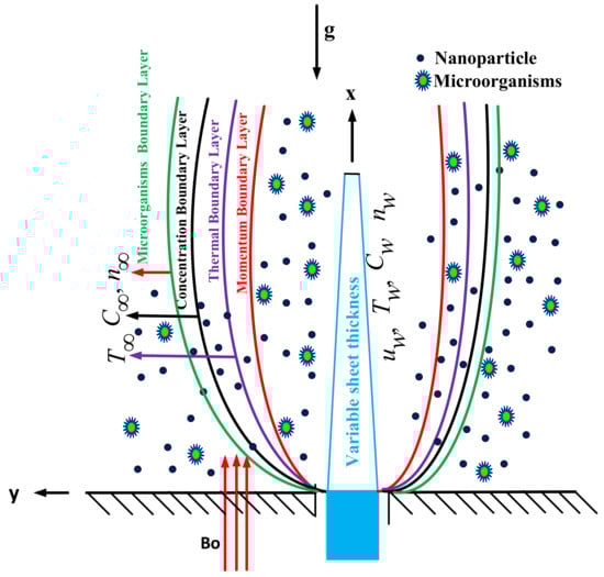
Figure 1.
The physical model of slender elastic sheets.
Here, ) includes velocity components in directions, respectively. Furthermore, the symbols in the above equations are defined in the nomenclature. The extra stress tensor of an Eyring–Powell model [58] is expressed as follows.
The governing equations can be written as follows [34,59,60].
Equation of continuity:
Equation of momentum:
Heat equation:
Nanoparticle concentration equation:
Concentration of microorganisms diffusion equation:
The boundary conditions of the present problem are as follows.
By assuming that thermophysical variables have a linear temperature dependence, we obtain the following.
The radiation under Rosseland approximations can be written as follows [61].
may be identified by extending in a Taylor series around while ignoring higher terms.
A mathematical technique that is suitable for some cases to convert partial differential equations into ordinary differential equation is called similarity transformation. This technique is sophisticated and is the most powerful and systematic for transforming PDEs into ODEs, and it is utilized widely in non-linear dynamical systems, especially in the field of computational fluid dynamics boundary value problems. To transform the above-mentioned governing equations into dimensionless forms, we introduce the following similarity variables, which guided us to avail non-dimensional forms of leading equations [59].
In the observation of above defined similarity variables, Equation (7) is identically satisfied, and Equations (8)–(11) can be written as follows:
which are subject to the boundary conditions in Equation (12):
where , , , , , and , , , , , , , and , .
We set the following possible changes for additional simplifications.
As a result, the nonlinear differential Equations (18)–(21) are changed to the following:
along with modified boundary constraints.
3. Physical Quantities
The influence of significant engineering parameters may be adequately investigated in this physical problem by calculating the localized magnitude of drag forces and the rate of thermal transports at the slender sheet. In terms of (skin friction), (Nusselt number), (Sherwood number), and (density of microorganisms), we have the following:
where , , , and are the shear stress, surface heat flux, surface mass flux, and the motile surface microorganism flux, respectively, which are defined as follows.
The following expressions are derived by utilizing Equations (11), (12) and (18).
4. Solution Procedure
The fundamental partial differential equations for the flow of MHD Eyring–Powell bioconvective nanofluids and the associated boundary conditions are transferred into a system of ordinary differential equations with similarity variables. The reduced Equations (24)–(27) and the associated boundary conditions (28) are then transformed into first-order differential equations and further transformed into initial value problems by labeling the variables as follows [62,63,64]. Accordingly, the above system of equations in matrix form can be expressed as follows:
and are subject to the initial conditions.
To solve the system of first-order ordinary differential Equation (38) with the help of the shooting method, nine initial conditions are required. Therefore, we estimate four unknown initial conditions The suitable estimations for four and s unknown missing conditions are chosen such that the four known boundary conditions are approximately satisfied for . Newton’s iterative scheme is applied to improve the accuracy of the missing initial conditions p, q, r and s until the desired approximation is met. The numerical computational has been performed for various physical emerging parameters for the appropriate computational domain [0, 10] instead of [0, ∞], where is fixed at 10 because there are no more variations in the results after . Newton’s iterative scheme is applied to improve the accuracy of the initial guesses until the desired approximation is obtained. The stopping criteria for the iterative process is .
5. Results and Discussion
This part aims to study the influence of parameters contained in the current problem on the momentum, temperature, and concentration of nanoparticles and microorganisms. To verify the exactness of the present computed outcomes with accessible distributed data, a comparison is completed between current computed outcomes and those in the available literature in a limiting case. Table 1 and Table 2 are displayed to authenticate the current numerical results of and with the previously published literature in Wakif [59] (skin friction) and [59,65] (Nusselt number), and these results achieved excellent agreements. We take the values of parameters as , and

Table 1.
Comparative of for different values of m by ignoring other parameters.
Table 2.
Comparing the current numerical findings for when and all others parameter are ignored.
The results of an investigation on Eyring–Powell nanofluid transportation caused by a stretched slender sheet of variable thickness are presented here. The fluctuation of skin friction factor was mentioned in Table 3. Because the physical nature of these parameters opposes the fluid stream, it, therefore, increases the resistance at the surface, increases parameters M, K, , , , and , and increased the magnitude of skin friction due to the accelerated flow. The skin fraction factor is reduced in a reciprocal manner by the thermal buoyancy parameter . The Nusselt number (local heat transfer rate) seems to increase immediately with the Prandtl number; however, it decreases reciprocally against excessive values of , , , and according to the contents of Table 4. Thermophoresis causes the Sherwood number to drop, whereas increased , , and caused it to increase (see Table 5).
Table 3.
Various numerical results for .
Table 4.
Various numerical results for .
Table 5.
Various numerical results for .
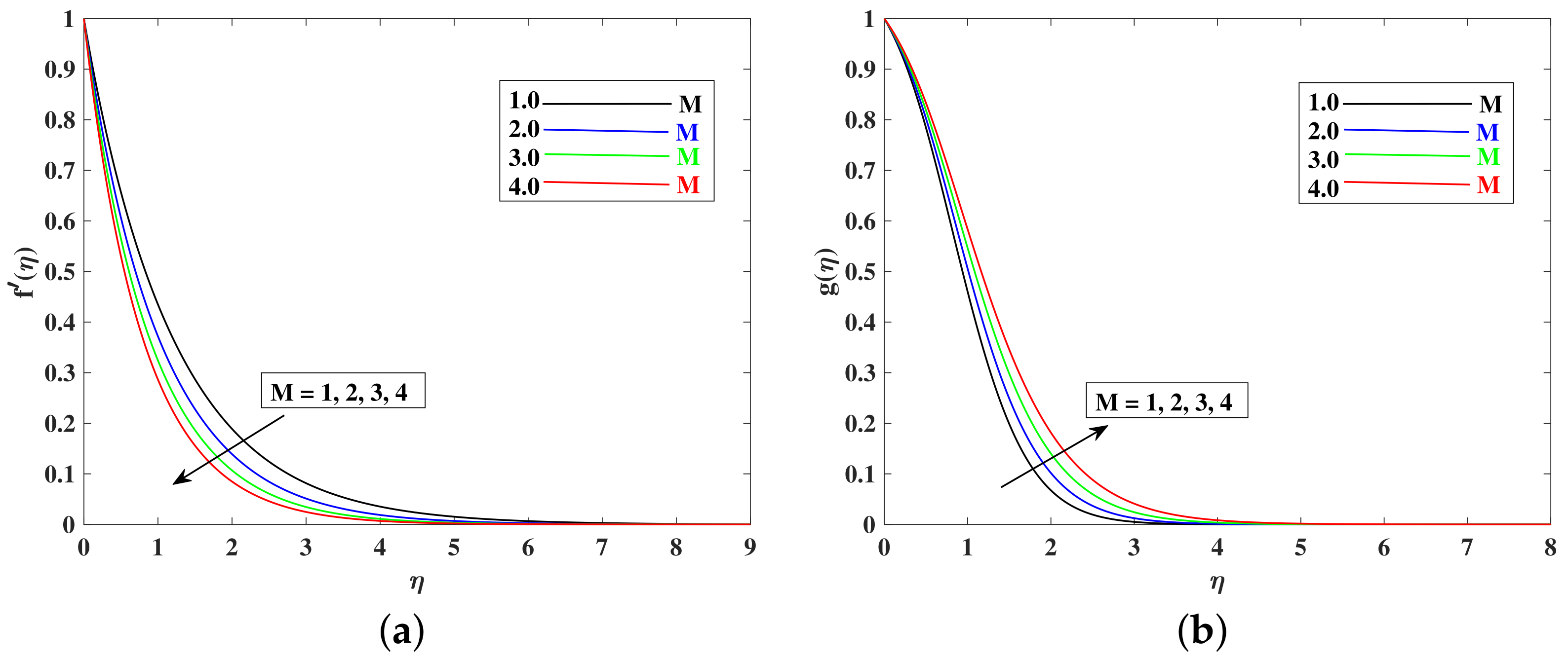
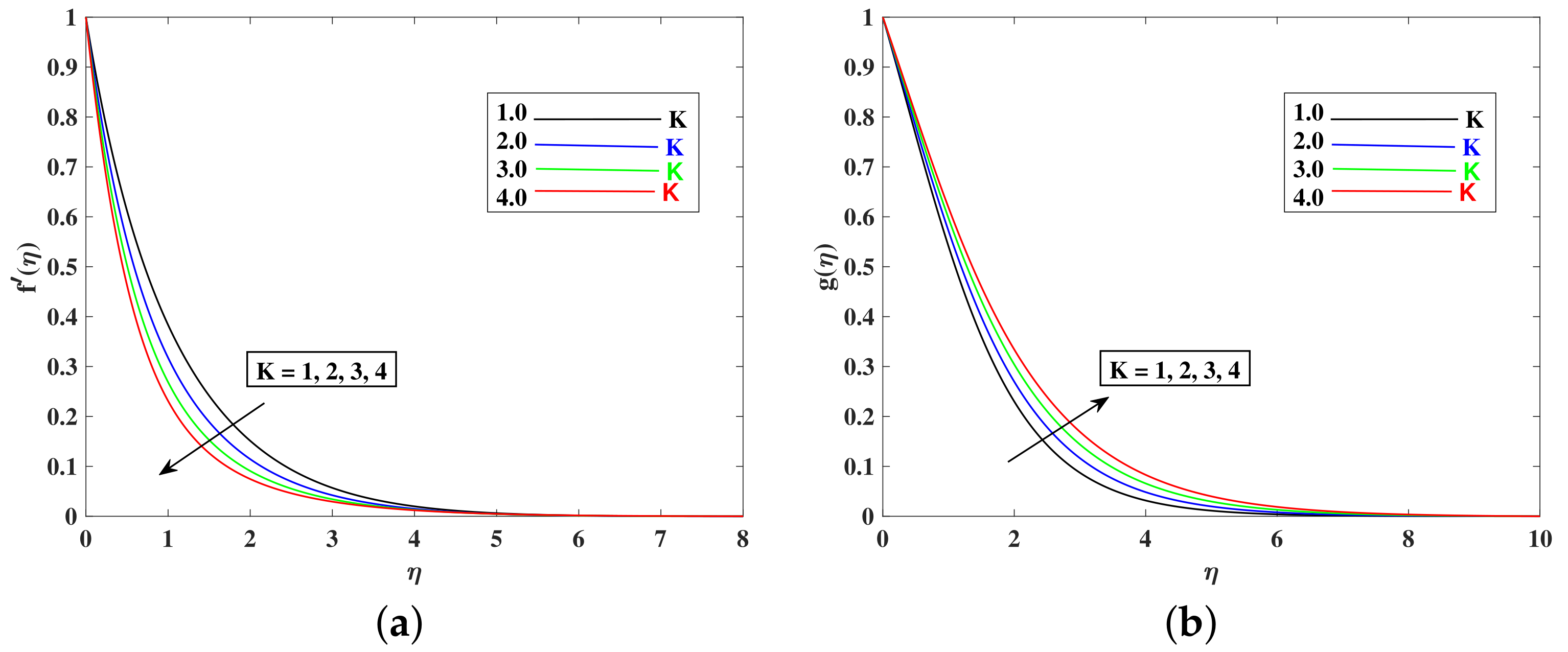
The impact of magnetic parameter M on momentum and temperature boundary layer is depicted in Figure 2a,b; in that order, growing values of M lower the curve of momentum but increase the curve of the thermal boundary layer, according to inspection. The increase in M is coupled with a stronger opposing force (Lorentz force) on the stream, resulting in a slowing of the speed and increase in temperature. Meanwhile, the fluid’s loss of kinetic energy is offset by a gain in heat energy, causing an increase in temperature. The effects of stronger porosity parameter K on and are scrutinized in Figure 3a,b, respectively. It is mentioned that K is inversely related to the permeability of the porous medium, which causes a decrement in momentum and increase in temperature. The sketches for momentum and thermal as influenced by thermal buoyancy parameter are shown in Figure 4a,b. Due to increasing buoyancy effects, the velocity increases directly with . The fluid’s heat energy is used to reduce the temperature throughout this procedure.
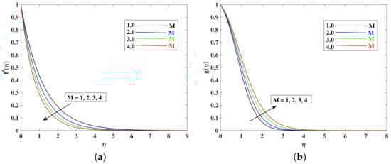
Figure 2.
Variation of M to influence the velocity and temperature profile. (a) Variation of M to influence the velocity. (b) Variation of M to influence the temperature.
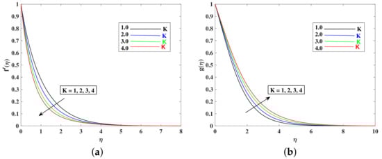
Figure 3.
Variation of K to influence the velocity and temperature profile. (a) Variation of K to influence the velocity. (b) Variation of K to influence the temperature.
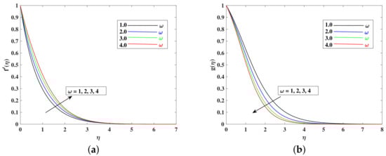
Figure 4.
Variation of to influence the velocity and temperature profile. (a) Variation of to influence the velocity. (b) Variation of to influence the temperature.
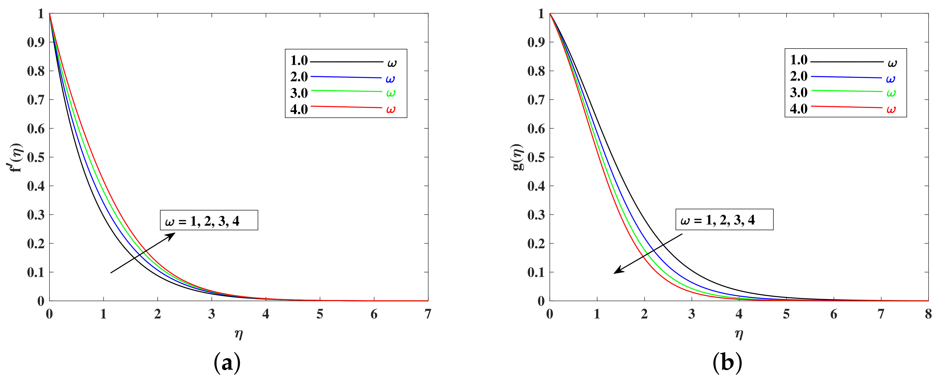
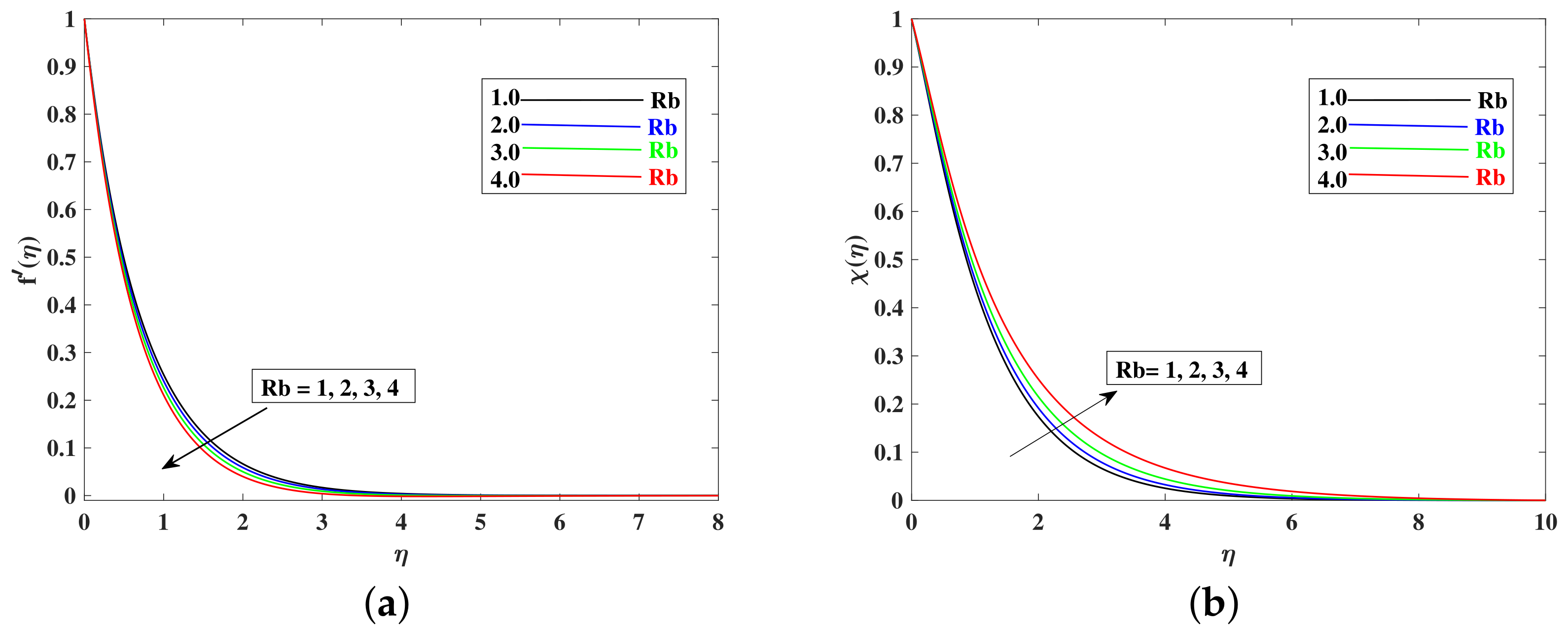
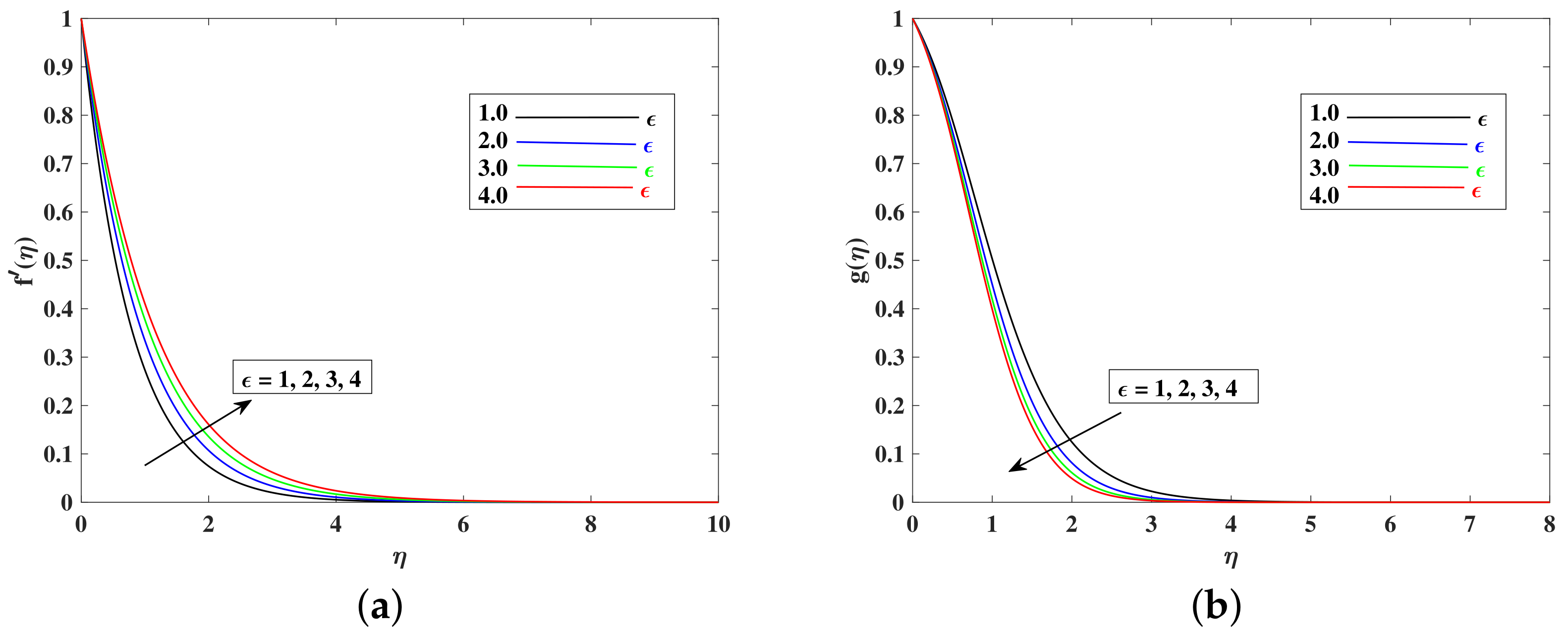
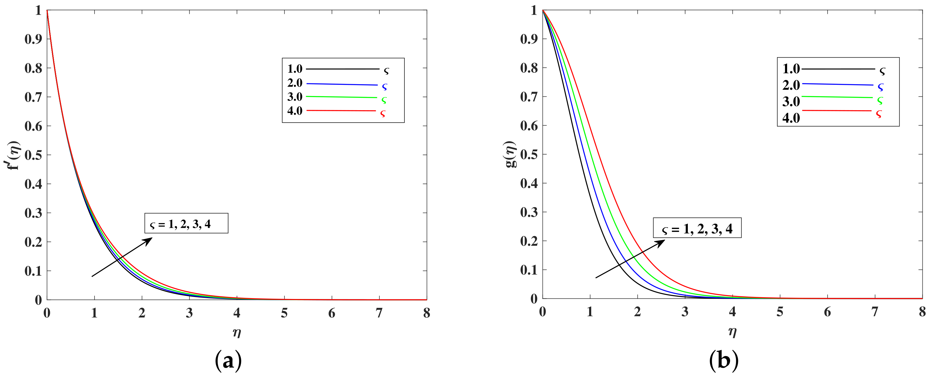
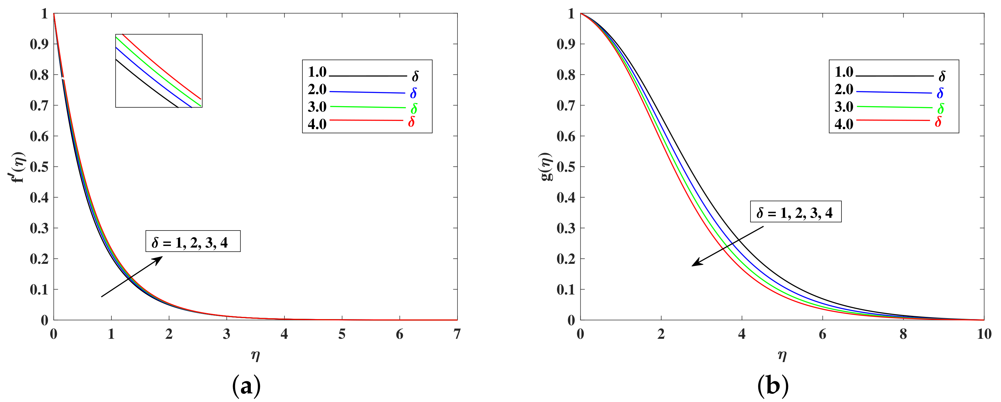
Figure 5a,b and Figure 6a,b portray the impacts of the buoyancy ratio parameter and Rayleigh number on the velocity and temperature profile. Both of these parameters decelerated the velocity profile and intensified the temperature. These parameters are inversely related to temperature differences: When temperature increases quicker, thermal buoyancy becomes less of a reason for velocity retardation. Figure 7a,b demonstrate the impact of fluid material parameters and on temperatures. The flow speed is quicker, and the thermal boundary is lower when parameter domains are boosted. This is because they are related inversely to viscosity. The boosted and mean lesser viscosity; hence, faster speeds result. When flow speed enhanced, the thermal profile is decremented. The impact of the wall thickness parameter on momentum and thermal boundary layer is observed in Figure 8a,b. Horizontal velocity increases as increases. When , and it declines with the increasing strength of , as stated by boundary condition . Then, should increase. With , the temperature of the fluid likewise increases, resulting in a greater blowing impact.
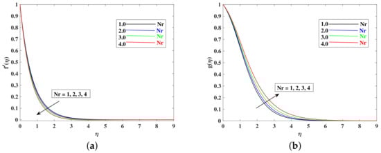
Figure 5.
Variation of to influence the velocity and temperature profile. (a) Variation of to influence the velocity. (b) Variation of to influence the temperature.
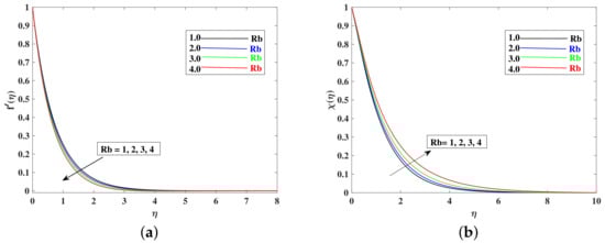
Figure 6.
Variation of to influence the velocity and bioconvection profile. (a) Variation of to influence the velocity. (b) Variation of to influence the bioconvection profile.
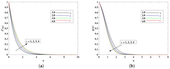
Figure 7.
Variation of to influence the velocity and temperature profile. (a) Variation of to influence the velocity. (b) Variation of to influence the temperature.
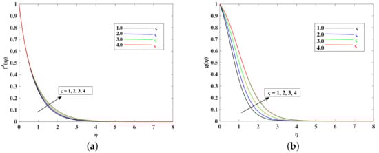
Figure 8.
Variation of to influence the velocity and temperature profile. (a) Variation of to influence the velocity. (b) Variation of to influence the temperature.
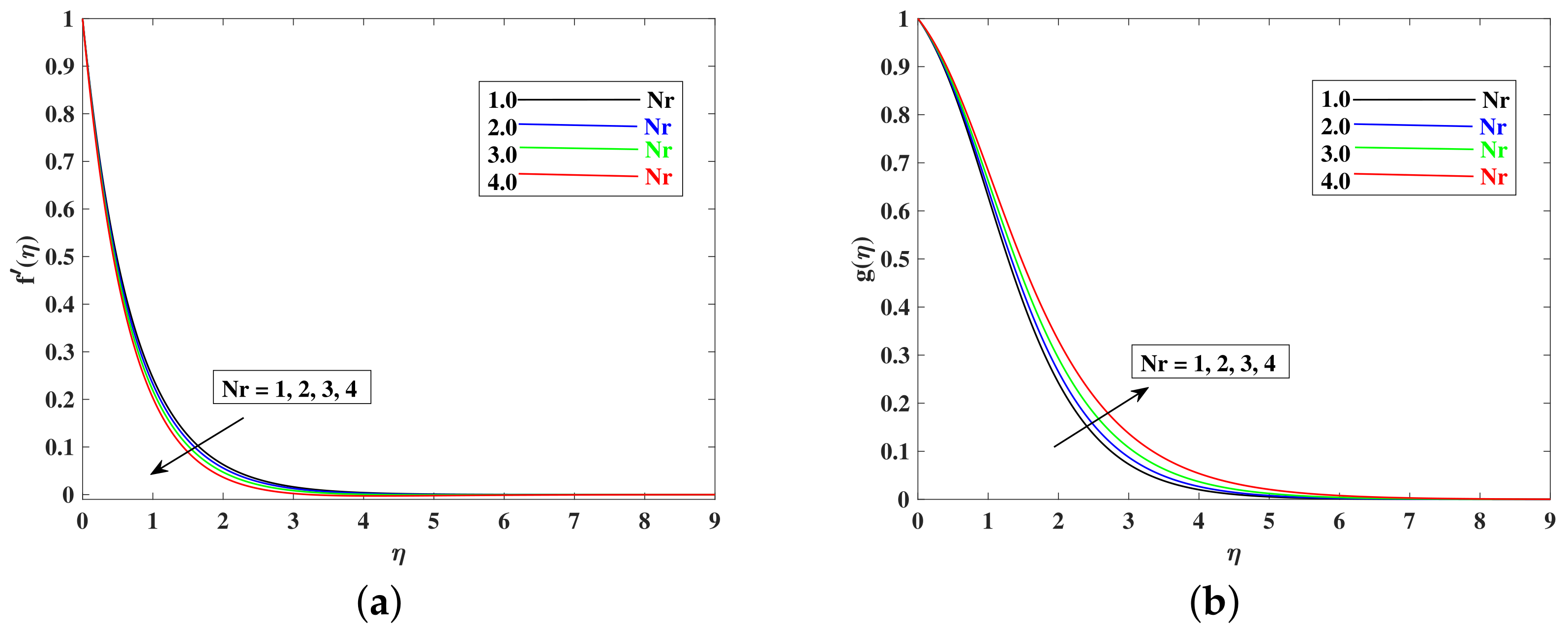
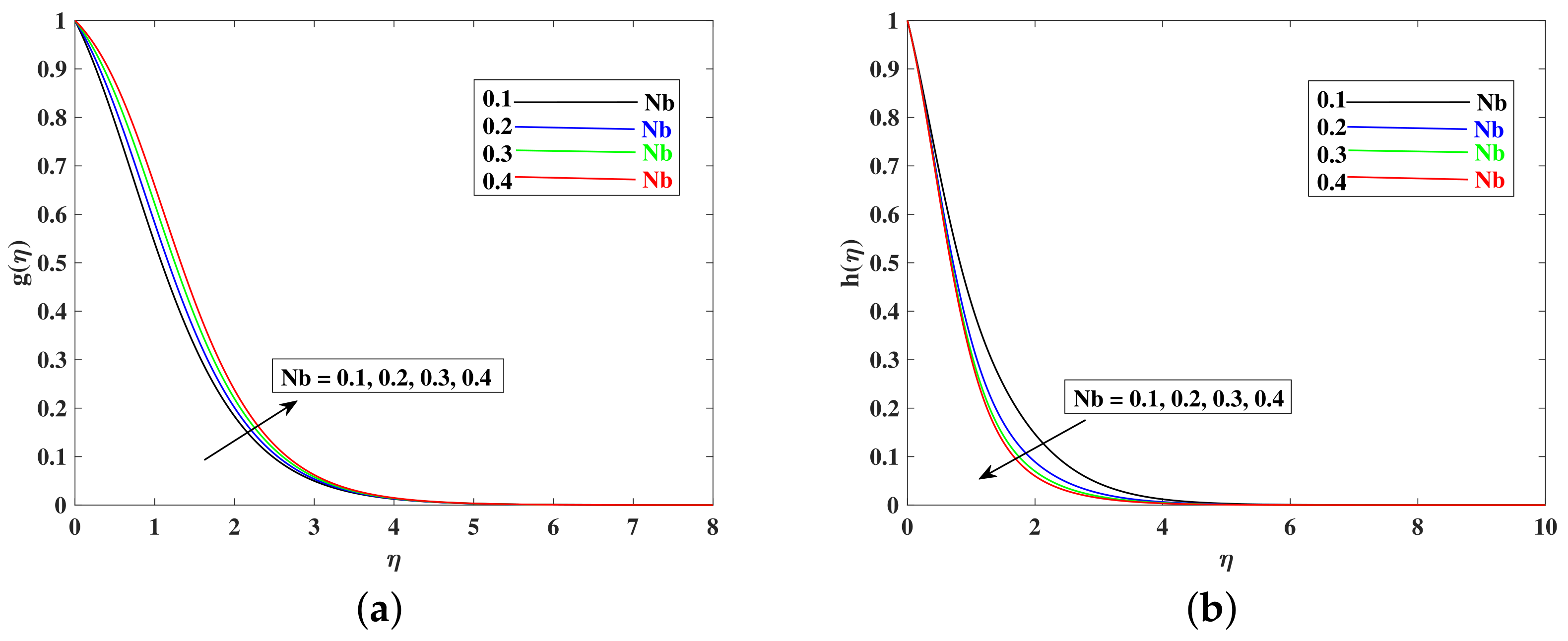
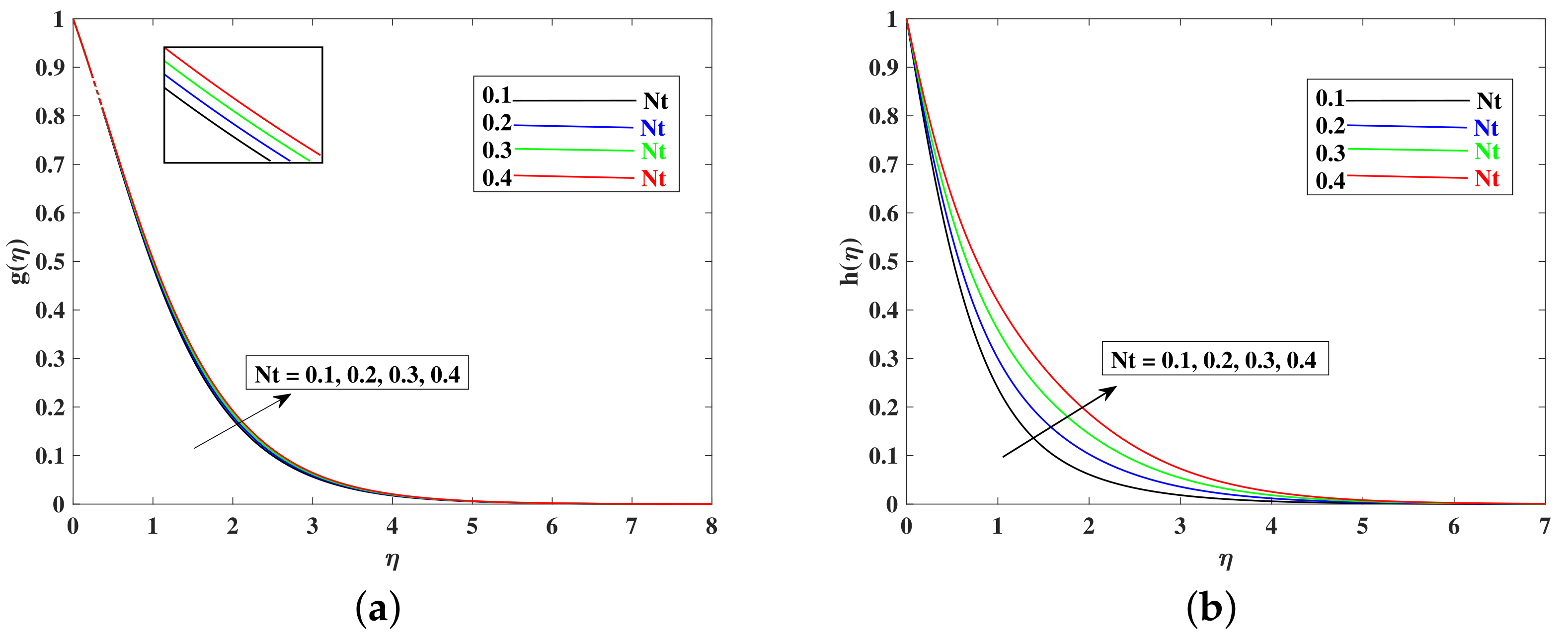
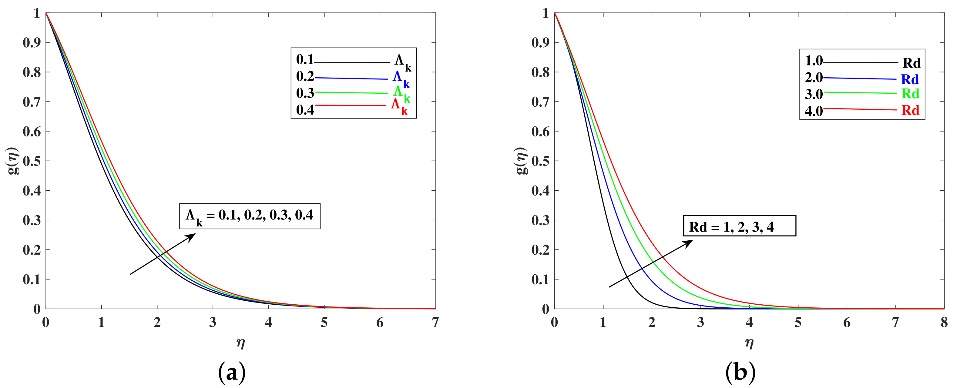
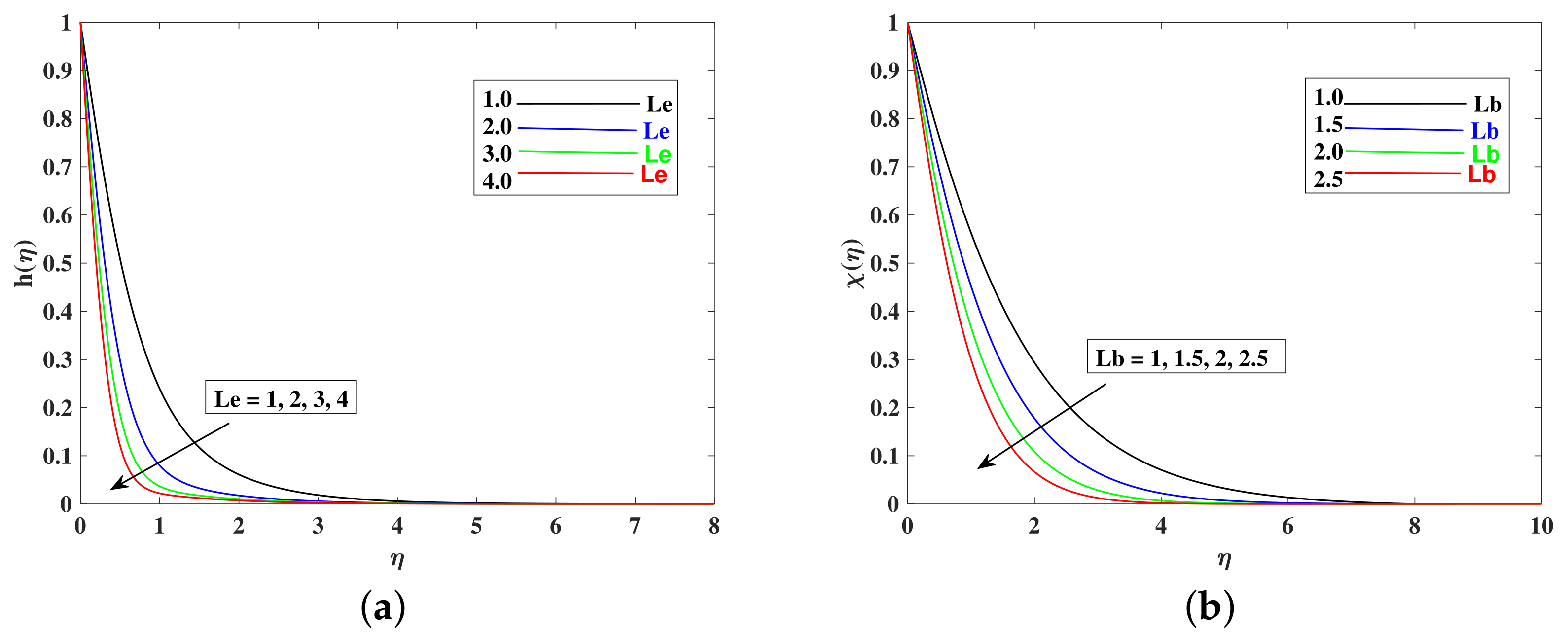
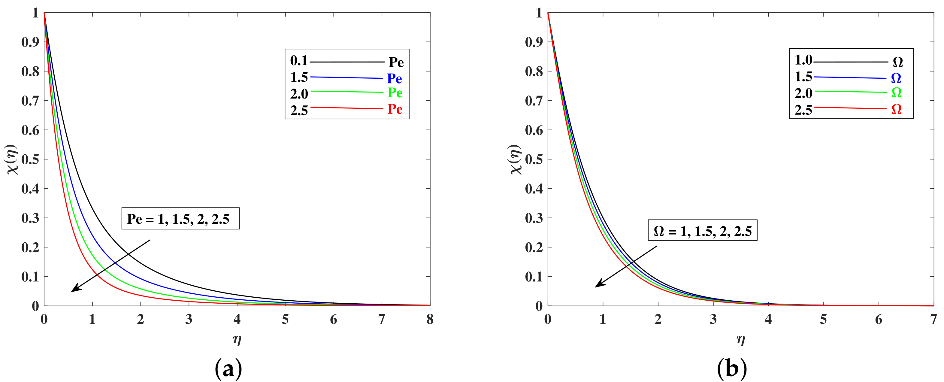
Figure 9a,b demonstrated the influence of material parameter on momentum profile . We observed from the figure that fluid velocities increase with higher . As it is directly in relation to the velocity of the surface and because of the greater stretching speed, the fluid’s velocity is also higher, and the temperature of the fluid decreases with an increase in . The fluctuation in temperatures and concentrations of nanoparticles is shown in Figure 10a,b to comprehend the influence of Brownian motion parameter . The higher the , the quicker the random movement of the nanoparticles, which results in increased heat diffusion and an increase in temperature. In addition, the rapid motion causes the concentration function to deteriorate. When particles transition from a heated to a cold state, a thermophoretic impact occurs. In Figure 11a,b, the impacts of the thermophoresis parameter on thermal and concentration boundary layer are displayed. The gradual migration of nanoparticles from hotter environments causes the temperature and concentration in the boundary layer area to increase. Figure 12a,b delineated the higher temperature of the fluid in direct response to (variable thermal conductivity parameter) and (Radiation parameter). The increments in include larger thermal conductivities; similarly, the higher inputs of mean larger radiation heat diffusion, which cause an increase in temperature. As the Lewis number is reciprocated with respect to mass diffusivity, its higher values cause a decline in concentration curve , as shown in Figure 13a. Similarly, against bioconvection Lewis number , the concentration profile of microorganisms is reduced (see Figure 13b) because is in an inverse relation to the diffusivity of microorganisms. Figure 14a,b with a rescaled microorganism distribution incorporates the nature of Peclet number and density ratio . When Peclet number and density ratio increases, the microorganism profile decreases.
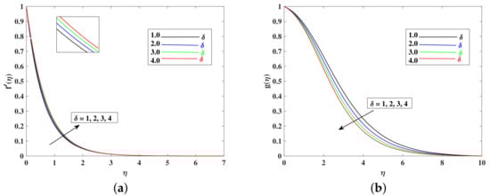
Figure 9.
Variation of to influence the velocity and temperature field. (a) Variation of to influence the velocity. (b) Variation of to influence the temperature.
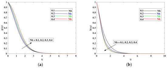
Figure 10.
Variation of to influence the temperature and concentration profile. (a) Variation of to influence the temperature. (b) Variation of to influence the concentration profile.
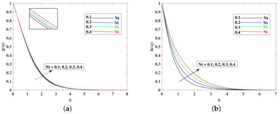
Figure 11.
Variation of to influence the temperature and concentration Profile. (a) Variation of to influence the temperature. (b) Variation of to influence the concentration profile.
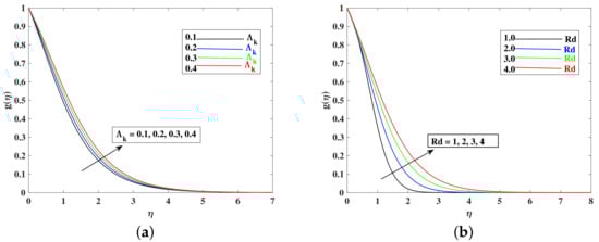
Figure 12.
Variation of and to influence the temperature profile. (a) Variation of to influence the temperature. (b) Variation of to influence the temperature.
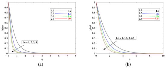
Figure 13.
Variation of and to influence the concentration and bioconvection profile. (a) Variation of to influence the concentration profile. (b) Variation of to influence the bioconvection profile.
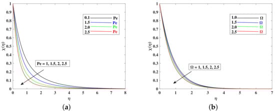
Figure 14.
Variation of (a) and (b) to influence the bioconvection field. (a) Variation of to influence the bioconvection profile. (b) Variation of to influence the bioconvection profile.
6. Conclusions
Boundary layer flows on MHD Eyring–Powell nanofluids across a slender elastic sheet of variable thicknesses are taken into account in this paper. The temperature and concentration constitutive equations are used to explore the Buongiorno model of nanofluids. Gyrotactic bioconvection features are also incorporated in flow phenomena. The results are obtained using the Runge–Kutta method approach in the MATLAB platform. The current research leads to the following delicate conclusions:
- The fluid’s velocity increases with larger values of the , , , and and it decrease with enhancements in M, K, , and because these parameters are responsible for decelerating the flow.
- The temperature profile enhanced with (Brownian motion), (Radiation parameter), and (thermophoretic parameter).
- Nanoparticle concentration increased when Nt is enhanced, and it decreased with the boosted inputs of , , and .
- The bioconvection profile decreased with higher inputs of parameters , , and .
- Skin friction increased with M, K, , , and . However, skin friction increased due to accelerated flows.
- The Nusselt number increased with higher values of , and it decreased when , , , and increased, because these parameters enhanced the temperature distribution relative to the reduced Nusselt number.
- To validate the findings, the current findings are compared to the previous literature.
By this computational endeavor, we successfully clarified the parametric effects on fluid dynamics. This study can be extended for Prandtl nanofluids, Carreau–Yasuda nanofluids, Maxewell nanofluids, viscoelastic Jeffrey’s nanofluids, and tangent hyperbolic nanofluids.
Author Contributions
Formal analysis, N.F.; Methodology, B.A.; Resources, M.I.; Software, S.U.R.; Supervision, J.D.C.; Validation, J.D.C.; Writing—original draft, A.M.; Writing—review & editing, N.A.S. All authors have read and agreed to the published version of the manuscript.
Funding
This research received no external funding.
Institutional Review Board Statement
Not Applicable.
Informed Consent Statement
Not Applicable.
Data Availability Statement
The numerical data used to support the findings of this study are included within the article.
Acknowledgments
This work was supported by the Technology Innovation Program (20018869, Development of Waste Heat and Waste Cold Recovery Bus Air-conditioning System to Reduce Heating and Cooling Load by ) funded By the Ministry of Trade, Industry & Energy (MOTIE, Korea).
Conflicts of Interest
The authors declare no conflict of interest.
Nomenclature
| Ambient motile microorganism | Dynanic viscosity | ||
| Concentration at surface | n | Density of motile microorganism | |
| Brownian diffusion coefficient | Radiative heat flux | ||
| Fluid velocity components along | Fluid velocity components along | ||
| g | Gravitational Acceleration | Heat flux | |
| T | Nanofluid temperature | Average volume of a microorganism | |
| Microorganisms density | Reynolds number | ||
| material liquid parameters of Powell-Eyring model | Electrical conductivity | ||
| Dimensionless velocity profile | Dimensionless nanofluid temperature | ||
| Dimensionless nanofluid concentration | Dimensionless density of motile microorganism | ||
| Mass density of nanoparticles | Thermophoretic diffusion coefficient | ||
| Density ratio of motile microorganisms | Temperature at surface | ||
| Variable viscosity | Kinematic viscosity | ||
| Mean absorption coeffiecient | Density of motile microorganism at surface | ||
| Uniform magnetic field | Ambient temperature | ||
| Fluid parameters | Ambient concentration | ||
| Variable thermal conductivity | Stefan-Boltzman constant | ||
| Specific heat | Linear temperature function | ||
| C | Nanoparticles concentration | Constant maximum cell swimming speed | |
| Variable viscosity | Thermal conductivity | ||
| M | Magnetic parameter | Thermal buoyancy parameter | |
| Thermophoresis parameter | Wall thickness parameter | ||
| Lewis number parameter | Prandtl number | ||
| Bioconvection Lewis number parameter | Peclet number | ||
| Buoyancy ratio parameter | Bioconvection Rayleigh number | ||
| Brownian motion | Radiation parameter | ||
| Mass flux | Motile microorganism flux | ||
| Skin friction coefficient | Nusselt number | ||
| Sherwood number | Density of motile microorganism |
References
- Choi, S.U.; Eastman, J.A. Enhancing Thermal Conductivity of Fluids with Nanoparticles; Technical Report; Argonne National Lab.: Lemont, IL, USA, 1995. [Google Scholar]
- Masuda, H.; Ebata, A.; Teramae, K. Alteration of thermal conductivity and viscosity of liquid by dispersing ultra-fine particles. Dispersion of Al2O3, SiO2 and TiO2 ultra-fine particles. Netsu Bussei 1993, 7, 227–233. [Google Scholar] [CrossRef]
- Buongiorno, J.; Hu, W. Nanofluid coolants for advanced nuclear power plants. In Proceedings of the ICAPP, Seoul, Korea, 15–19 May 2005; Volume 5, pp. 15–19. [Google Scholar]
- Buongiorno, J. Convective transport in nanofluids. J. Heat Transfer. Mar. 2006, 128, 240–250. [Google Scholar] [CrossRef]
- Kuznetsov, A.; Nield, D. Natural convective boundary-layer flow of a nanofluid past a vertical plate. Int. J. Therm. Sci. 2010, 49, 243–247. [Google Scholar] [CrossRef]
- Izadi, A.; Siavashi, M.; Rasam, H.; Xiong, Q. MHD enhanced nanofluid mediated heat transfer in porous metal for CPU cooling. Appl. Therm. Eng. 2020, 168, 114843. [Google Scholar] [CrossRef]
- Raza, J.; Mebarek-Oudina, F.; Ram, P.; Sharma, S. MHD flow of non-Newtonian molybdenum disulfide nanofluid in a converging/diverging channel with Rosseland radiation. Defect Diffus. Forum Trans. Tech. Publ. 2020, 401, 92–106. [Google Scholar] [CrossRef]
- Jamshed, W. Numerical investigation of MHD impact on Maxwell nanofluid. Int. Commun. Heat Mass Transf. 2021, 120, 104973. [Google Scholar] [CrossRef]
- Koriko, O.K.; Shah, N.A.; Saleem, S.; Chung, J.D.; Omowaye, A.J.; Oreyeni, T. Exploration of bioconvection flow of MHD thixotropic nanofluid past a vertical surface coexisting with both nanoparticles and gyrotactic microorganisms. Sci. Rep. 2021, 11, 16627. [Google Scholar] [CrossRef]
- Li, Y.X.; Alshbool, M.H.; Lv, Y.P.; Khan, I.; Khan, M.R.; Issakhov, A. Heat and mass transfer in MHD Williamson nanofluid flow over an exponentially porous stretching surface. Case Stud. Therm. Eng. 2021, 26, 100975. [Google Scholar] [CrossRef]
- Abbas, S.Z.; Khan, M.I.; Kadry, S.; Khan, W.A.; Israr-Ur-Rehman, M.; Waqas, M. Fully developed entropy optimized second order velocity slip MHD nanofluid flow with activation energy. Comput. Methods Programs Biomed. 2020, 190, 105362. [Google Scholar] [CrossRef]
- Dawar, A.; Shah, Z.; Kumam, P.; Alrabaiah, H.; Khan, W.; Islam, S.; Shaheen, N. Chemically reactive MHD micropolar nanofluid flow with velocity slips and variable heat source/sink. Sci. Rep. 2020, 10, 20926. [Google Scholar] [CrossRef]
- Shi, Q.H.; Hamid, A.; Khan, M.I.; Kumar, R.N.; Gowda, R.; Prasannakumara, B.; Shah, N.A.; Khan, S.U.; Chung, J.D. Numerical study of bio-convection flow of magneto-cross nanofluid containing gyrotactic microorganisms with activation energy. Sci. Rep. 2021, 11, 16030. [Google Scholar] [CrossRef] [PubMed]
- Ashraf, M.Z.; Rehman, S.U.; Farid, S.; Hussein, A.K.; Ali, B.; Shah, N.A.; Weera, W. Insight into Significance of Bioconvection on MHD Tangent Hyperbolic Nanofluid Flow of Irregular Thickness across a Slender Elastic Surface. Mathematics 2022, 10, 2592. [Google Scholar] [CrossRef]
- Ali, L.; Ali, B.; Liu, X.; Iqbal, T.; Zulqarnain, R.M.; Javid, M. A comparative study of unsteady MHD Falkner-Skan wedge flow for non-Newtonian nanofluids considering thermal radiation and activation energy. Chin. J. Phys. 2022, 77, 1625–1638. [Google Scholar] [CrossRef]
- Habib, D.; Salamat, N.; Abdal, S.H.S.; Ali, B. Numerical investigation for MHD Prandtl nanofluid transportation due to a moving wedge: Keller box approach. Int. Commun. Heat Mass Transf. 2022, 135, 106141. [Google Scholar] [CrossRef]
- Wang, J.; Mustafa, Z.; Siddique, I.; Ajmal, M.; Jaradat, M.M.; Rehman, S.U.; Ali, B.; Ali, H.M. Computational Analysis for Bioconvection of Microorganisms in Prandtl Nanofluid Darcy–Forchheimer Flow across an Inclined Sheet. Nanomaterials 2022, 12, 1791. [Google Scholar] [CrossRef]
- Younis, O.; Alizadeh, M.; Kadhim Hussein, A.; Ali, B.; Biswal, U.; Hasani Malekshah, E. MHD Natural Convection and Radiation over a Flame in a Partially Heated Semicircular Cavity Filled with a Nanofluid. Mathematics 2022, 10, 1347. [Google Scholar] [CrossRef]
- Ali, L.; Ali, B.; Liu, X.; Ahmed, S.; Shah, M.A. Analysis of bio-convective MHD Blasius and Sakiadis flow with Cattaneo-Christov heat flux model and chemical reaction. Chin. J. Phys. 2021, 77, 1963–1975. [Google Scholar] [CrossRef]
- Gupta, R.; Sridhar, T. Viscoelastic effects in non-Newtonian flows through porous media. Rheol. Acta 1985, 24, 148–151. [Google Scholar] [CrossRef]
- Subhas, A.; Veena, P. Visco-elastic fluid flow and heat transfer in a porous medium over a stretching sheet. Int. J. Non-Linear Mech. 1998, 33, 531–540. [Google Scholar] [CrossRef]
- Prasad, K.; Abel, M.S.; Khan, S.K. Momentum and heat transfer in visco-elastic fluid flow in a porous medium over a non-isothermal stretching sheet. Int. J. Numer. Methods Heat Fluid Flow 2000, 10, 786–801. [Google Scholar] [CrossRef]
- Seddeek, M.; Salama, F.A. The effects of temperature dependent viscosity and thermal conductivity on unsteady MHD convective heat transfer past a semi-infinite vertical porous moving plate with variable suction. Comput. Mater. Sci. 2007, 40, 186–192. [Google Scholar] [CrossRef]
- Zheng, L.; Zhang, C.; Zhang, X.; Zhang, J. Flow and radiation heat transfer of a nanofluid over a stretching sheet with velocity slip and temperature jump in porous medium. J. Frankl. Inst. 2013, 350, 990–1007. [Google Scholar] [CrossRef]
- Dessie, H.; Kishan, N. MHD effects on heat transfer over stretching sheet embedded in porous medium with variable viscosity, viscous dissipation and heat source/sink. Ain Shams Eng. J. 2014, 5, 967–977. [Google Scholar] [CrossRef]
- Mahabaleshwar, U.; Anusha, T.; Hatami, M. The MHD Newtonian hybrid nanofluid flow and mass transfer analysis due to super-linear stretching sheet embedded in porous medium. Sci. Rep. 2021, 11, 22518. [Google Scholar] [CrossRef]
- Vishalakshi, A.; Mahabaleshwar, U.; Sheikhnejad, Y. Impact of MHD and Mass Transpiration on Rivlin–Ericksen Liquid Flow over a Stretching Sheet in a Porous Media with Thermal Communication. Transp. Porous Media 2022, 142, 353–381. [Google Scholar] [CrossRef]
- Kothandapani, M.; Srinivas, S. Peristaltic transport of a Jeffrey fluid under the effect of magnetic field in an asymmetric channel. Int. J. Non-Linear Mech. 2008, 43, 915–924. [Google Scholar] [CrossRef]
- Mekheimer, K.S. Effect of the induced magnetic field on peristaltic flow of a couple stress fluid. Phys. Lett. A 2008, 372, 4271–4278. [Google Scholar] [CrossRef]
- Nadeem, S.; Akbar, N.S. Influence of heat transfer on a peristaltic flow of Johnson Segalman fluid in a non uniform tube. Int. Commun. Heat Mass Transf. 2009, 36, 1050–1059. [Google Scholar] [CrossRef]
- Mekheimer, K.S. Peristaltic flow of a couple stress fluid in an annulus: Application of an endoscope. Phys. A Stat. Mech. Its Appl. 2008, 387, 2403–2415. [Google Scholar] [CrossRef]
- Hayat, T.; Momoniat, E.; Mahomed, F.M. Peristaltic MHD flow of third grade fluid with an endoscope and variable viscosity. J. Nonlinear Math. Phys. 2008, 15, 91–104. [Google Scholar] [CrossRef]
- Srinivas, S.; Gayathri, R.; Kothandapani, M. The influence of slip conditions, wall properties and heat transfer on MHD peristaltic transport. Comput. Phys. Commun. 2009, 180, 2115–2122. [Google Scholar] [CrossRef]
- Bilal, M.; Ashbar, S. Flow and heat transfer analysis of Eyring-Powell fluid over stratified sheet with mixed convection. J. Egypt. Math. Soc. 2020, 28, 40. [Google Scholar] [CrossRef]
- Akbar, N.S.; Ebaid, A.; Khan, Z. Numerical analysis of magnetic field effects on Eyring-Powell fluid flow towards a stretching sheet. J. Magn. Magn. Mater. 2015, 382, 355–358. [Google Scholar] [CrossRef]
- Ibrahim, W.; Anbessa, T. Hall and Ion slip effects on mixed convection flow of Eyring-Powell nanofluid over a stretching surface. Adv. Math. Phys. 2020, 2020. [Google Scholar] [CrossRef]
- Javed, T.; Ali, N.; Abbas, Z.; Sajid, M. Flow of an Eyring-Powell non-Newtonian fluid over a stretching sheet. Chem. Eng. Commun. 2013, 200, 327–336. [Google Scholar] [CrossRef]
- Vishalakshi, A.; Mahabaleshwar, U.; Sarris, I.E. An MHD Fluid Flow over a Porous Stretching/Shrinking Sheet with Slips and Mass Transpiration. Micromachines 2022, 13, 116. [Google Scholar] [CrossRef] [PubMed]
- Saravana, R.; Hemadri Reddy, R.; Narasimha Murthy, K.; Makinde, O. Thermal radiation and diffusion effects in MHD Williamson and Casson fluid flows past a slendering stretching surface. Heat Transfer 2022, 51, 3187–3200. [Google Scholar] [CrossRef]
- Sarada, K.; Gowda, R.J.P.; Sarris, I.E.; Kumar, R.N.; Prasannakumara, B.C. Effect of magnetohydrodynamics on heat transfer behaviour of a non-Newtonian fluid flow over a stretching sheet under local thermal non-equilibrium condition. Fluids 2021, 6, 264. [Google Scholar] [CrossRef]
- Ajeeb, W.; Oliveira, M.S.; Martins, N.; Murshed, S.S. Forced convection heat transfer of non-Newtonian MWCNTs nanofluids in microchannels under laminar flow. Int. Commun. Heat Mass Transf. 2021, 127, 105495. [Google Scholar] [CrossRef]
- Raptis, A.; Perdikis, C.; Takhar, H.S. Effect of thermal radiation on MHD flow. Appl. Math. Comput. 2004, 153, 645–649. [Google Scholar] [CrossRef]
- Hayat, T.; Abbas, Z.; Sajid, M.; Asghar, S. The influence of thermal radiation on MHD flow of a second grade fluid. Int. J. Heat Mass Transf. 2007, 50, 931–941. [Google Scholar] [CrossRef]
- Cortell, R. Effects of viscous dissipation and radiation on the thermal boundary layer over a nonlinearly stretching sheet. Phys. Lett. A 2008, 372, 631–636. [Google Scholar] [CrossRef]
- Rashidi, M.; Ganesh, N.V.; Hakeem, A.A.; Ganga, B. Buoyancy effect on MHD flow of nanofluid over a stretching sheet in the presence of thermal radiation. J. Mol. Liq. 2014, 198, 234–238. [Google Scholar] [CrossRef]
- Ali, L.; Ali, B.; Ghori, M.B. Melting effect on Cattaneo–Christov and thermal radiation features for aligned MHD nanofluid flow comprising microorganisms to leading edge: FEM approach. Comput. Math. Appl. 2022, 109, 260–269. [Google Scholar] [CrossRef]
- Sudarsana Reddy, P.; Sreedevi, P. Impact of chemical reaction and double stratification on heat and mass transfer characteristics of nanofluid flow over porous stretching sheet with thermal radiation. Int. J. Ambient Energy 2022, 43, 1626–1636. [Google Scholar] [CrossRef]
- Childress, S.; Levandowsky, M.; Spiegel, E. Pattern formation in a suspension of swimming microorganisms: Equations and stability theory. J. Fluid Mech. 1975, 69, 591–613. [Google Scholar] [CrossRef]
- Hill, N.; Pedley, T.; Kessler, J.O. Growth of bioconvection patterns in a suspension of gyrotactic in a layer of finite depth. J. Fluid Mech. 1989, 208, 509–543. [Google Scholar] [CrossRef]
- Khan, W.; Makinde, O. MHD nanofluid bioconvection due to gyrotactic microorganisms over a convectively heat stretching sheet. Int. J. Therm. Sci. 2014, 81, 118–124. [Google Scholar] [CrossRef]
- Alqarni, M.; Waqas, H.; Imran, M.; Alghamdi, M.; Muhammad, T. Thermal transport of bio-convection flow of micropolar nanofluid with motile microorganisms and velocity slip effects. Phys. Scr. 2020, 96, 015220. [Google Scholar] [CrossRef]
- Zadeh, S.M.H.; Mehryan, S.; Sheremet, M.A.; Izadi, M.; Ghodrat, M. Numerical study of mixed bio-convection associated with a micropolar fluid. Therm. Sci. Eng. Prog. 2020, 18, 100539. [Google Scholar]
- Chu, Y.M.; Khan, M.I.; Khan, N.B.; Kadry, S.; Khan, S.U.; Tlili, I.; Nayak, M. Significance of activation energy, bio-convection and magnetohydrodynamic in flow of third grade fluid (non-Newtonian) towards stretched surface: A Buongiorno model analysis. Int. Commun. Heat Mass Transf. 2020, 118, 104893. [Google Scholar] [CrossRef]
- Alshomrani, A.S. Numerical investigation for bio-convection flow of viscoelastic nanofluid with magnetic dipole and motile microorganisms. Arab. J. Sci. Eng. 2021, 46, 5945–5956. [Google Scholar] [CrossRef]
- Asjad, M.I.; Ur Rehman, S.; Ahmadian, A.; Salahshour, S.; Salimi, M. First Solution of Fractional Bioconvection with Power Law Kernel for a Vertical Surface. Mathematics 2021, 9, 1366. [Google Scholar] [CrossRef]
- Jawad, M.; Saeed, A.; Khan, A.; Islam, S. MHD bioconvection Darcy-Forchheimer flow of Casson nanofluid over a rotating disk with entropy optimization. Heat Transf. 2021, 50, 2168–2196. [Google Scholar] [CrossRef]
- Khan, M.; Salahuddin, T.; Malik, M.; Alqarni, M.; Alqahtani, A. Numerical modeling and analysis of bioconvection on MHD flow due to an upper paraboloid surface of revolution. Phys. A Stat. Mech. Its Appl. 2020, 553, 124231. [Google Scholar] [CrossRef]
- Ara, A.; Khan, N.A.; Khan, H.; Sultan, F. Radiation effect on boundary layer flow of an Eyring–Powell fluid over an exponentially shrinking sheet. Ain Shams Eng. J. 2014, 5, 1337–1342. [Google Scholar] [CrossRef]
- Wakif, A. A novel numerical procedure for simulating steady MHD convective flows of radiative Casson fluids over a horizontal stretching sheet with irregular geometry under the combined influence of temperature-dependent viscosity and thermal conductivity. Math. Probl. Eng. 2020, 2020. [Google Scholar] [CrossRef]
- Hayat, T.; Ullah, I.; Alsaedi, A.; Farooq, M. MHD flow of Powell-Eyring nanofluid over a non-linear stretching sheet with variable thickness. Results Phys. 2017, 7, 189–196. [Google Scholar] [CrossRef]
- Rosseland, S. Astrophysik: Auf Atomtheoretischer Grundlage; Springer: Berlin/Heidelberg, Germany, 2013; Volume 11. [Google Scholar]
- Rehman, S.U.; Mariam, A.; Ullah, A.; Asjad, M.I.; Bajuri, M.Y.; Pansera, B.A.; Ahmadian, A. Numerical computation of buoyancy and radiation effects on MHD micropolar nanofluid flow over a stretching/shrinking sheet with heat source. Case Stud. Therm. Eng. 2021, 25, 100867. [Google Scholar] [CrossRef]
- Wang, F.; Asjad, M.I.; Ur Rehman, S.; Ali, B.; Hussain, S.; Gia, T.N.; Muhammad, T. MHD Williamson Nanofluid Flow over a Slender Elastic Sheet of Irregular Thickness in the Presence of Bioconvection. Nanomaterials 2021, 11, 2297. [Google Scholar] [CrossRef]
- Wei, Y.; Rehman, S.U.; Fatima, N.; Ali, B.; Ali, L.; Chung, J.D.; Shah, N.A. Significance of Dust Particles, Nanoparticles Radius, Coriolis and Lorentz Forces: The Case of Maxwell Dusty Fluid. Nanomaterials 2022, 12, 1512. [Google Scholar] [CrossRef] [PubMed]
- Wang, C. Free convection on a vertical stretching surface. ZAMM-J. Appl. Math. Mech./Z. Angew. Math. Mech. 1989, 69, 418–420. [Google Scholar] [CrossRef]

Publisher’s Note: MDPI stays neutral with regard to jurisdictional claims in published maps and institutional affiliations. |
© 2022 by the authors. Licensee MDPI, Basel, Switzerland. This article is an open access article distributed under the terms and conditions of the Creative Commons Attribution (CC BY) license (https://creativecommons.org/licenses/by/4.0/).