Infinite-Server Resource Queueing Systems with Different Types of Markov-Modulated Poisson Process and Renewal Arrivals

Abstract

In this paper, we propose models that significantly expand the scope of practical applications, namely, queueing systems with various nodes for processing heterogeneous data that require arbitrary resource capacities for their service. When a customer arrives in the system, the customer typeis randomly selected according to a set of probabilities. Then the customer goes to the server of the corresponding device type, where its service is performed during a random time period with a distribution function depending on the type of customer. Moreover, each customer requires a random amount of resources, of which the distribution function also depends on the customer type, but is independent of its service time. The aim of this research was to develop a heterogeneous queueing resource system with an unlimited number of servers and an arrival process in the form of a Markov-modulated Poisson process or stationary renewal process, and with requests for a random number of heterogeneous resources. We have performed analysis under conditions of growing intensity of the arrival process. Here we formulate the theorems and prove that under high-load conditions, the joint asymptotic probability distribution of the n-dimensional process of the total amounts of the occupied resources in the system is a multidimensional Gaussian distribution with parameters that are dependent on the type of arrival process. As a result of numerical and simulation experiments, conclusions are drawn on the limits of the applicability of the obtained asymptotic results. The dependence of the convergence of experimental results on the type of distribution of the system parameters (including the distributions of the service time and of the customer capacity) are also studied. The results of the approximations may be applied to estimating the optimal total number of resources for a system with a limited amount of resources.

1. Introduction

The development of modern info-communication systems and networks has provided access to many different services for use by subscribers. In modern conditions, users are not only people; rather, a variety of devices can also be connected to the network. At the same time, the rapid growth of the generated load can cause overloads in some parts of the network, which lead to the deterioration of quality. There are more and more opportunities for the users’ behavior to influence the formation of incoming streams, the frequency of calls, the length of messages, their number, etc. Many multimedia and service applications on subscriber devices can automatically generate such requests without any restrictions. Overflows begin to appear on sections of the network, which leads to the failure of network segments, leading to the complete failure of its operation. Identifying and investigating the effect of aspects of behavior on the quality of the network allows one to plan and prepare a network in advance in such a way as to reduce the loss of calls. The greatest area of interest, from a practical perspective, is the consideration of extreme working conditions, for example, overload conditions, when the state of the network differs from the normal (planned) state.

The theoretical and the applied foundations of research in the field of data transmission and processing in info-communication systems are based mainly on probability theory, random process theory, queueing theory, and teletraffic theory. The initial research in the field of computer networks, presented in the works of L. Kleinrock, G. P. Basharin, M. Schwartz, and V. M. Vishnevsky, as well as in the works of A. K. Erlang, was based on simplified models of information systems with the Poisson arrival process and an exponential distribution of the packets’ service times. The monographs of the Russian and foreign scientists G. P. Basharin, V. M. Vishnevsky, A. N. Dudin, A. Melikov, K. E. Samouylov, E. Gelenbe, W. Whitt, G. Pujolle, D. Gross, C. Harris, L. Kleinrock, J. W. Roberts, and M. Schneps-Schneppe give a detailed overview of modern applications of the queueing models in the field of telecommunications, modern computer networks, and information systems [1,2,3,4].

The analysis of modern communication systems is complicated by the fact that requests for data transfers are not homogeneous. The servicing of such applications may differ both in terms of the time of service and the volume of additional resources provided. To reduce data transmission losses, it is necessary to take into account the random amount of requested resources and service characteristics. Identifying these aspects and analyzing their impact on systems allows networks to be optimized to reduce losses.

In classical queueing system (QSs), the devices and waiting places (buffer, orbit) play the role of discrete resources which are necessary for maintenance. In real-world systems, in addition to the devices and the wait locations, customers may require various resources (both discrete and continuous) to be occupied while waiting for a service to start, or during a service, or while the requirement is in the system. In this case, the terms “resource QS” or “QS with a random volume of requirements” are used. The random volume of the resource occupied by the customer for the entire duration of their stay in the system can be either discrete or continuous. Resources are related to the most commonly used amount of memory. At the same time, in wireless networks, such as long-term evolution (4G LTE) networks or New Radio (5G NR), network bandwidth is understood as a resource, which is notoriously limited and must be distributed when the user receives a call and released at the end of the session by the device or a separate system. E. L. Romm and V. V. Skitovich first formulated a generalization of the Erlang problem, in which each arriving customer has some information quality, which the authors call the amount of the requirement [5]. Later, O. Tikhonenko, M. Kawecka, W. M. Kempa, E. Morozov, K. E. Samouylov made a significant contribution to the development of research methods on resource QSs [6,7,8,9,10,11,12].

In their works, the authors considered a QS with a random volume of requirements, as a class of systems with some capacity, which is dependent upon or independent of the volume of requirements and the time of service. Resource QSs with limited resources have been used in some works as models of the next generation of wireless communication networks [13,14,15].

Despite the large list of applied problems that can be solved using queuing models with an arrival process involving a random amount of requirements, to date, accurate analytical results regarding the study of the total volume of requirements in the system exist only for the case of the Poisson arrival process and classical QSs. However, the results of studies of real flows indicate the presence of a correlation and a large variance between the moments of receipt of requests, which has led to the use of models of correlated flows. Therefore, the queueing theory with correlated flows developed by G. P. Basharin, M. Neuts, D. Lucantoni [16,17] has found wide application in the study of telecommunication systems.

However, it should be noted that for resource systems with non-Poisson arrival processes (non-Markov systems), there is currently no universal approach to the study and most of the results are obtained by means of simulations, and analytical results have been obtained only for some special cases. Therefore, in this article we propose to use asymptotic methods for the study of a QS developed at the Tomsk scientific school of applied probabilistic analysis under the guidance of A. A. Nazarov [18]. Such methods make it possible to obtain asymptotic expressions acceptable for practice regarding the desired characteristics of the system in cases where their analytical analysis is impossible.

The first results for a QS with an infinite number of servers were obtained in the middle of the last century in [19,20,21,22]. The main distinguishing feature of systems with an unlimited number of servers is the lack of queues and the dropping of service applications. Markovian QSs with an unlimited number of servicing devices were investigated in the first half of the 20th century, when the most of the problems of queueing theory were solved for models with the stationary Poisson arrival process and an exponential time for servicing applications. It was shown that the number of occupied devices in the M/M/∞ system is distributed according to Poisson’s law. For systems with an arbitrary function of the distribution of the service time, B. A. Sevostyanov solved the Erlang problem for M/G/N systems in 1958 and showed that as $N\to \infty$ the distribution converges to the Poisson distribution. A similar result was obtained in 1969 by L. Takacs [23], who showed that in stationary mode, the number of customers in the M/G/∞ system has a Poisson distribution, which depends on the average speed of receipt of applications and the average time of call service.

In the work of D. Eaglehart [24], a diffusion approximation of the number of occupied devices for the M/M/∞ model with identical independent servers was obtained under the condition of a high incoming flow intensity ($\lambda \to \infty$) and fixed service time characteristics $\mu$, and it was shown that in stationary mode, it is distributed according to the normal law with parameter $\frac{\lambda }{\mu }$. Similar results were first obtained for non-exponential service time by A. A. Borovkov, and later in the papers of other scientists [25,26,27].

As a rule, when studying multi-server systems, it is usually assumed that the servers are identical and that arriving requests can occupy an arbitrary server to be serviced. QSs with heterogeneous servers are much less frequently studied, which makes them a more interesting object of research [28,29,30,31,32,33,34]. Nontrivial optimization problems often arise related to the assignment of servers to arriving orders depending on the ratio of the service rates of the facilities and the costs of their use.

Non-trivial optimization problems also often arise related to the assignment of servers to incoming calls depending on the ratio of the service rates of the funds and the costs of their use. For example, in the theory of teletraffic, the concepts of “fast” and “slow” communication channels are used. In this case, a situation is possible when a copy is created for the incoming request, which is transmitted via another communication channel. In this case, as a mathematical model, one can use a QS with parallel service [35].

In this paper, we propose models that significantly expand the scope of practical applications, namely, a QS with various nodes for processing heterogeneous data (information) that require arbitrary resource capacities for their service. When a customer arrives in the system, its customer type is randomly selected according to the set of probabilities $p_i$. Then the customer goes to a server of the corresponding device type, where its service is performed during a random time interval with a distribution function depending on the type of customer. Moreover, each customer requires a random amount of resources, of which the distribution function also depends on its type, but is independent of its service time. In practice, the total amount of resources is limited, which leads to additional losses of customers. In this study, we make the assumption that resources are unlimited. In contrast to the previously known models, the models under consideration will make it possible to estimate the required volumes of reserved resources, for example, for Internet of Things traffic, and to develop a resource allocation strategy with competing traffic.

The object of our study is heterogeneous queueing resource systems with an unlimited number of servers and an arrival process in the form of a Markov-modulated Poisson process or a stationary renewal process, and requests for a random amount of heterogeneous resources. Our research goal was to obtain a random process that describes the total volumes of occupied resource capacities.

To study a random process that describes the total volumes of occupied resource capacities, dynamic probabilities are introduced, the aim of which is to consider only those requests with their own volumes that have not completed their service.

Analysis is performed under the condition of the growing intensity of the arrival process. We formulate theorems stating that under high-load conditions the total resource amount has a multidimensional Gaussian distribution. This paper is a continuation and generalization of previously obtained results [32,33,34]. Different distribution laws of the random variables which characterize the amount of the occupied resource and the time required to serve the customers are considered. It is shown for the first time that the type of distribution of the main parameters of a heterogeneous-resource QS does not affect the range of applicability of the approximation.

The considered mathematical model is described in Section 2. In Section 4, the method of asymptotic analysis is proposed and applied to this study. The numerical analysis is presented in Section 5. It includes a comparison of asymptotic and simulated distributions, as well as numerical examples for various values of the model parameters. Problems and discussions about the applicability of the obtained approximations are presented in the conclusion.

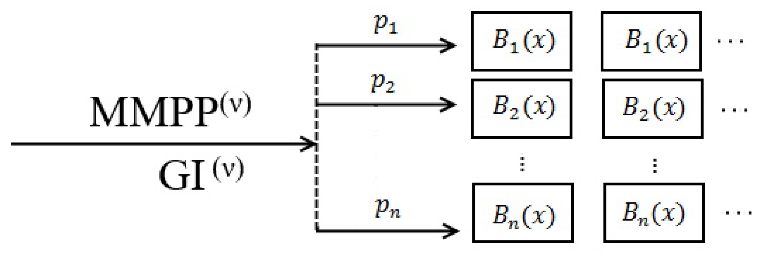
2. Mathematical Model of Resource Queues with Different Types of MMPP and Renewal Arrivals

Consider a queueing system with n different customers types and assume that each customer requests a random amount of resources (see Figure 1).

Customers arrive in the system according to a stochastic process (a Markov-modulated Poisson process (MMPP) or a renewal process). The MMPP process is given by the underlying Markov chain $k\left(t\right)$ with a finite number of states K, the set of non-negative intensities ${\lambda }_k$. Note that $k\left(t\right)$ is determined by the infinitesimal generator matrix $\mathbf{Q}=\left|q_{\nu k}\right|,\nu ,k=1,\dots ,K$. When the Markov chain $k\left(t\right)$ stays in the state $k,k=1,\dots ,K$, the customers arrive according to the stationary Poisson process with intensity ${\lambda }_k,k=1,\dots ,K$. The renewal arrival process is characterized by the distribution function $A\left(z\right)$ of the intervals between the arrivals’ moments.

At the time of occurrence of any event in the arrival process, only a single customer arrives in the system and its type is randomly selected according to the set of probabilities $p_i(i=1,\dots ,n)$. Then the customer goes to the appropriate device type, where its service is performed during a random time interval ${\xi }_i>0$ with the distribution function $B_i\left(x\right)=P\{{\xi }_i<x\}(i=1,\dots ,n)$ according to the type of the customer. Moreover, depending on its type, each customer requires a random amount of resources ${\nu }_i>0,i=1,\dots ,n$, drawn from the distribution function $G_i\left(y\right)=P\{{\nu }_i<y\}(i=1,\dots ,n)$, which is independent of its service time. Let us denote by $V_i\left(t\right)$ the total amount of occupied resources of the i-th type $(i=1,\dots ,n)$ at time t. The goal is to find the stationary probability distribution of the n-dimensional random process $\{V_1\left(t\right),V_2\left(t\right),\dots ,V_n\left(t\right)\}$. However, this process is non-Markovian; therefore, we will use the dynamic screening method for the investigation of this problem [32,36]. Let the system be empty at moment $t_0$, and let us fix any moment T in the future. The set of dynamic probabilities $S_i\left(t\right)=p_i(1-B_i(T-t))$$(i=1,\dots ,n)$ indicates that a customer arriving at time t has the i -type and it has not finished servicing at the moment T for $t_0\le t\le T$. We will consider such customers screened.

For resource queueing systems, we denote the amount of resources allocated by the original request that arrived at time instant t and screened by $W_i\left(t\right)$ and $(i=1,\dots ,n)$. Then the probability distribution of the amount of resources allocated in the system at time instant T coincides with the probability distribution in the screened process. The main idea of the dynamic screening method is to analyze the n-dimensional process $\{W_1\left(t\right),\dots ,W_n\left(t\right)\}$ and, substituting $t=T$, we obtain a result for the process $\{V_1\left(t\right),\dots ,V_n\left(t\right)\}$ at the time instant T.

It is easy to prove this property for the probability distribution of stochastic processes [34]:

$$P\{V_1\left(T\right)<w_1,\dots ,V_n\left(T\right)<w_n\}=P\{W_1\left(T\right)<w_1,...,W_n\left(T\right)<w_n\},w_i\ge 0,i=1,\dots n.$$

The resulting n-dimensional stochastic processes are also non-Markovian. Thus, we add the state of the Markov chain $k\left(t\right)$ for a system with an MMPP-flow and a residual time from t to the next arrival $z\left(t\right)$ for system with the renewal arrival process.

3. Kolmogorov Integro-Differential Equations

We can write systems of Kolmogorov integral differential equations to obtain the probability distribution of the resulting $(n+1)$-dimensional Markovian processes.

3.1. For System with MMPP Arrival Process

The probability distribution of the process $\{k\left(t\right),W_1\left(t\right),\dots ,W_n\left(t\right)\}$ is

$$\begin{array}{c}P(k,w_1,\dots ,w_n,t)=P\{k\left(t\right)=k,W_1\left(t\right)<w_1,\dots ,W_n\left(t\right)<w_n\},k=1,\dots ,K,\\ w_1>0,\dots ,w_n>0.\end{array}$$

Taking into account the formula of the total probability, we can write the following system of Kolmogorov differential equations:

$$\begin{array}{c}\frac{\partial P(k,w_1,\dots ,w_n,t)}{\partial t}={\displaystyle \sum _{\nu =1}^K}P(\nu ,w_1,\dots ,w_n,t)q_{\nu k}+\\ +{\displaystyle \sum _{i=1}^n}{\lambda }_k\left[(1-S_i\left(t\right))P(k,w_1,\dots ,w_n,t)+S_i\left(t\right)\underset{0}{\overset{w_i}{\int }}P(k,w_1,\dots ,w_i-y,\dots ,w_n,t)d{G}_i\left(y\right)\right],\\ k=1,\dots ,K.\end{array}$$

(1)

We introduce the partial characteristic function

$$h(k,u_1,\dots ,u_n,t)=\underset{0}{\overset{\infty }{\int }}{e}^{j{w}_1{u}_1}\cdots \underset{0}{\overset{\infty }{\int }}{e}^{j{w}_n{u}_n}P(k,d{w}_1,\dots ,d{w}_n,t),$$

where $j=\sqrt{-1}$ is the imaginary unit.

Then we can write the following equations:

$$\begin{array}{c}\frac{\partial h(k,u_1,\dots ,u_n,t)}{\partial t}={\lambda }_{k}h(k,u_1,\dots ,u_n,t){\displaystyle \sum _{i=1}^n}{S}_i\left(t\right)\left[G^{*}\left(u_i\right)-1\right]+\\ +{\displaystyle \sum _{\nu =1}^K}h(\nu ,u_1,\dots ,u_n,t)q_{\nu k},k=1,\dots ,K,\end{array}$$

(2)

where

$$G^{*}\left(u_i\right)=\underset{0}{\overset{\infty }{\int }}{e}^{j{u}_{i}y}d{G}_i\left(y\right),i=1,\dots ,n.$$

(3)

Then we can write the vector-matrix equation

$$\begin{array}{c}\frac{\partial \mathbf{h}(u_1,\dots ,u_n,t)}{\partial t}=\mathbf{h}(u_1,\dots ,u_n,t)\left[Q+{\displaystyle \sum _{i=1}^n}{S}_i\left(t\right)\left\{G^{*}\left(u_i\right)-1\right\}\mathbf{\Lambda }\right],\\ \mathbf{h}(u_1,\dots ,u_n,t_0)=\mathbf{r},\end{array}$$

(4)

where $\mathbf{h}(u_1,\dots ,u_n,t)=[h(1,u_1,\dots ,u_n,t),h(2,u_1,\dots ,u_n,t),\dots ,h(K,u_1,\dots ,u_n,t)]$ and $\mathbf{r}=\left[r\right(1),r(2),\dots ,r(K\left)\right]$ is the vector of the stationary probability distribution of the underlying Markov chain, defined by the following system of linear equations:

$$\{\begin{array}{c}\mathbf{r}\mathbf{Q}=0,\\ \mathbf{r}\mathbf{e}=1,\end{array}$$

(5)

$e={\left(\begin{array}{c}1\\ 1\\ ⋮\\ 1\end{array}\right)}_{1\times K}$, $\mathbf{\Lambda }=\left(\begin{array}{cccc}{\lambda }_1& 0& \dots & 0\\ 0& {\lambda }_2& \dots & 0\\ ⋮& ⋮& \ddots & ⋮\\ 0& 0& \dots & {\lambda }_K\end{array}\right)$.

3.2. For a System with a Renewal Arrival Process

The probability distribution of process $\{z\left(t\right),W_1\left(t\right),\dots ,W_n\left(t\right)\}$ is

$$P(z,w_1,\dots ,w_n,t)=P\{z\left(t\right)<z,W_1\left(t\right)<w_1,\dots ,W_n\left(t\right)<w_n\},z>0,w_1>0,\dots ,w_n>0.$$

The system of Kolmogorov differential equations has the form

$$\begin{array}{c}\frac{\partial P(z,w_1,\dots ,w_n,t)}{\partial t}=\frac{\partial P(z,w_1,\dots ,w_n,t)}{\partial z}+\frac{\partial P(0,w_1,\dots ,w_n,t)}{\partial z}(A\left(z\right)-1)+\\ +A\left(z\right){\displaystyle \sum _{i=1}^n}{S}_i\left(t\right)\left[{\displaystyle \underset{0}{\overset{w_i}{\int }}}\frac{\partial P(0,w_1,\dots ,w_i-y_i,\dots ,w_n,t)}{\partial z}d{G}_i\left(y\right)-\frac{\partial P(0,w_1,\dots ,w_n,t)}{\partial z}\right].\end{array}$$

(6)

We define the initial conditions in the form

$$P(z,w_1,\dots ,w_n,t_0)=\left\{\begin{array}{c}R\left(z\right),\mathrm{if}{w}_1=\cdots =w_n=0,\hfill \\ 0,\mathrm{otherwise},\hfill \end{array}\right.$$

where $R\left(z\right)$ is the stationary probability distribution of the stochastic process $z\left(t\right)$:

$$R\left(z\right)=\lambda \underset{0}{\overset{z}{\int }}(1-A\left(x\right))dx,a=\underset{0}{\overset{\infty }{\int }}(1-A\left(x\right))dx,\lambda =\frac{1}{a}.$$

(7)

Let us introduce the partial characteristic function

$$h(z,u_1,\dots ,u_n,t)=\underset{0}{\overset{\infty }{\int }}{e}^{j{u}_1{w}_1}\cdots \underset{0}{\overset{\infty }{\int }}{e}^{j{u}_n{w}_n}P(z,d{w}_1,\dots ,d{w}_n,t),z>0,$$

then, we obtain the following equation:

$$\begin{array}{c}\frac{\partial h(z,u_1,\dots ,u_n,t)}{\partial t}=\frac{\partial h(z,u_1,\dots ,u_n,t)}{\partial z}+\\ +\frac{\partial h(0,u_1,\dots ,u_n,t)}{\partial z}\left[A\left(z\right)-1+A\left(z\right){\displaystyle \sum _{i=1}^n}{S}_i\left(t\right)(G^{*}\left(u_i\right)-1)\right],\\ h(z,u_1,\dots ,u_n,t_0)=R\left(z\right),\end{array}$$

(8)

where $G^{*}\left(u_i\right)$ has form (3).

4. Gaussian Approximation of the Probability Distribution of the Total Resource Amounts

It was previously proven that under the asymptotic condition of an infinitely growing service time

• For resource queue $MMPP/GI\left(2\right)/\infty$: the joint probability distribution of the number of customers and total capacities is a multidimensional Gaussian distribution [34];
• For resource queue $GI/G{I}^{\left(n\right)}/\infty$: the n-dimensional probability distribution of the total resource amounts is asymptotically Gaussian [29].

To construct a Gaussian approximation of the distribution function of the random process $\{V_1\left(t\right),V_2\left(t\right),\dots ,V_n\left(t\right)\}$, we use the method of asymptotic analysis with the asymptotic conditions of the growing intensity of the arrival process. In the models under consideration, the flow intensity is represented as $N\lambda$, where $\lambda$ is a fixed value and the parameter N has large values (in theoretical studies $N\to \infty$). The value of N will be called the parameter of high flow intensity [37].

• For MMPP: to represent matrix of intensity $\mathbf{\Lambda }$ as ${\mathbf{\Lambda }}_1=N\mathbf{\Lambda }=\left(\begin{array}{cccc}N{\lambda }_1& 0& \dots & 0\\ 0& N{\lambda }_2& \dots & 0\\ ⋮& ⋮& \ddots & ⋮\\ 0& 0& \dots & N{\lambda }_K\end{array}\right)$ and the infinitesimal generator matrix Q as ${\mathbf{Q}}_1=N\mathbf{Q}$;
• For renewal arrivals: let us represent $t=\frac{\xi }{N},$ where $\xi$ is some non-negative random variable with the distribution function $A\left(z\right)$. Value $N>0$ is a parameter of high flow intensity, the meaning of which is described above. Then for the distribution function of interval lengths t, we have [38,39]

  $$P\{t<x\}=P\{\frac{\xi }{N}<x\}=P\{\xi <Nx\}=A\left(Nx\right).$$

  (9)
  Then Equation (6) is transformed into

  $$\begin{array}{c}\frac{1}{N}\frac{\partial P(z,w_1,\dots ,w_n,t)}{\partial t}=\frac{\partial P(z,w_1,\dots ,w_n,t)}{\partial z}+\frac{\partial P(0,w_1,\dots ,w_n,t)}{\partial z}(A\left(z\right)-1)+\\ +A\left(z\right){\displaystyle \sum _{i=1}^n}{S}_i\left(t\right)\left[\underset{0}{\overset{w_i}{\int }}\frac{\partial P(0,w_1,\dots ,w_i-y_i,\dots ,w_n,t)}{\partial z}d{G}_i\left(y\right)-\frac{\partial P(0,w_1,\dots ,w_n,t)}{\partial z}\right].\end{array}$$

  (10)
  Equation (8), in turn, takes the form

  $$\begin{array}{c}\frac{1}{N}\frac{\partial h(z,u_1,\dots ,u_n,t)}{\partial t}=\frac{\partial h(z,u_1,\dots ,u_n,t)}{\partial z}+\\ +\frac{\partial h(0,u_1,\dots ,u_n,t)}{\partial z}\left[A\left(z\right)-1+A\left(z\right){\displaystyle \sum _{i=1}^n}{S}_i\left(t\right)(G^{*}\left(u_i\right)-1)\right],\\ h(z,u_1,\dots ,u_n,t_0)=R\left(z\right).\end{array}$$

  (11)

We state and prove the following theorems.

Theorem 1.

Under the condition of the growing intensity of the arrival process, the joint asymptotic probability distribution of the n-dimensional process of the total amounts of the occupied resources in the heterogeneous QS is the n-dimensional Gaussian distribution with parameters that are dependent on the type of arrival process. The expectation vector has the form

$$\mathit{a}=N\lambda \left[\begin{array}{ccc}{a}_1{b}_1& \dots & a_n{b}_n\end{array}\right],$$

(12)

and the covariance matrix has the form

$$\mathit{K}=N(\lambda {\mathit{K}}^{\left(1\right)}+\kappa {\mathit{K}}^{\left(2\right)}).$$

(13)

Here

$$\begin{array}{c}{\mathbf{K}}^{\left(1\right)}=\left[\begin{array}{ccc}{d}_1{b}_1& \cdots & 0\\ \cdots & \cdots & \cdots \\ 0& \cdots & d_n{b}_n\end{array}\right],{\mathbf{K}}^{\left(2\right)}=\left[\begin{array}{ccc}{\beta }_{11}{a}_1{a}_1& \cdots & {\beta }_{1n}{a}_1{a}_n\\ \cdots & \cdots & \cdots \\ {\beta }_{n1}{a}_n{a}_1& \cdots & {\beta }_{nn}{a}_n{a}_n\end{array}\right],\\ a_i=\underset{0}{\overset{\infty }{\int }}yd{G}_i\left(y\right),d_i=\underset{0}{\overset{\infty }{\int }}{y}^{2}d{G}_i\left(y\right),b_i=p_i\underset{0}{\overset{\infty }{\int }}(1-B_i\left(x\right))dx,\\ {\beta }_{ij}=p_i{p}_j\underset{0}{\overset{\infty }{\int }}(1-B_i\left(x\right))(1-B_j\left(x\right))dx,i=1,\dots ,n,j=1,\dots ,n,\end{array}$$

λ and κ are defined by the type of arrival process:

• For MMPP:

$$\lambda =\mathbf{r}\mathbf{\Lambda }\mathbf{e},\kappa =2\mathbf{g}\left(\mathbf{\Lambda }-\lambda \mathbf{I}\right)\mathbf{e},$$

(14)

$\mathbf{g}$ is the solution of system

$$\left\{\begin{array}{c}\mathbf{gQ}=\mathbf{r}\left(\lambda \mathbf{I}-\mathbf{\Lambda }\right),\\ \mathbf{ge}=0;\end{array}\right.$$

• For the renewal process:

$$\lambda ={\left(\underset{0}{\overset{\infty }{\int }}(1-A\left(x\right))dx\right)}^{-1},\kappa ={\lambda }^3\left({\sigma }^2-a^2\right),$$

(15)

where a and ${\sigma }^2$ are the expectation and variance of a random variable given by the distribution function $A\left(z\right)$, $\mathbf{I}={\left(\begin{array}{cccc}1& 0& \dots & 0\\ 0& 1& \dots & 0\\ ⋮& ⋮& \ddots & ⋮\\ 0& 0& \dots & 1\end{array}\right)}_{K\times K}.$

Proof of Theorem 1.

Step 1. For a system with MMPP.

Let us perform substitutions

$$\epsilon =\frac{1}{N},u_i=\epsilon x_i,i=1,\dots ,n,\mathbf{h}(u_1,\dots ,u_n,t)={\mathbf{f}}_1(x_1,\dots ,x_n,t,\epsilon ).$$

(16)

Then problem (4) takes the form

$$\begin{array}{c}\epsilon \frac{\partial {\mathbf{f}}_1(x_1,\dots ,x_n,t,\epsilon )}{\partial t}={\mathbf{f}}_1(x_1,\dots ,x_n,t,\epsilon )\left[\mathbf{Q}+{\displaystyle \sum _{i=1}^n}{S}_i\left(t\right)\left\{G^{*}\left(\epsilon x_i\right)-1\right\}\mathbf{\Lambda }\right],\\ {\mathbf{f}}_1(x_1,\dots ,x_n,t_0,\epsilon )=\mathbf{r}.\end{array}$$

(17)

Let $\epsilon \to 0$, then problem (17) has the form

$$\begin{array}{c}{\mathbf{f}}_1(x_1,\dots ,x_n,t)Q=0,\\ {\mathbf{f}}_1(x_1,\dots ,x_n,t_0)=\mathbf{r},\end{array}$$

and the asymptotic solution ${\mathbf{f}}_1(x_1,\dots ,x_n,t)$ of (17) should be searched in the following form:

$$\begin{array}{c}{\mathbf{f}}_1(x_1,\dots ,x_n,t)=\mathbf{r}{\Phi }_1(x_1,\dots ,x_n,t),\\ {\Phi }_1(x_1,\dots ,x_n,t_0)=1,\end{array}$$

(18)

where ${\Phi }_1(x_1,\dots ,x_n,t)$ is some scalar function.

We then substitute (18) into (17) and multiply the resulting equation by e. Then, given that $\mathbf{r}\mathbf{\Lambda }\mathbf{e}=\lambda$, we get

$$\epsilon \frac{\partial {\Phi }_1(x_1,\dots ,x_n,t)}{\partial t}=\lambda {\Phi }_1(x_1,\dots ,x_n,t)\sum _{i=1}^n{S}_i\left(t\right)\left\{G^{*}\left(\epsilon x_i\right)-1\right\}.$$

(19)

We use the expansion of the exponent in the Taylor series for $G^{*}\left(\epsilon x_i\right)$:

$$\begin{array}{c}{G}^{*}\left(\epsilon x_i\right)=\underset{0}{\overset{\infty }{\int }}{e}^{j\epsilon x_{i}y}d{G}_i\left(y\right)=\underset{0}{\overset{\infty }{\int }}\left(1+j\epsilon x_{i}y+O\left({\epsilon }^2\right)\right)d{G}_i\left(y\right)=\\ =1+j\epsilon x_i{a}_i+O\left({\epsilon }^2\right),\end{array}$$

(20)

where $a_i=\underset{0}{\overset{\infty }{\int }}yd{G}_i\left(y\right).$

Substituting this into (19) and then divide the resulting equation by $\epsilon (\epsilon \to 0)$, we derive

$$\frac{\partial {\Phi }_1(x_1,\dots ,x_n,t)}{\partial t}=j\lambda {\Phi }_1(x_1,\dots ,x_n,t)\sum _{i=1}^n{S}_i\left(t\right)x_i{a}_i.$$

(21)

The solution of the differential Equation (21) is

$${\Phi }_1(x_1,\dots ,x_n,t)=exp\left\{j\lambda \sum _{i=1}^n{x}_i{a}_i\underset{t_0}{\overset{t}{\int }}{S}_i\left(\tau \right)d\tau \right\}.$$

(22)

By performing back-substitutions and putting $t_0=-\infty ,T=t=0$, we can write the first-order asymptotic characteristic function $h_1(u_1,\dots ,u_n)$ in the form

$$\begin{array}{c}{h}_1(u_1,\dots ,u_n)={\mathbf{h}}_1(u_1,\dots ,u_n,0)\mathbf{e}\approx {\mathbf{f}}_1(x_1,\dots ,x_n,0)\mathbf{e}=\\ =\mathbf{r}exp\left\{j\lambda {\displaystyle \sum _{i=1}^n}{x}_i{a}_i\underset{-\infty }{\overset{0}{\int }}{S}_i\left(\tau \right)d\tau \right\}\mathbf{e}=exp\left\{jN\lambda {\displaystyle \sum _{i=1}^n}{u}_i{a}_i{b}_i\right\}.\end{array}$$

(23)

To construct the second-order asymptotic characteristic function ${\mathbf{h}}_2(u_1,\dots ,u_n,t)$, we represent the function $\mathbf{h}(u_1,\dots ,u_n,t)$ in the following form:

$$\mathbf{h}(u_1,\dots ,u_n,t)={\mathbf{h}}_2(u_1,\dots ,u_n,t)exp\left\{jN\lambda \sum _{i=1}^n{u}_i{a}_i{b}_i\right\}.$$

(24)

Substituting this expression into (4), we obtain the equation regarding ${\mathbf{h}}_2(u_1,\dots ,u_n,t)$

$$\begin{array}{c}\frac{1}{N}\frac{\partial {\mathbf{h}}_2(u_1,\dots ,u_n,t)}{\partial t}={\mathbf{h}}_2(u_1,\dots ,u_n,t)\left\{\mathbf{Q}+\sum _{i=1}^n{S}_i\left(t\right)\left[(G^{*}\left(u_i\right)-1)\mathbf{\Lambda }-j\lambda u_i{a}_i\mathbf{I}\right]\right\},\\ {\mathbf{h}}_2(u_1,\dots ,u_n,t_0)=\mathbf{r}.\end{array}$$

(25)

Let us use the following substitutions in (25):

$${\epsilon }^2=\frac{1}{N},u_i=\epsilon x_i,i=1,\dots ,n,{\mathbf{h}}_2(u_1,\dots ,u_n,t)={\mathbf{f}}_2(x_1,\dots ,x_n,t,\epsilon ).$$

$$\begin{array}{c}{\epsilon }^2\frac{\partial {\mathbf{f}}_2(x_1,\dots ,x_n,t,\epsilon )}{\partial t}={\mathbf{f}}_2(x_1,\dots ,x_n,t,\epsilon )\left\{\mathbf{Q}+\sum _{i=1}^n{S}_i\left(t\right)\left[(G^{*}\left(\epsilon x_i\right)-1)\mathbf{\Lambda }-j\lambda \epsilon x_i{a}_i\mathbf{I}\right]\right\},\\ {\mathbf{f}}_2(x_1,\dots ,x_n,t_0,\epsilon )=\mathbf{r}.\end{array}$$

(26)

Let us find the asymptotic solution ${\mathbf{f}}_2(x_1,\dots ,x_n,t)=\underset{\epsilon \to 0}{lim}{\mathbf{f}}_2(x_1,\dots ,x_n,t,\epsilon )$. Let $\epsilon \to 0$; then, Equation (26) becomes

$$\begin{array}{c}{\mathbf{f}}_2(x_1,\dots ,x_n,t)\mathbf{Q}=0,\\ {\mathbf{f}}_2(x_1,\dots ,x_n,t_0)=\mathbf{r}.\end{array}$$

We can represent the solution ${\mathbf{f}}_2(x_1,\dots ,x_n,t,\epsilon )$ of Equation (26) as

$$\begin{array}{c}{\mathbf{f}}_2(x_1,\dots ,x_n,t)=\mathbf{r}{\Phi }_2(x_1,\dots ,x_n,t),\\ {\Phi }_2(x_1,\dots ,x_n,t_0)=1.\end{array}$$

So, function ${\mathbf{f}}_2(x_1,\dots ,x_n,t)$ will take the form

$${\mathbf{f}}_2(x_1,\dots ,x_n,t,\epsilon )={\Phi }_2(x_1,\dots ,x_n,t)\left[\mathbf{r}+j\epsilon \sum _{i=1}^n{x}_i{a}_i{S}_i\left(t\right)g\right]+O\left({\epsilon }^2\right).$$

(27)

Substituting (27) into (26) we obtain

$$O\left({\epsilon }^2\right)={\Phi }_2(x_1,\dots ,x_n,t)\left[\mathbf{r}\mathbf{Q}+j\epsilon \sum _{i=1}^n{x}_i{a}_i{S}_i\left(t\right)\mathbf{r}[\mathbf{\Lambda }-\lambda \mathbf{I}]+j\epsilon \sum _{i=1}^n{x}_i{a}_i{S}_i\left(t\right)g\mathbf{Q}\right]=0,$$

where g is some row vector that satisfies the following system:

$$\left\{\begin{array}{c}\mathbf{gQ}=\mathbf{r}\left(\lambda \mathbf{I}-\mathbf{\Lambda }\right),\\ \mathbf{ge}=0.\end{array}\right.$$

We use the exponent expansion for functions in the form

$$\begin{array}{c}{G}^{*}\left(\epsilon x_i\right)=\underset{0}{\overset{\infty }{\int }}{e}^{j\epsilon x_{i}y}d{G}_i\left(y\right)=\underset{0}{\overset{\infty }{\int }}\left(1+j\epsilon x_{i}y+\frac{{\left(j\epsilon x_{i}y\right)}^2}{2}+O\left({\epsilon }^3\right)\right)d{G}_i\left(y\right)=\\ =1+j\epsilon x_i{a}_i+\frac{{\left(j\epsilon x_i\right)}^2}{2}{d}_i+O\left({\epsilon }^3\right),\end{array}$$

(28)

here $d_i=\underset{0}{\overset{\infty }{\int }}{y}^{2}d{G}_{(}y).$

Next, let $\epsilon \to 0$. Taking into account (26), (27) takes the form

$$\begin{array}{c}{\Phi }_2(x_1,\dots ,x_n,t)=exp\left\{\lambda \sum _{i=1}^n\frac{j^2{x}_i^2}{2}{d}_i\underset{t_0}{\overset{t}{\int }}{S}_i\left(\tau \right)d\tau +\kappa \sum _{i=1}^n{j}^2{x}_i^2{a}_i^2\underset{t_0}{\overset{t}{\int }}{S}_i^2\left(\tau \right)d\tau \right\},\\ {\Phi }_2(x_1,\dots ,x_n,t_0)=1.\end{array}$$

We assume that $t_0=-\infty ,T=t=0$; then, function $\mathbf{h}(u_1,\dots ,u_n,0)$ will have the form

$$\begin{array}{c}\mathbf{h}(u_1,\dots ,u_n,0)={\mathbf{h}}_2(u_1,\dots ,u_n,0)exp\left\{jN\lambda {\displaystyle \sum _{i=1}^n}{u}_i{a}_i{b}_i\right\}=\\ =\mathbf{r}exp\left\{jN\lambda {\displaystyle \sum _{i=1}^n}{u}_i{a}_i{b}_i+\lambda N{\displaystyle \sum _{i=1}^n}\frac{j^2{u}_i^2}{2}{d}_i{b}_i+N\kappa {\displaystyle \sum _{i=1}^n}{j}^2{u}_i^2{a}_i^2{\beta }_i\right\}.\end{array}$$

(29)

Therefore, the second-order asymptotic of the characteristic function has the form

$$h(u_1,\dots ,u_n)=\mathbf{h}(u_1,\dots ,u_n,0)e=\mathbf{r}exp\left\{jN\lambda \sum _{i=1}^n{u}_i{a}_i{b}_i+\frac{j^2}{2}N\lambda \sum _{i=1}^n{d}_i{b}_i+j^{2}N\kappa \sum _{i=1}^n{u}_i^2{a}_i^2{\beta }_i\right\}.$$

(30)

Step 2. For a system with renewal arrival process.

Let us make the following substitutions in (11)

$$\epsilon =\frac{1}{N},u_i=\epsilon x_i,i=1,\dots ,n,h(z,u_1,\dots ,u_n,t)=f_1(z,x_1,\dots ,x_n,t,\epsilon ).$$

(31)

We obtain

$$\begin{array}{c}\epsilon \frac{\partial f_1(z,x_1,\dots ,x_n,t,\epsilon )}{\partial t}=\frac{\partial f_1(z,x_1,\dots ,x_n,t,\epsilon )}{\partial z}+\\ +\frac{\partial f_1(0,x_1,\dots ,x_n,t,\epsilon )}{\partial z}\left[A\left(z\right)-1+A\left(z\right){\displaystyle \sum _{i=1}^n}{S}_i\left(t\right)(G^{*}\left(\epsilon x_i\right)-1)\right],\\ f_1(z,x_1,\dots ,x_n,t_0,\epsilon )=R\left(z\right),\end{array}$$

(32)

To find the first-order asymptotic solution

$$f_1(z,x_1,\dots ,x_n,t)=\underset{\epsilon \to 0}{lim}{f}_1(z,x_1,\dots ,x_n,t,\epsilon ),$$

let $\epsilon \to 0$ in (32):

$$\frac{\partial f_1(z,x_1,\dots ,x_n,t)}{\partial z}+\frac{\partial f_1(0,x_1,\dots ,x_n,t)}{\partial z}\left[A\left(z\right)-1\right]=0.$$

We assume that

$$\begin{array}{c}{f}_1(z,x_1,\dots ,x_n,t)=R\left(z\right){\Phi }_1(x_1,\dots ,x_n,t),\\ {\Phi }_1(x_1,\dots ,x_n,t_0)=1,\end{array}$$

(33)

where ${\Phi }_1(x_1,\dots ,x_n,t)$ is a scalar differentiable function.

Let $z\to \infty$ in (32):

$$\epsilon \frac{\partial f_1(\infty ,x_1,\dots ,x_n,t,\epsilon )}{\partial t}=\frac{\partial f_1(0,x_1,\dots ,x_n,t,\epsilon )}{\partial z}\sum _{i=1}^n{S}_i\left(t\right)(G^{*}\left(\epsilon x_i\right)-1).$$

(34)

We use the exponent expansion for functions in the form of (20) and substitute (33) into (34). Furthermore, we divide the resulting expression by $\epsilon$ and let $\epsilon \to 0$

$$\frac{\partial {\Phi }_1(x_1,\dots ,x_n,t)}{\partial t}={\Phi }_1(x_1,\dots ,x_n,t)j\lambda \sum _{i=1}^n{x}_i{a}_i{S}_i\left(t\right).$$

(35)

It is easy to see that the solution of Equation (35) is

$${\Phi }_1(x_1,\dots ,x_n,t)=exp\left\{j\lambda {\displaystyle \sum _{i=1}^n}{x}_i{a}_i\underset{t_0}{\overset{t}{\int }}{S}_i\left(\tau \right)d\tau \right\}.$$

(36)

Furthermore, similarly to the earlier reasoning for the case with an incoming MMPP, we obtain the form of the first-order asymptotic characteristic function $\mathbf{h}(z,u_1,\dots ,u_n,t)$

$$h(z,u_1,\dots ,u_n,t)=R\left(z\right)exp\left\{jN\lambda {\displaystyle \sum _{i=1}^n}{u}_i{a}_i\underset{t_0}{\overset{t}{\int }}{S}_i\left(\tau \right)d\tau \right\}.$$

(37)

Let us proceed to the construction of the second-order asymptotic. We introduce the function

$$h(z,u_1,\dots ,u_n,t)=h_2(z,u_1,\dots ,u_n,t)exp\left\{jN\lambda {\displaystyle \sum _{i=1}^n}{u}_i{a}_i\underset{t_0}{\overset{t}{\int }}{S}_i\left(\tau \right)d\tau \right\}.$$

(38)

In (11), let us make substitutions

$${\epsilon }^2=\frac{1}{N},u_i=\epsilon x_i,i=1,\dots ,n,h_2(z,u_1,\dots ,u_n,t)=f_2(z,x_1,\dots ,x_n,t,\epsilon )$$

(39)

and, given (38), we obtain

$$\begin{array}{c}{\epsilon }^2\frac{\partial f_2(z,x_1,\dots ,x_n,t,\epsilon )}{\partial t}+f_2(z,x_1,\dots ,x_n,t,\epsilon )j\epsilon \lambda \sum _{i=1}^n{x}_i{a}_i{S}_i\left(t\right)=\frac{\partial f_2(z,x_1,\dots ,x_n,t,\epsilon )}{\partial z}+\\ +\frac{\partial f_2(0,x_1,\dots ,x_n,t,\epsilon )}{\partial z}\left[A\left(z\right)-1+A\left(z\right){\displaystyle \sum _{i=1}^n}{S}_i\left(t\right)(G^{*}\left(\epsilon x_i\right)-1)\right].\end{array}$$

(40)

Let us find the asymptotic solution of Equation (40)

$$f_2(z,x_1,\dots ,x_n,t)=\underset{\epsilon \to 0}{lim}{\mathbf{f}}_2(z,x_1,\dots ,x_n,t,\epsilon ).$$

(41)

So,

$$\frac{\partial f_2(z,x_1,\dots ,x_n,t)}{\partial z}+\frac{\partial f_2(0,x_1,\dots ,x_n,t,\epsilon )}{\partial z}\left[A\left(z\right)-1\right]=0.$$

(42)

We find the function $f_2(z,x_1,\dots ,x_n,t)$ as follows:

$$\begin{array}{c}{f}_2(z,x_1,\dots ,x_n,t)=R\left(z\right){\Phi }_2(x_1,\dots ,x_n,t),\\ {\Phi }_2(x_1,\dots ,x_n,t_0)=1.\end{array}$$

(43)

We write the function $f_2(z,x_1,\dots ,x_n,t)$ as the power expansion

$$\begin{array}{c}{f}_2(z,x_1,\dots ,x_n,t,\epsilon )={\Phi }_2(x_1,\dots ,x_n,t)\left[R\left(z\right)+j\epsilon \lambda f\left(z\right){\displaystyle \sum _{i=1}^n}{x}_i{a}_i{S}_i\left(t\right)+O\left({\epsilon }^2\right)\right],\end{array}$$

(44)

where $f\left(z\right)$ is some differentiable function.

We substitute (44) into (42) and derive a differential equation for the unknown function $f\left(z\right)$:

$$\begin{array}{c}f\left(z\right)=f^{\prime }\left(0\right)\underset{0}{\overset{z}{\int }}(1-A\left(x\right))dx+\underset{0}{\overset{z}{\int }}(R\left(x\right)-A\left(x\right))dx.\end{array}$$

In Equation (42), we make the transition to the limit $z\to \infty$. The function $f_2(z,x_1,\dots ,x_n,$$t,\epsilon )$ is monotonically increasing and bounded above at z, then:

$$\begin{array}{c}\underset{z\to \infty }{lim}\frac{\partial f_2(z,x_1,\dots ,x_n,t,\epsilon )}{\partial z}=0.\end{array}$$

In (40) we use the exponent expansion for functions in form of (28), then for $z\to \infty$, we obtain

$$\begin{array}{c}{\epsilon }^2\frac{\partial f_2(\infty ,x_1,\dots ,x_n,t,\epsilon )}{\partial t}+f_2(\infty ,x_1,\dots ,x_n,t,\epsilon )j\epsilon \lambda {\displaystyle \sum _{i=1}^n}{x}_i{a}_i{S}_i\left(t\right)=\frac{\partial f_2(\infty ,x_1,\dots ,x_n,t,\epsilon )}{\partial z}+\\ +\frac{\partial f_2(0,x_1,\dots ,x_n,t,\epsilon )}{\partial z}{\displaystyle \sum _{i=1}^n}{S}_i\left(t\right)\left(j\epsilon x_i{a}_i+\frac{{\left(j\epsilon x_i\right)}^2}{2}{d}_i\right)+O\left({\epsilon }^3\right).\end{array}$$

(45)

By substituting (44) into the obtained expression, let us divide everything by ${\epsilon }^2(\epsilon \to 0)$. Then, taking into account the fact that $\kappa =2f^{\prime }\left(0\right)-2f(\infty )$, let $f(\infty )=const$. Putting $f(\infty )=0$, we can observe that $\kappa =2f^{\prime }\left(0\right)$ and obtain the equation for ${\Phi }_2(x_1,\dots ,x_n,t)$:

$$\frac{\partial {\Phi }_2(x_1,\dots ,x_n,t)}{\partial t}={\Phi }_2(x_1,\dots ,x_n,t)\left[\lambda \sum _{i=1}^n\frac{{\left(j{x}_i\right)}^2}{2}{d}_i{S}_i\left(t\right)+\kappa \sum _{i=1}^n\sum _{m=1}^n\frac{\left(j{x}_i\right)\left(j{x}_m\right)}{2}{a}_i{a}_m{S}_i\left(t\right)S_m\left(t\right)\right].$$

The solution of the differential equation is

$$\begin{array}{c}{\Phi }_2(x_1,\dots ,x_n,t)=exp\left\{\lambda {\displaystyle \sum _{i=1}^n}\frac{{\left(j{x}_i\right)}^2}{2}{d}_i{\displaystyle \underset{t_0}{\overset{t}{\int }}}{S}_1\left(\tau \right)d\tau +\kappa {\displaystyle \sum _{i=1}^n}\sum _{m=1}^n\frac{\left(j{x}_i\right)\left(j{x}_m\right)}{2}{a}_i{a}_m\underset{t_0}{\overset{t}{\int }}{S}_i\left(\tau \right)S_m\left(\tau \right)d\tau \right\}.\end{array}$$

(46)

We substitute (46) in (43), then, following the reverse substitutions, we write the approximate asymptotic equality regarding $h(z,u_1,\dots ,u_n,t)$. □

5. Simulation and Numerical Analysis

The aim of numerical and simulation experiments is to determine the limits of applicability of the obtained Gaussian approximation of the distribution function.

Let us consider as an input an MMPP with the following parameters:

$$\begin{array}{c}\mathbf{\Lambda }=\left[\begin{array}{ccc}0.5& 0& 0\\ 0& 1& 0\\ 0& 0& 1.5\end{array}\right],\mathbf{Q}=\left[\begin{array}{ccc}-0.8& 0.4& 0.4\\ 0.3& -0.6& 0.3\\ 0.4& 0.4& -0.8\end{array}\right].\end{array}$$

For the renewal arrival process, the intervals between the arrivals have a uniform distribution over the interval $[0.5,1.5]$.

The type of an incoming customer is defined as i-type with probabilities of $p_1=0.5$, $p_2=0.3$, $p_3=0.2.$ 

Table 1. The laws of parameter distributions for systems of various types.

Type of System	Volume	Service Time
First	Geometric $\left(0.2\right)$	Gamma $(0.5,0.5)$
Second	Poisson $\left(3\right)$	Exponential $\left(1\right)$
Third	Binomial $(0.5,12)$	Uniform $(0.1,0.9)$

shows the distribution laws of the random variables which characterize the amount of occupied resources and the time required to service the customers.

By means of a simulation, we obtained the marginal empirical probability distribution functions for the total numbers of resources occupied by each type of customer. Our goal was to compare the empirical and asymptotic distribution laws. To this end, we used the Kolmogorov distance: ${\Delta }_i={sup}_x\left|F_{em}\left(x\right)-F_{as}\left(x\right)\right|,i=1,\dots ,3$, where the subscript “em” denotes the empirical distribution function built on the simulation results and “as” denotes the asymptotic distribution function based on the theorem.

Table 2. Kolmogorov distances, comparing simulation results and asymptotic values for the total capacity of customers of different types for the QS MMPP${}^{\left(\nu \right)}$|GI|∞. Bold format highlights results that do not exceed the value of the acceptable approximation threshold.

N	5	10	20	30	60	100	200	300	500
${\Delta }_1$	$0.163$	$0.088$	$\mathbf{0}.\mathbf{048}$	$\mathbf{0}.\mathbf{036}$	$\mathbf{0}.\mathbf{025}$	$\mathbf{0}.\mathbf{019}$	$\mathbf{0}.\mathbf{013}$	$\mathbf{0}.\mathbf{011}$	$\mathbf{0}.\mathbf{008}$
${\Delta }_2$	$0.185$	$0.091$	$\mathbf{0}.\mathbf{047}$	$\mathbf{0}.\mathbf{034}$	$\mathbf{0}.\mathbf{022}$	$\mathbf{0}.\mathbf{017}$	$\mathbf{0}.\mathbf{012}$	$\mathbf{0}.\mathbf{010}$	$\mathbf{0}.\mathbf{007}$
${\Delta }_3$	$0.326$	$0.121$	$0.054$	$\mathbf{0}.\mathbf{037}$	$\mathbf{0}.\mathbf{022}$	$\mathbf{0}.\mathbf{017}$	$\mathbf{0}.\mathbf{013}$	$\mathbf{0}.\mathbf{010}$	$\mathbf{0}.\mathbf{007}$

and

Table 3. Kolmogorov distances, comparing simulation results and asymptotic values for the total capacity of customers of different types for the QS GI${}^{\left(\nu \right)}$|GI|∞. Bold format highlights results that do not exceed the value of the acceptable approximation threshold.

N	5	10	20	30	60	100	200	300	500
${\Delta }_1$	$0.148$	$0.079$	$\mathbf{0}.\mathbf{044}$	$\mathbf{0}.\mathbf{034}$	$\mathbf{0}.\mathbf{024}$	$\mathbf{0}.\mathbf{018}$	$\mathbf{0}.\mathbf{013}$	$\mathbf{0}.\mathbf{011}$	$\mathbf{0}.\mathbf{008}$
${\Delta }_2$	$0.158$	$0.077$	$\mathbf{0}.\mathbf{039}$	$\mathbf{0}.\mathbf{029}$	$\mathbf{0}.\mathbf{019}$	$\mathbf{0}.\mathbf{015}$	$\mathbf{0}.\mathbf{011}$	$\mathbf{0}.\mathbf{009}$	$\mathbf{0}.\mathbf{007}$
${\Delta }_3$	$0.296$	$0.101$	$\mathbf{0}.\mathbf{042}$	$\mathbf{0}.\mathbf{029}$	$\mathbf{0}.\mathbf{018}$	$\mathbf{0}.\mathbf{014}$	$\mathbf{0}.\mathbf{010}$	$\mathbf{0}.\mathbf{008}$	$\mathbf{0}.\mathbf{007}$

show values of the Kolmogorov distances for the total volumes of the occupied resources of each type. The accuracy of the approximation increases with an increase in the mean of the system load, so, even with $N=30$ for MMPP and $N=20$ for renewal arrival process, the value of ${\Delta }_i,i=1,2,3,$ does not exceed $0.05$.

We can use the results presented in Section 4 in the case of a system with limited resources. For example, for the task of choosing the optimal values of resources provided in each channel. These limit values should provide a given probability of losing requests due to a lack of resources to service them. Denote by $V_k^{opt}$ the optimal volume of the k-th channel. The estimation of these values is based on the Gaussian distribution (Theorem 1) and the method described in [40] and has the form:

$$V_k^{opt}=a_k+r\sqrt{K_{kk}}.$$

(47)

Here r is the so-called hyper-ellipsoid radius, which depends on $p_{loss}$ and which can be evaluated using the method described in [40].

6. Conclusions

In this study, we considered the problem of analyzing the total amount of resources allocated in queueing systems with different nodes for the processing of heterogeneous data that require arbitrary resource capacities for their service. We applied the methods of dynamic screening and the asymptotic analysis to obtain an approximation of the stationary probability distribution of the total occupied resource amount. As a result of this study, we can conclude that the total resource amounts of the occupied resources in a heterogeneous queueing system with parameters dependent on the condition of a high load have a multidimensional Gaussian distribution. Their parameters (mean vector and covariance matrix) were also obtained. The comparison of the asymptotic results with the simulation results showed that the accuracy of the presented approach was sufficiently high. Furthermore, we have demonstrated how the results of the approximations can be applied to estimating the optimal total resource amount for a system with a limited amount of resources. The approach presented in this paper may be applied to the study of resource queues with the splitting of requests, as well as systems with the arrival processes of other types (e.g., a batch Markovian arrival process, a semi-Markov process, etc.).

References

1. Dudin, A.N.; Klimenok, V.I.; Vishnevsky, V.M. The Theory of Queueing Qystems with Correlated Flows; Springer: Berlin/Heidelberg, Germany, 2020; 410p. [Google Scholar]
2. Lakatos, L.; Szeidl, L.; Miklos, T. Introduction to Queueing Systems with Telecommunication Applications; Springer: Boston, MA, USA, 2013; 388p. [Google Scholar]
3. Stepanov, S.N. Fundamentals of Teletraffic Multiservice Networks; Eco-Trends: Moscow, Russia, 2010. (In Russian) [Google Scholar]
4. Stepanov, S.N. The Theory of Teletraffic. Concepts, Models, Applications; Goryachaya Liniya: Moscow, Russia, 2016. (In Russian) [Google Scholar]
5. Romm, E.L.; Skitovich, V.V. On a generalization of the Erlang problem. Autom. Remote Control 1971, 6, 164–168. (In Russian) [Google Scholar]
6. Gorbunova, A.V.; Naumov, V.A.; Gaidamaka, Y.V.; Samouylov, K.E. Resource queueing systems as models of wireless communication systems. Inform. Appl. 2021, 12, 48–55. [Google Scholar]
7. Samouylov, K.; Sopin, E.; Vikhrova, O. Analysis of queueing system with resources and signals. In Proceedings of the International Conference on Information Technologies and Mathematical Modelling, Kazan, Russia, 29 September–3 October 2017; Springer: Berlin/Heidelberg, Germany, 2017; Volume 800, pp. 358–369. [Google Scholar]
8. Sopin, E.; Vikhrova, O.; Samouylov, K. LTE network model with signals and random resource requirement. In Proceedings of the 9th Congress (International) on Ultra Modern Telecommunications and Control Systems and Workshops, Munich, Germany, 6–8 November 2017; pp. 101–106. [Google Scholar]
9. Tikhonenko, O.M. Distribution of the total volume of messages in a single-server queueing system with group arrival. Autom. Remote Control 1985, 46, 1412–1416. [Google Scholar]
10. Tikhonenko, O.M. Queueing Models in Information Processing Systems; BSU Publishing House: Minsk, Belarus, 1990. (In Russian) [Google Scholar]
11. Tikhonenko, O.; Kempa, W.M. On the queue-size distribution in the multi-server system with bounded capacity and packet dropping. Kybernetika 2013, 49, 855–867. [Google Scholar]
12. Tikhonenko, O.; Kempa, W.M. Performance evaluation of an M/G/n-type queue with bounded capacity and packet dropping. Int. J. Appl. Math. Comput. Sci. 2016, 26, 841–854. [Google Scholar] [CrossRef]
13. Klimenok, V.I.; Dudin, A.N.; Vishnevsky, V.M. Priority Multi-Server Queueing System with Heterogeneous Customers. Mathematics 2020, 8, 1501. [Google Scholar] [CrossRef]
14. Moskaleva, F.; Lisovskaya, E.; Gaidamaka, Y. Resource Queueing System for Analysis of Network Slicing Performance with QoS-Based Isolation. In Proceedings of the International Conference on Information Technologies and Mathematical Modelling, Tomsk, Russia, 1–5 December 2021; Springer: Berlin/Heidelberg, Germany, 2021; Volume 1391, pp. 198–211. [Google Scholar]
15. Naumov, V.; Samouylov, K. Resource System with Losses in a Random Environment. Mathematics 2021, 9, 2685. [Google Scholar] [CrossRef]
16. Lucantoni, D.M. New results on single server queue with a batch Markovian arrival process. Commun. Stat. Stoch. Model. 1991, 7, 1–46. [Google Scholar] [CrossRef]
17. Neuts, M.F. Models based on the Markovian arrival process. IEICE Trans. Commun. 1992, 75, 1255–1265. [Google Scholar]
18. Nazarov, A.A.; Moiseeva, S.P. Asymptotic Analysis Method in Queuing Theory; NTL: Tomsk, Russia, 2006. (In Russian) [Google Scholar]
19. Bartlett, M.S. Some evolutionary stochastic processes. J. R. Stat. Soc. Ser. B 1949, 11, 211–229. [Google Scholar] [CrossRef]
20. Benes, V.E. Mathematical Theory of Connecting Networks and Telephone Traffic; Academic Press: New York, NY, USA, 1965. [Google Scholar]
21. Cramer, H.; Leadbetter, M.R. Stationary and Related Stochastic Processes; Wiley: New York, NY, USA, 1967. [Google Scholar]
22. Palm, C. The Distribution of Repairmen in Servicing Automatic Machines. Ind. Nord. 1947, 75, 75–80. [Google Scholar]
23. Takács, L. On Erlang’s formula. Ann. Math. Stat. 1969, 40, 71–78. [Google Scholar] [CrossRef]
24. Iglehart, D.L. Limit diffusion approximations for the many server queues and the repairman problem processes. J. Appl. Probab. 1965, 2, 429–441. [Google Scholar] [CrossRef]
25. Krichagina, E.V.; Puhalskii, A.A. A heavy-traffic analysis of a closed queueing system with a GI/ service center. Queueing Syst. 1997, 25, 235–280. [Google Scholar] [CrossRef]
26. Louchard, G. Large finite population queueing systems. Part I: The infinite server model. Commun. Stat. Stoch. Model. 1988, 4, 473–505. [Google Scholar] [CrossRef]
27. Van Doorn, E.A.; Jagers, A.A. A Note on the GI/GI/infinity system with identical service and interarrival-time distributions. Queueing Syst. 2004, 47, 45–52. [Google Scholar] [CrossRef]
28. Lisovskaya, E.; Pankratova, E.; Moiseeva, S.; Pagano, M. Analysis of a Resource-Based Queue with the Parallel Service and Renewal Arrivals. In Proceedings of the International Conference on Distributed Computer and Communication Networks, Moscow, Russia, 14–18 September 2020; Springer: Berlin/Heidelberg, Germany, 2020; Volume 12563, pp. 335–349. [Google Scholar]
29. Lisovskaya, E.; Moiseeva, S.; Pagano, M.; Pankratova, E. Heterogeneous System GI/GI(n)/ with Random Customers Capacities. In Applied Probability and Stochastic Processes; Infosys Science Foundation Series; Springer: Singapore, 2020; pp. 507–521. [Google Scholar]
30. Pankratova, E.; Moiseeva, S. Queueing system with renewal arrival process and two types of customers. In Proceedings of the 6th International Congress on Ultra Modern Telecommunications and Control Systems and Workshops (ICUMT), St-Petersburg, Russia, 6–8 October 2014; IEEE Computer Society: St-Petersburg, Russia, 2015; pp. 514–517. [Google Scholar]
31. Pankratova, E.; Moiseeva, S. Queueing System MAP/M/ with n Types of Customers. Inf. Technol. Math. Model. Commun. Comput. Inf. Sci. 2014, 487, 356–366. [Google Scholar]
32. Lisovskaya, E.; Moiseeva, S.; Pagano, M. The total capacity of customers in the infinite-server queue with mmpp arrivals. In International Conference on Distributed Computer and Communication Networks; Springer: Berlin/Heidelberg, Germany, 2016; Volume 678, pp. 110–120. [Google Scholar]
33. Lisovskaya, E.; Moiseeva, S.; Pagano, M. Multiclass GI/GI/. Queueing Systems with Random Resource Requirements. In Information Technologies and Mathematical Modelling. Queueing Theory and Applications; Springer: Berlin/Heidelberg, Germany, 2018; Volume 912, pp. 129–142. [Google Scholar]
34. Pankratova, E.V.; Moiseeva, S.P.; Farhadov, M.P.; Moiseev, A.N. Heterogeneous System MMPP/GI(2)/ with Random Customers Capacities. J. Sib. Fed. Univ. Math. Phys. 2019, 12, 231–239. [Google Scholar]
35. Sinyakova, I.; Moiseeva, S. Investigation of Output Flows in the System with Parallel Service of Multiple Requests. In Proceedings of the IV International Conference PCI 2012, Baku, Azerbaijan, 12–14 September 2012; IEEE: Baku, Azerbaijan, 2012; pp. 180–181. [Google Scholar]
36. Nazarov, A.A.; Moiseev, A.N. Analysis of an open non-Markovian GI—(GI | )K queueing network with high-rate renewal arrival process. Probl. Inf. Transm. 2013, 49, 167–178. [Google Scholar] [CrossRef]
37. Nazarov, A.; Moiseev, A. Calculation of the probability that a Gaussian vector falls in the hyperellipsoid with the uniform density. In Proceedings of the International Conference ICAICTSEE-2013, Sofia, Bulgaria, 6–7 December 2013; University of National and World Economy (UNWE): Sofia, Bulgaria, 2013; pp. 519–526. [Google Scholar]
38. Moiseev, A.; Nazarov, A. Asymptotic analysis of the infinite-server queueing system with high-rate semi-Markov arrivals. In Proceedings of the IEEE International Congress on Ultra Modern Telecommunications and Control Systems (ICUMT 2014), St. Petersburg, Russia, 6–8 October 2014; IEEA: St. Petersburg, Russia, 2014; pp. 507–513. [Google Scholar]
39. Moiseev, A.; Nazarov, A. Investigation of high intensive general flow. In Proceedings of the IV International Conference PCI 2012, Baku, Azerbaijan, 12–14 September 2012; IEEE: Baku, Azerbaijan, 2012; pp. 161–163. [Google Scholar]
40. Moiseev, A.; Nazarov, A. Queueing network map–(GI/)K with high-rate arrivals. Eur. J. Oper. Res. 2016, 254, 161–168. [Google Scholar] [CrossRef]
Figure 1. Resource queueing system with n different customer types.
Mathematics 10 02962 g001