A Matrix Spline Method for a Class of Fourth-Order Ordinary Differential Problems

Abstract

Differential matrix models provide an elementary blueprint for the adequate and efficient treatment of many important applications in science and engineering. In the present work, we suggest a procedure, extending our previous research results, to represent the solutions of nonlinear matrix differential problems of fourth order given in the form $Y^{\left(4\right)}\left(x\right)=f(x,Y\left(x\right))$ in terms of higher-order matrix splines. The corresponding algorithm is explained, and some numerical examples for the illustration of the method are included.

1. Introduction

Scalar spline methods have a long and successful tradition for obtaining smooth approximations for solutions of a wide range of applications in engineering, mathematics, data and computer science [1,2]. On the other hand, reformulating an engineering problem in terms of matrix-valued physical quantities nowadays is a common approach, leading to a compact description of the problem and allowing for more efficient computations. Thus, combining spline methods with matrix models is a logical path to follow.

In the present work, we elaborate a spline method for the approximation of a special class of fourth-order matrix differential equations which take the form

$$Y^{\left(4\right)}\left(x\right)=f\left(x,Y\left(x\right)\right),x\in [a,b]\subset \mathbb{R},$$

(1)

where $Y\left(x\right)$ is a complex matrix—not necessarily a square matrix—depending on the real parameter x, with the initial conditions $Y\left(a\right)=y_a,Y^{\prime }\left(a\right)=Y_a^{\prime },Y^{″}\left(a\right)=Y_a^{″}$, and $Y^{‴}\left(a\right)=Y_a^{‴}$. Note that in Equation (1) the first, second, and third derivatives of matrix Y do not appear explicitly. In particular, this type of fourth-order problem can be found in diverse fields of the applied sciences and engineering, e.g., beam theory [3,4], fluid dynamics [5], neural networks [6], and electric circuits [7]. In practice, for ordinary differential equations, it is customary to convert fourth-order equations to a system of first-order equations, so that standard numerical methods and software can be used. However, with the increase in the number of equations, this technique inevitably also produces an increase in computational cost and numerical instabilities.

Given this hindsight, direct integration methods (without increasing the dimensionality of a problem) have attracted considerable attention in recent years. Several authors that have solved higher-order problems of scalar type have, therefore, used direct methods which have demonstrated exquisite features in accuracy and speed, see Refs. [8,9,10,11,12] and references therein.

The aim of this paper is to generalize the proposed method for problems given in Refs. [13,14] by developing an extended algorithm to deal with nonlinear matrix differential equations of the fourth order and of type Equation (1), thereby broadening the approach and allowing to tackle a wider class of significant applications. Apart from allowing significantly new applications of interest, we stress that it is not evident that our previous approach will work for nonlinear fourth-order matrix problems, therefore, requiring a detailed error analysis with adequate test examples and carrying out the necessary benchmarking, which we will pursue in this work.

Throughout the work, we will take up the notation for matrix splines and norms as previously used [15,16], which is frequently employed in matrix calculus. Adopting this nomenclature, we recall that for a rectangular $r\times s$ matrix, $A\in {\mathbb{C}}^{r\times s}$, its 2-norm is expressed as

$$∥A∥=\underset{z\ne 0}{sup}\frac{∥Az∥}{∥z∥},$$

where for a vector $z\in {\mathbb{C}}^s$, the Euclidean norm is $∥z∥={\left(z^{t}z\right)}^{\frac{1}{2}}$. Similarly, the 1-norm is defined by ${\displaystyle {\parallel z\parallel }_1=\sum _{i=1}^s\left|z_i\right|}$.

The Kronecker product $A\otimes B$ of $A=\left(a_{ij}\right)\in {\mathbb{C}}^{m\times n}$ and $B\in {\mathbb{C}}^{r\times s}$ is a block matrix given by

$$A\otimes B=\left(\begin{array}{ccc}{a}_{11}B& \dots & a_{1n}B\\ ⋮& & ⋮\\ a_{m1}B& \dots & a_{mn}B\end{array}\right).$$

The column-vector operator, $\mathbf{vec}$, acting on matrix $A\in {\mathbb{C}}^{m\times n}$, yields

$$\mathbf{vec}\left(A\right)=\left(\begin{array}{c}{\mathbf{A}}_{•1}\\ ⋮\\ {\mathbf{A}}_{•n}\end{array}\right),\mathrm{where}{\mathbf{A}}_{•k}=\left(\begin{array}{c}{a}_{1k}\\ ⋮\\ a_{mk}\end{array}\right).$$

Here and in the remainder of the text, we use bold-face letters for vectors and vector-valued functions.

Given $Y=\left(y_{ij}\right)\in {\mathbb{C}}^{p\times q}$ and $X=\left(x_{ij}\right)\in {\mathbb{C}}^{m\times n}$, the derivative of matrix Y with respect to matrix X is defined by [17] (pp. 62, 81):

$$\frac{\partial Y}{\partial X}=\left(\begin{array}{ccc}{\displaystyle \frac{\partial Y}{\partial x_{11}}}& \dots & {\displaystyle \frac{\partial Y}{\partial x_{1n}}}\\ ⋮& & ⋮\\ {\displaystyle \frac{\partial Y}{\partial x_{m1}}}& \dots & {\displaystyle \frac{\partial Y}{\partial x_{mn}}}\end{array}\right),\mathrm{where}\frac{\partial Y}{\partial x_{rs}}=\left(\begin{array}{ccc}{\displaystyle \frac{\partial y_{11}}{\partial x_{rs}}}& \dots & {\displaystyle \frac{\partial y_{1q}}{\partial x_{rs}}}\\ ⋮& & ⋮\\ {\displaystyle \frac{\partial y_{p1}}{\partial x_{rs}}}& \dots & {\displaystyle \frac{\partial y_{pq}}{\partial x_{rs}}}\end{array}\right).$$

If $X\in {\mathbb{C}}^{m\times n},Y\in {\mathbb{C}}^{n\times v}$, and $Z\in {\mathbb{C}}^{p\times q}$, then the following rule for the derivative of a matrix product with respect to another matrix applies [17] (p. 84):

$$\frac{\partial XY}{\partial Z}=\frac{\partial X}{\partial Z}\left[I_q\otimes Y\right]+\left[I_p\otimes X\right]\frac{\partial Y}{\partial Z},$$

(2)

where $I_q$ and $I_p$ denote the identity matrices of dimensions q and p, respectively. For the above matrices, X, Y, and Z, the following chain rule [17] (p. 88) is valid:

$$\frac{\partial Z}{\partial X}=\left[\frac{\partial {\left[\mathbf{vec}\left(Y\right)\right]}^t}{\partial X}\otimes I_p\right]\left[I_n\otimes \frac{\partial Z}{\partial \left[\mathbf{vec}\left(Y\right)\right]}\right].$$

(3)

After this brief introduction, Section 2 gives a description of the proposed method outlining its algorithmic details. Section 3 provides programs in MATLAB [18] for solving the target equation. Section 4 then continues the discussion by implementing numerical examples for the scalar, vector, and matrix cases. Lastly, Section 5 summarizes the obtained results.

2. Description of the Method

Let us consider the following fourth-order matrix problem

$$\left.\begin{array}{cccccc}\hfill & Y^{\left(4\right)}\left(x\right)& =\hfill & f(x,Y(x\left)\right)& \hfill & \\ \\ \hfill Y\left(a\right)& =& Y_a,\hfill & Y^{\prime }\left(a\right)& \hfill =& Y_a^{\prime }\\ \\ \hfill Y^{″}\left(a\right)& =& Y_a^{″},\hfill & Y^{‴}\left(a\right)& \hfill =& Y_a^{‴}\end{array}\right\},a\le x\le b,$$

(4)

where the unknown matrix is $Y\left(x\right)\in {\mathbb{C}}^{r\times q}$ with initial conditions $Y_a,Y_a^{\prime },Y_a^{″},Y_a^{‴}\in {\mathbb{C}}^{r\times q}$. The matrix-valued function $f:[a,b]\times {\mathbb{C}}^{r\times q}\to {\mathbb{C}}^{r\times q}$ is of the differentiability class $f\in {\mathcal{C}}^s\left(T\right)$, $s\ge 1$, with

$$T=\left\{(x,Y);a\le x\le b,Y\in {\mathbb{C}}^{r\times q}\right\}.$$

(5)

In order to ensure the existence and uniqueness of the continuously differentiable solution $Y\left(x\right)$ for problem (4), let function f fulfill the global Lipschitz’s condition with constant $L>0$, such that [19] (p. 99)

$$∥f\left(x,Y_1\right)-f\left(x,Y_2\right)∥\le L∥Y_1-Y_2∥,a\le x\le b,Y_1,Y_2\in {\mathbb{C}}^{r\times q}.$$

(6)

Next, the partition of the interval $[a,b]$ shall be given by

$${\Delta }_{[a,b]}=\left\{a=x_0<x_1<\dots <x_n=b\right\},x_k=a+kh,k=0,1,\dots ,n,$$

(7)

where $n\in \mathbb{N}$, and the corresponding stepsize is $h=(b-a)/n$. For the individual subintervals $[a+kh,a+(k+1\left)h\right]$, we will construct matrix spline $S\left(x\right)$ of order $m\in \mathbb{N}$, where $4\le m\le s$. The order of the differentiability for function f is denoted by s. The approximated spline solution for problem (4) will then be $S\left(x\right)\in C^4\left([a,b]\right)$.

For the first interval $[a,a+h]$, we assume that the matrix spline takes the form

$$\begin{array}{ccc}\hfill S_{\left|{}_{\left[a,a+h\right]}\right.}\left(x\right)& =& Y\left(a\right)+Y^{\prime }\left(a\right)(x-a)+\frac{1}{2!}{Y}^{″}\left(a\right){(x-a)}^2+\frac{1}{3!}{Y}^{‴}\left(a\right){(x-a)}^3\hfill \\ & +& \cdots +\frac{1}{(m-1)!}{Y}^{(m-1)}\left(a\right){(x-a)}^{m-1}+\frac{1}{m!}{A}_0{(x-a)}^m,\hfill \end{array}$$

(8)

where $A_0\in {\mathbb{C}}^{r\times q}$ is an unknown matrix parameter still to be computed. It is straightforward to verify that

$$\begin{array}{ccc}\hfill S_{\left|{}_{\left[a,a+h\right]}\right.}\left(a\right)=Y\left(a\right)& ,& S_{\left|{}_{\left[a,a+h\right]}\right.}^{\prime }\left(a\right)=Y^{\prime }\left(a\right)=Y_a^{\prime },\hfill \\ \hfill \\ \hfill S_{\left|{}_{\left[a,a+h\right]}\right.}^{″}\left(a\right)=Y^{″}\left(a\right)=Y_a^{″}& ,& S_{\left|{}_{\left[a,a+h\right]}\right.}^{‴}\left(a\right)=Y^{‴}\left(a\right)=Y_a^{‴},\hfill \end{array}$$

and

$$S_{\left|{}_{\left[a,a+h\right]}\right.}^{\left(4\right)}\left(a\right)=f(a,Y\left(a\right))=f(a,S_{\left|{}_{\left[a,a+h\right]}\right.}\left(a\right)).$$

Therefore, the spline $S\left(x\right)$ for the subinterval $\left[a,a+h\right]$ will satisfy the differential equation, Equation (4), at $x=a$ by construction.

In order to fully determine the matrix spline of Equation (8), we still require the values of $Y^{\left(5\right)}\left(a\right),Y^{\left(6\right)}\left(a\right),\dots ,Y^{(m-1)}\left(a\right)$, and of $A_0$. First, to determine the fifth-order derivative $Y^{\left(5\right)}\left(x\right)$, one follows the method described in Ref. [16], adopting the notation already summarized in the introduction. Accordingly, we obtain

$$\begin{array}{ccc}\hfill Y^{\left(5\right)}\left(x\right)& =& \frac{\partial f(x,Y(x\left)\right)}{\partial x}+\left[{\left[\mathbf{vec}f(x,Y(x\left)\right)\right]}^t\otimes I_r\right]\frac{\partial f(x,Y(x\left)\right)}{\partial \mathbf{vec}Y\left(x\right)}\hfill \\ & =& g_1\left(x,Y\left(x\right),Y^{\prime }\left(x\right)\right),\hfill \end{array}$$

(9)

where $g_1\in {\mathcal{C}}^{s-1}\left(T\right)$. Subsequently, by using Equation (9), we are able to evaluate

$$Y^{\left(5\right)}\left(a\right)=g_1\left(a,Y\left(a\right),Y^{\prime }\left(a\right)\right)=g_1\left(a,Y_a,Y_a^{\prime }\right).$$

Similarly, next we may suppose that $f\in {\mathcal{C}}^s\left(T\right)$ for $s\ge 2$. Thus, the second partial derivatives of f exist and are continuous. Now, one obtains the sixth derivative for matrix $Y\left(x\right)$ according to

$$\begin{array}{cc}\hfill & Y^{\left(6\right)}\left(x\right)=\frac{{\partial }^{2}f(x,Y\left(x\right))}{\partial x^2}+\left({\left[\mathbf{vec}f(x,Y(x\left)\right)\right]}^t\otimes I_r\right)\frac{\partial }{\partial x}\left(\frac{\partial f(x,Y(x\left)\right)}{\partial \mathbf{vec}Y\left(x\right)}\right)\hfill \\ \hfill & +\left(\frac{\partial {\left[\mathbf{vec}f(x,Y(x\left)\right)\right]}^t}{\partial x}\otimes I_r\right)\frac{\partial f(x,Y(x\left)\right)}{\partial \mathbf{vec}Y\left(x\right)}\hfill \\ \hfill & +\left({\left[\mathbf{vec}f(x,Y(x\left)\right)\right]}^t\otimes I_r\right)\frac{\partial }{\partial \mathbf{vec}Y\left(x\right)}\left(\frac{\partial f(x,Y(x\left)\right)}{\partial x}\right)\hfill \\ \hfill & +\left({\left[\mathbf{vec}f(x,Y(x\left)\right)\right]}^t\otimes I_r\right)\left(\frac{\partial {\left[\mathbf{vec}f(x,Y(x\left)\right)\right]}^t}{\partial \mathbf{vec}Y\left(x\right)}\otimes I_r\right)\frac{\partial f(x,Y(x\left)\right)}{\partial \mathbf{vec}Y\left(x\right)}\hfill \\ \hfill & +\left({\left[\mathbf{vec}f(x,Y(x\left)\right)\right]}^t\otimes I_r\right)\left({\left[\mathbf{vec}f(x,Y(x\left)\right)\right]}^t\otimes I_{r^{2}q}\right)\frac{{\partial }^{2}f(x,Y\left(x\right))}{{\left(\partial \mathbf{vec}Y\left(x\right)\right)}^2}\hfill \\ \hfill & =g_2\left(x,Y\left(x\right),Y^{\prime }\left(x\right),Y^{″}\left(x\right)\right)\in {\mathcal{C}}^{s-2}\left(T\right).\hfill \end{array}$$

(10)

Evaluating Equation (10) at $x=a$, we conclude $Y^{\left(6\right)}\left(a\right)=g_2\left(a,Y\left(a\right),Y^{\prime }\left(a\right),Y^{″}\left(a\right)\right)=g_2\left(a,Y_a,Y_a^{\prime },Y_a^{″}\right)$. For all higher-order derivatives $Y^{\left(7\right)}\left(x\right),\dots ,Y^{(m-1)}\left(x\right)$, we proceed in a similar manner and calculate

$$\left.\begin{array}{ccc}\hfill Y^{\left(7\right)}\left(x\right)& =& g_3\left(x,Y\left(x\right),Y^{\prime }\left(x\right),Y^{″}\left(x\right),Y^{‴}\left(x\right)\right)\in {\mathcal{C}}^{s-3}\left(T\right)\hfill \\ \hfill & ⋮& \\ \hfill Y^{(m-1)}\left(x\right)& =& g_{m-5}\left(x,Y\left(x\right),Y^{\prime }\left(x\right),\dots ,Y^{(m-5)}\left(x\right)\right)\in {\mathcal{C}}^{s-(m-5)}\left(T\right)\hfill \end{array}\right\}.$$

(11)

An exhaustive list of all symbolic derivatives may easily be established by employing standard computer algebra systems. Substituting again $x=a$ in Equation (11), one accomplishes $Y^{\left(7\right)}\left(a\right),\dots ,Y^{(m-1)}\left(a\right)$. Therefore, as yet, all essential matrix parameters of the spline are known, except for parameter $A_0$. Finally, to determine $A_0$, we suppose that Equation (8) will be a solution of problem (4) at $x=a+h$, which entails

$$S_{\left|{}_{\left[a,a+h\right]}\right.}^{\left(4\right)}(a+h)=f\left(a+h,S_{\left|{}_{\left[a,a+h\right]}\right.}(a+h)\right).$$

(12)

Then, we obtain from Equation (12) the implicit matrix equation with only one unknown $A_0$:

$$\begin{array}{cc}\hfill & A_0=\frac{(m-4)!}{h^{m-4}}\left[f\left(a+h,Y\left(a\right)+Y^{\prime }\left(a\right)h+\cdots +\frac{h^{m-1}}{(m-1)!}{Y}^{(m-1)}\left(a\right)+\frac{h^m}{m!}{A}_0\right)\right.\\ & -\left.Y^{\left(4\right)}\left(a\right)-Y^{\left(5\right)}\left(a\right)h-\cdots -\frac{1}{(m-5)!}{Y}^{(m-1)}\left(a\right)h^{m-5}\right].\end{array}$$

(13)

Assuming that the implicit matrix equation, Equation (13), has a unique solution $A_0$, matrix spline (8) is now completely determined within subinterval $[a,a+h]$.

For the subsequent interval $[a+h,a+2h]$, the matrix spline may be expressed as

$$\begin{array}{ccc}\hfill S_{\left|{}_{\left[a+h,a+2h\right]}\right.}\left(x\right)& =& {\displaystyle \sum _{i=0}^3\frac{S_{\left|{}_{\left[a,a+h\right]}\right.}^{\left(i\right)}(a+h)}{i!}{(x-(a+h))}^i+\sum _{j=4}^{m-1}\frac{\overline{Y^{\left(j\right)}(a+h)}}{j!}{(x-(a+h))}^j}\hfill \\ & +& \frac{A_1}{m!}{(x-(a+h))}^m.\hfill \end{array}$$

(14)

Here, the expressions

$$\overline{Y^{\left(4\right)}(a+h)}=f\left(a+h,S_{\left|{}_{\left[a,a+h\right]}\right.}(a+h)\right),$$

(15)

and $\overline{Y^{\left(5\right)}(a+h)},\dots ,\overline{Y^{(m-1)}(a+h)}$ are the analogous results obtained after evaluating the respective derivatives of $Y\left(x\right)$ using $S_{\left|{}_{\left[a,a+h\right]}\right.}(a+h)$ in Equations (9)–(11). We may put this in a more compact form:

$$\begin{array}{ccc}\overline{Y^{\left(5\right)}(a+h)}\hfill & =& g_1\left(a+h,S_{\left|{}_{\left[a,a+h\right]}\right.}(a+h),S_{\left|{}_{\left[a,a+h\right]}\right.}^{\prime }(a+h)\right),\hfill \\ \hfill & ⋮& \\ \overline{Y^{(m-1)}(a+h)}\hfill & =& g_{m-5}\left(a+h,S_{\left|{}_{\left[a,a+h\right]}\right.}(a+h),\dots ,S_{\left|{}_{\left[a,a+h\right]}\right.}^{(m-5)}(a+h)\right).\hfill \end{array}$$

(16)

Observe that the matrix spline $S\left(x\right)$, defined by Equations (8) and (14), is of differentiability class ${\mathcal{C}}^4\left([a,a+h]\cup [a+h,a+2h]\right)$. Again, by construction, the spline of the form given in Equation (14) satisfies the differential equation, Equation (4), at point $x=a+h$. In Equation (14), all coefficients are known except for $A_1\in {\mathbb{R}}^{r\times q}$.

The exact value of $A_1$ may be determined by considering the spline provided in Equation (14) as being a solution at point $x=a+2h$ of the problem, viz. Equation (4):

$$S_{\left|{}_{\left[a+h,a+2h\right]}\right.}^{\left(4\right)}(a+2h)=f\left(a+2h,S_{\left|{}_{\left[a+h,a+2h\right]}\right.}(a+2h)\right).$$

Expanding the last expression produces a matrix equation for $A_1$:

$$\begin{array}{ccc}\hfill A_1& =& \frac{(m-4)!}{h^{m-4}}\left[f\left(a+2h,\sum _{i=0}^3\frac{S_{\left|{}_{\left[a,a+h\right]}\right.}^{\left(i\right)}(a+h)}{i!}{h}^i+\sum _{j=4}^{m-1}\frac{\overline{Y^{\left(j\right)}(a+h)}}{j!}{h}^j\right.\right.\hfill \\ & +& \left.\frac{A_1{h}^m}{m!}\right)\left.-\overline{Y^{\left(4\right)}(a+h)}-\overline{Y^{\left(5\right)}(a+h)}h-\cdots -\frac{h^{m-5}}{(m-5)!}\overline{Y^{(m-5)}(a+h)}\right].\hfill \end{array}$$

(17)

Let us assume that the matrix equation, Equation (17), has the unique solution $A_1$. This way, the matrix spline now is completely known for the interval $[a+h,a+2h]$.

By repeating this procedure, we can establish the matrix–spline

approximation for the subinterval $\left[a+(k-1)h,a+kh\right]$. Then, in the following interval $\left[a+kh,a+(k+1)h\right]$, we define the corresponding matrix spline as

$$\begin{array}{ccc}\hfill S_{\left|{}_{\left[a+kh,a+(k+1)h\right]}\right.}\left(x\right)& =& {\displaystyle \sum _{i=0}^3\frac{S_{\left|{}_{\left[a+(k-1)h,a+kh\right]}\right.}^{\left(i\right)}(a+kh)}{i!}{(x-(a+kh))}^i}\hfill \\ & +& \sum _{j=4}^{m-1}\frac{\overline{Y^{\left(j\right)}(a+kh)}}{j!}{(x-(a+kh))}^j\hfill \\ & +& \frac{A_k}{m!}{(x-(a+kh))}^m,\hfill \end{array}$$

(18)

where

$$\overline{Y^{\left(4\right)}(a+kh)}=f\left(a+kh,S_{\left|{}_{\left[a+(k-1)h,a+kh\right]}\right.}(a+kh)\right),$$

(19)

and similarly, we may find

$$\begin{array}{ccc}\overline{Y^{\left(5\right)}(a+kh)}\hfill & =& g_1\left(a+kh,S_{\left|{}_{\left[a+(k-1)h,a+kh\right]}\right.}(a+kh),S_{\left|{}_{\left[a+(k-1)h,a+kh\right]}\right.}^{\prime }(a+kh)\right),\hfill \\ \hfill & ⋮& \\ \overline{Y^{(m-1)}(a+kh)}\hfill & =& g_{m-5}\left(a+kh,S_{\left|{}_{\left[a+(k-1)h,a+kh\right]}\right.}(a+kh),\dots ,S_{\left|{}_{\left[a+(k-1)h,a+kh\right]}\right.}^{(m-5)}(a+kh)\right).\hfill \end{array}$$

(20)

For this definition, the matrix spline ${\displaystyle S\left(x\right)\in {\mathcal{C}}^4\left(\bigcup _{j=0}^k[a+jh,a+(j+1)h]\right)}$ satisfies the differential equation, Equation (4), at point $x=a+kh$. Additionally, we require that $S_{\left|{}_{\left[a+kh,a+(k+1)h\right]}\right.}\left(x\right)$ also is a solution of problem (4) at point $x=a+(k+1)h$, such that

$$S_{\left|{}_{\left[a+kh,a+(k+1)h\right]}\right.}^{\left(4\right)}(a+(k+1)h)=f\left(a+(k+1)h,S_{\left|{}_{\left[a+kh,a+(k+1)h\right]}\right.}(a+(k+1)h)\right).$$

An expansion of this expression produces

$$\begin{array}{ccc}\hfill A_k& =& \frac{(m-4)!}{h^{m-4}}\left[f\left({\displaystyle a+(k+1)h,\sum _{i=0}^3\frac{S_{\left|{}_{\left[a+(k-1)h,a+kh\right]}\right.}^{\left(i\right)}(a+kh)}{i!}{h}^i+\sum _{j=4}^{m-1}\frac{\overline{Y^{\left(j\right)}(a+kh)}}{j!}{h}^j}\right.\right.\hfill \\ & +& \left.\left.\frac{A_k}{m!}{h}^m\right)-\overline{Y^{\left(4\right)}(a+kh)}-\cdots -\frac{h^{m-5}}{(m-5)!}\overline{Y^{(m-1)}(a+kh)}\right].\hfill \end{array}$$

(21)

Observe that the final result in Equation (21) relates directly to Equations (13) and (17), when setting $k=0$ and $k=1$.

By using a fixed-point argument, we will now demonstrate that Equation (21) will have unique solutions for $k=0,1,\dots ,n-1$. For fixed values of h and k, the matrix function $g:{\mathbb{C}}^{r\times q}\to {\mathbb{C}}^{r\times q}$ is

$$\begin{array}{ccc}\hfill g\left(S\right)& =& \frac{(m-4)!}{h^{m-4}}\left[f\left({\displaystyle a+(k+1)h,\sum _{i=0}^3\frac{S_{\left|{}_{\left[a+(k-1)h,a+kh\right]}\right.}^{\left(i\right)}(a+kh)}{i!}{h}^i+\sum _{j=4}^{m-1}\frac{\overline{Y^{\left(j\right)}(a+kh)}}{j!}{h}^j}\right.\right.\hfill \\ & +& \left.\left.\frac{S}{m!}{h}^m\right)-\overline{Y^{\left(4\right)}(a+kh)}-\cdots -\frac{h^{m-5}}{(m-5)!}\overline{Y^{(m-1)}(a+kh)}\right].\hfill \end{array}$$

(22)

If $A_k=g\left(A_k\right)$, i.e., $A_k$ is a fixed point for function $g\left(S\right)$, then Equation (21) is satisfied. Using the global Lipschitz’s condition for f, Equation (6), and the previous definition for g, Equation (22), now implies immediately:

$$∥g\left(S_1\right)-g\left(S_2\right)∥\le \frac{L{h}^4}{m(m-1)(m-2)(m-3)}∥S_1-S_2∥.$$

Choosing $h<\sqrt[4]{m(m-1)(m-2)(m-3)/L}$, the matrix function g is contractive. Therefore, Equation (21) has unique solutions $A_k$ for $k=0,1,\dots ,n-1$, and the matrix spline is finally computed. Summing up, the following theorem has been demonstrated:

Theorem 1.

Consider the fourth-order matrix differential system given by Equation (4), and let $L>0$ be the corresponding Lipschitz constant defined by Equation (6). Further, let us take the partition ${\Delta }_{[a,b]}$ over the interval $[a,b]$, following Equation (7) and having stepsize

$$h<\sqrt[4]{m(m-1)(m-2)(m-3)/L}.$$

Then, as shown by the previous procedure, the matrix spline $S\left(x\right)$ of order m, with $4\le m\le s$, exists in each subinterval $\left[a+kh,a+(k+1)h\right]$, $k=0,1,\dots ,n-1$, and is of class ${\mathcal{C}}^4[a,b]$.

Loscalzo and Talbot demonstrated that in the scalar case, the global error of the splines is of $O\left(h^{m-1}\right)$, see Ref. [20]. Note that an analogous analysis applies for the present matrix–spline case.

3. MATLAB Program

Consider the following fourth-order ordinary differential equation for a matrix $Y\left(x\right)$:

$$\left.\begin{array}{cc}\hfill Y^{\left(4\right)}\left(x\right)& =f(x,Y(x\left)\right)\hfill \\ \\ \hfill Y\left(x_k\right)& =Y_0,Y^{\prime }\left(x_k\right)=Y_1,Y^{″}\left(x_k\right)=Y_2,Y^{‴}\left(x_k\right)=Y_3\hfill \end{array}\right\},x_k\le x\le x_k+h,$$

(23)

where h is the stepsize, such that $x_k=a+kh$. Further, $Y_0$, $Y_1$, $Y_2$, and $Y_3$ are the matrices Y, $Y^{\prime }$, $Y^{″}$, and $Y^{‴}$ calculated in the previous step at $x_k$. Denoting by $Y_k\left(x\right)$ the spline of order m in the subinterval $[x_k,x_k+h]$, we have

$$\begin{array}{c}{Y}_k(x_k+h)=\sum _{i=0}^{m-1}\frac{Y^{\left(i\right)}\left(x_k\right)h^i}{i!}+\frac{h^m}{m!}{A}_k\equiv B_k^{\left(1\right)}+\frac{h^m}{m!}{A}_k,\hfill \end{array}$$

f

$$\begin{array}{c}{Y}_k^{{}^{\prime }}(x_k+h)=\sum _{i=1}^{m-1}\frac{Y^{\left(i\right)}\left(x_k\right)h^{i-1}}{(i-1)!}+\frac{h^{m-1}}{(m-1)!}{A}_k\equiv B_k^{\left(2\right)}+\frac{h^{m-1}}{(m-1)!}{A}_k,\hfill \end{array}$$

(25)

$$\begin{array}{c}{Y}_k^{{}^{″}}(x_k+h)=\sum _{i=2}^{m-1}\frac{Y^{\left(i\right)}\left(x_k\right)h^{i-2}}{(i-2)!}+\frac{h^{m-2}}{(m-2)!}{A}_k,\equiv B_k^{‴}+\frac{h^{m-2}}{(m-2)!}{A}_k\hfill \end{array}$$

(26)

$$\begin{array}{c}{Y}_k^{{}^{‴}}(x_k+h)=\sum _{i=3}^{m-1}\frac{Y^{\left(i\right)}\left(x_k\right)h^{i-3}}{(i-3)!}+\frac{h^{m-3}}{(m-3)!}{A}_k,\equiv B_k^{\left(4\right)}+\frac{h^{m-3}}{(m-3)!}{A}_k\hfill \end{array}$$

(27)

$$\begin{array}{c}{Y}_k^{\left(4\right)}(x_k+h)=\sum _{i=4}^{m-1}\frac{Y^{\left(i\right)}\left(x_k\right)h^{i-4}}{(i-4)!}+\frac{h^{m-4}}{(m-4)!}{A}_k\equiv B_k^{\left(5\right)}+\frac{h^{m-4}}{(m-4)!}{A}_k,\end{array}$$

(28)

where $A_k$ still must be computed.

If we substitute expressions of Equations (24) and (28) into differential Equation (23), we obtain

$$B_k^{\left(5\right)}+\frac{h^{m-4}}{(m-4)!}{A}_k=f\left(x,B_k^{\left(1\right)}+\frac{h^m}{m!}{A}_k\right).$$

Then, the matrix $A_k$ can be determined by using the following fixed-point iteration:

$$A_k=\frac{(m-4)!}{h^{m-4}}\left[f\left(x,B_k^{\left(1\right)}+\frac{h^m}{m!}{A}_k\right)-B_k^{\left(5\right)}\right].$$

(29)

Hence, the approximated values for Y, $Y^{\prime }$, $Y^{″}$ and $Y^{‴}$ at $x_k+h$ can be computed by substituting $A_k$ into Equations (24)–(27).

Figure 1 lists the MATLAB code for approximately computing the solution matrices $Y\left(b\right)$, $Y^{\prime }\left(b\right)$, $Y^{″}\left(b\right)$, and $Y^{‴}\left(b\right)$ of the fourth-order ordinary differential equation given in Equation (4). This code uses the cell-array data type for storing sets of matrices. In line 36, the values for $Y^{\left(i\right)}\left(x_k\right),i=0,1,\cdots ,m$, are obtained and stored in the cell-array variable Ym by invoking the f MATLAB function to return the matrices which appear in the expressions given by Equations (24)–(28). In lines 37–42, the expressions $B_k^{\prime }$, $B_k^{″}$, $B_k^{‴}$, $B_k^{\left(4\right)}$, and $B_k^{\left(5\right)}$ from Equations (24)–(28) are computed. In lines 45–52, the matrix $A_k$ is worked out by using fixed-point iteration. Finally, in lines 53–55, the matrices $Y(x_k+h)$, $Y^{\prime }(x_k+h)$, $Y^{″}(x_k+h)$, and $Y^{‴}(x_k+h)$ are computed.

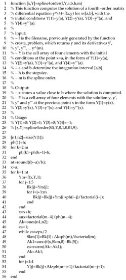
Figure 1. MATLAB code for computing approximate solutions of the problem in Equation (4) by means of m-th order splines.

The memory requirements for this function are $(m+12)$ matrices, i.e., m matrices for the cell-array variable ym, five matrices for the cell array variable $B_k$, three matrices for the variables Ak, Ak1, and Skm, furthermore, four matrices for the cell-array variable y.

Figure 2 reproduces the MATLAB code of the function create_problem, which automatically generates an output file, such as the one shown in Figure 3, containing all symbolical derivatives required for the main program, viz. Figure 1. The symbolical results in this file are then readily accessible as a function for computing the spline approximation with function spline4order. Note that for the computer algebra, the MATLAB interface to MuPAD is called [21,22]. All the essential codes, including future developments, will be made available for public use [23].

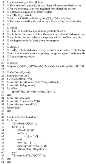
Figure 2. MATLAB function create_problem for automatically generating all symbolical derivatives required by the main code in Figure 1.

Figure 3. MATLAB function f.m generated by the code of Figure 2 for the problem given in Equation (31), using $m=9$ for the highest spline order. All relevant analytical derivatives have been set up automatically.

4. Numerical Examples

4.1. A Scalar Test Problem

As a starting point, we consider the problem of type Equation (4) for $Y\left(x\right)\in {\mathbb{C}}^{r\times q}$ with $r=q=1$, and apply our proposed method to the following scalar problem:

$$\left.\begin{array}{cccccc}\hfill & y^{\left(4\right)}\left(x\right)& =\hfill & \left(x^4-6x^2+3\right)y\left(x\right)& \hfill & \\ \\ \hfill y\left(0\right)& =& 1,\hfill & y^{\prime }\left(0\right)& \hfill =& 0\\ \\ \hfill y^{″}\left(0\right)& =& -1,\hfill & y^{‴}\left(0\right)& \hfill =& 0\end{array}\right\},0\le x\le 1.$$

(30)

This is a simple test problem and is recognized as an ideal benchmark test in the literature [9]. Its exact solution is known as $y\left(x\right)=e^{-x^2/2}$.

Since ${max}_{x\in [0,1]}\left\{x^4-6x^2+3\right\}=3$, we have a Lipschitz constant given by $L=3$. For splines of the seventh order ($m=7$), according to Theorem 1, we have $h<4.09062$ and take $n=10$ partitions with stepsize $h=0.1$. Computer algebra systems are most suitable to algebraically solve the equations arising from the algorithm. In this case, we employ Mathematica. All analytical results for the approximate splines are recorded in Table 1.

Table 1. Spline approximations for the scalar problem given in Equation (30).

Interval	Spline Approximations
$[0,0.1]$	$1-0.5x^2+0.125x^4-0.0208333x^6+0.000519274x^7$
$[0.1,0.2]$	$1+1.05916\times {10}^{-8}x-0.5x^2+3.47838\times {10}^{-6}{x}^3+0.124965x^4+0.000244182x^5-0.0218871x^6+0.00253921x^7$
$[0.2,0.3]$	$1+4.48369\times {10}^{-7}x-0.500007x^2+0.0000645975x^3+0.124627x^4+0.00138989x^5-0.0240704x^6+0.00433397x^7$
$[0.3,0.4]$	$1+4.84951\times {10}^{-6}x-0.500054x^2+0.000344851x^3+0.123613x^4+0.00360634x^5-0.0267723x^6+0.00574896x^7$
$[0.4,0.5]$	$1.00004-0.000641764x-0.495489x^2-0.0174827x^3+0.165188x^4-0.054248x^5+0.0176658x^6-0.00876821x^7$
$[0.5,0.6]$	$0.999995+0.0000593981x-0.500383x^2+0.00157178x^3+0.120685x^4+0.00792015x^5-0.0303493x^6+0.00703515x^7$
$[0.6,0.7]$	$1-1.66127\times {10}^{-6}x-0.500075x^2+0.000708329x^3+0.122137x^4+0.00645505x^5-0.0295281x^6+0.00683787x^7$
$[0.7,0.8]$	$1.00005-0.000496956x-0.497896x^2-0.0046218x^3+0.129965x^4-0.000447737x^5-0.0261447x^6+0.0061268x^7$
$[0.8,0.9]$	$1.00024-0.00225309x-0.491134x^2-0.0190941x^3+0.148561x^4-0.0147911x^5-0.0199957x^6+0.00499666x^7$
$[0.9,1.0]$	$1.00081-0.00677476x-0.475679x^2-0.0484533x^3+0.182039x^4-0.0377048x^5-0.0112802x^6+0.00357551x^7$

In Table 2, we specify the difference between the estimates of our numerical approach and the exact solution. The maximums of these errors are indicated for each subinterval. Obviously, the error for each subinterval is lower than the predicted global error of $O\left({10}^{-6}\right)$, but each local error is necessarily increasing while iterating from the first to the last subinterval.

Table 2. Approximation errors for the scalar problem given in Equation (30).

Interval	$[0,0.1]$	$[0.1,0.2]$	$[0.2,0.3]$	$[0.3,0.4]$	$[0.4,0.5]$
Max. error	$2.59117\times {10}^{-11}$	$9.30152\times {10}^{-10}$	$5.54498\times {10}^{-9}$	$1.85921\times {10}^{-8}$	$4.83612\times {10}^{-8}$
Interval	$[0.5,0.6]$	$[0.6,0.7]$	$[0.7,0.8]$	$[0.8,0.9]$	$[0.9,1.0]$
Max. error	$1.48407\times {10}^{-7}$	$4.29331\times {10}^{-7}$	$1.00674\times {10}^{-6}$	$1.99556\times {10}^{-6}$	$3.50949\times {10}^{-6}$

4.2. A Nonlinear Scalar Test Problem

This problem appears in Refs. [24] (p. 1003), [25], although for different intervals of the form $[0,b]$:

$$y^{\left(4\right)}\left(x\right)=y^2\left(x\right)+{cos}^2\left(x\right)+sin\left(x\right)-1,0<x\le b,$$

(31)

$$y\left(0\right)=0,y^{\prime }\left(0\right)=1,y^{″}\left(0\right)=0,y^{‴}\left(0\right)=-1.$$

Its exact solution is $y\left(x\right)=sin\left(x\right)$.

Note that for this particular test problem, the usage example in Figure 2 shows how to automatically produce the corresponding derivatives in the form of a MATLAB function f.m as required by the function spline4order. The output is shown in Figure 3. Afterwards, the execution of the usage example in Figure 1 computes all spline approximations for this test.

Figure 4 displays four graphics for the relative errors at $b=1$, taking as stepsizes $h={10}^{-1}$, $h={10}^{-2}$, $h={10}^{-3}$ and $h={10}^{-4}$, by also varying spline order m. In general, the error committed decreases by increasing the spline order. Similarly, the error generally reduces as we decrease the stepsize. However, for $m=10$, the error acquired for $h={10}^{-3}$ is less than the error for $h={10}^{-4}$. This is due to the increase in the number of floating point operations. Table 3 lists the corresponding relative errors.

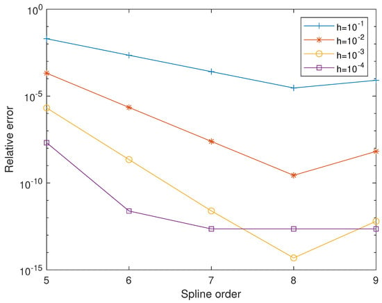
Figure 4. Relative errors at $b=1$ for the problem given in Equation (31), for several stepsizes ($h={10}^{-1},{10}^{-2},{10}^{-3},{10}^{-4}$), and varying spline orders ($m=5,6,7,8,9$).

Table 3. Relative errors at $b=1$ for the problem given in Equation (31) with varying spline orders m and stepsizes h.

m	5	6	7	8	9
$h={10}^{-1}$	$1.99\times {10}^{-2}$	$2.24\times {10}^{-3}$	$2.55\times {10}^{-4}$	$2.93\times {10}^{-5}$	$8.09\times {10}^{-5}$
$h={10}^{-2}$	$2.08\times {10}^{-4}$	$2.23\times {10}^{-6}$	$2.47\times {10}^{-8}$	$2.76\times {10}^{-10}$	$6.57\times {10}^{-9}$
$h={10}^{-3}$	$2.08\times {10}^{-6}$	$2.22\times {10}^{-9}$	$2.48\times {10}^{-12}$	$4.88\times {10}^{-15}$	$6.27\times {10}^{-13}$
$h={10}^{-4}$	$2.08\times {10}^{-8}$	$2.44\times {10}^{-12}$	$2.27\times {10}^{-13}$	$2.28\times {10}^{-13}$	$2.27\times {10}^{-13}$

Figure 5 provides five graphics with the relative errors for spline orders $m=5,6,7,8$, and 9, varying the final point of the interval ($b=1,2,3,4$, and 5). A fixed stepsize $h={10}^{-3}$ is considered. Obviously, the error increases as the value b grows. Similarly, the error improves when the stepsize decreases. Clearly, the highest precision is obtained for $m=8$.

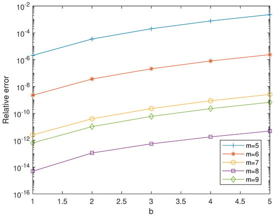
Figure 5. Relative errors for the problem given in Equation (31), for several spline orders ($m=5,6,7,8,9$). We discretely vary the value for $b=1,2,3,4$, and 5, with a fixed stepsize $h={10}^{-3}$.

4.3. A Matrix Differential Equation

The next example focuses on a type of matrix problem involving complex square matrices $Y\left(t\right)\in {\mathbb{C}}^{r\times r}$, satisfying the general differential equation

$$Y^{\left(4\right)}\left(t\right)+P\left(t\right)Y^{‴}\left(t\right)+Q\left(t\right)Y^{″}\left(t\right)+R\left(t\right)Y^{\prime }\left(t\right)+S\left(t\right)Y\left(t\right)=0,$$

(32)

where $P\left(t\right),Q\left(t\right),R\left(t\right)$ and $S\left(t\right)$ are continuous ${\mathbb{C}}^{r\times r}$-valued functions on an interval $J\subset \mathbb{R}$. Later on, we will choose these functions to be compatible with Equation (4).

In agreement with Ref. [26], we introduce the concept of a fundamental set of solutions for Equation (32). Its definition is as follows:

Definition 1.

Consider Equation (32). We say that a set of solutions $\{Y_1,Y_2,Y_3,Y_4\}$ is a fundamental set of solutions of Equation (32); in the interval J, if any solution Z of Equation (32) defined in J, the matrices $A,B,C,D\in {\mathbb{C}}^{r\times r}$ exist, uniquely determined by Z, such that

$$Z\left(t\right)=Y_1\left(t\right)A+Y_2\left(t\right)B+Y_3\left(t\right)C+Y_4\left(t\right)D,t\in J.$$

(33)

The following result provides a useful characterization of a fundamental set of solutions for Equation (32), and it may be regarded as a matrix analogue of Liouville’s formula for the scalar case [26].

Lemma 1.

Let $\{Y_1,Y_2,Y_3,Y_4\}$ be a set of solutions of Equation (32) defined on the interval J of the real line, and let $W\left(t\right)$ be the block matrix function

$$W\left(t\right)=\left(\begin{array}{cccc}{Y}_1\left(t\right)& Y_2\left(t\right)& Y_3\left(t\right)& Y_4\left(t\right)\\ Y_1^{\prime }\left(t\right)& Y_2^{\prime }\left(t\right)& Y_3^{\prime }\left(t\right)& Y_4^{\prime }\left(t\right)\\ Y_1^{″}\left(t\right)& Y_2^{″}\left(t\right)& Y_3^{″}\left(t\right)& Y_4^{″}\left(t\right)\\ Y_1^{‴}\left(t\right)& Y_2^{‴}\left(t\right)& Y_3^{‴}\left(t\right)& Y_4^{‴}\left(t\right)\end{array}\right)\in {\mathbb{C}}^{4r\times 4r}.$$

(34)

Then, the set $\{Y_1,Y_2,Y_3,Y_4\}$ is a fundamental set solutions of Equation (34) on J if there exists a point $t_1\in J$, such that $W\left(t_1\right)$ is non-singular in ${\mathbb{C}}^{4r\times 4r}$. In this case, $W\left(t\right)$ is non-singular for all $t\in J$.

Proof of Lemma 1.

Since $\{Y_1,Y_2,Y_3,Y_4\}$ are solutions of Equation (32), it follows that $W\left(t\right)$ defined by Equation (34) satisfies

$$W^{\prime }\left(t\right)=\left(\begin{array}{cccc}0& I& 0& 0\\ 0& 0& I& 0\\ 0& 0& 0& I\\ -S\left(t\right)& -R\left(t\right)& -Q\left(t\right)& -P\left(t\right)\end{array}\right)W\left(t\right),t\in J,$$

(35)

where I denotes the identity matrix of ${\mathbb{C}}^{r\times r}$. Thus, if $G(t,s)$ is the transition-state matrix of Equation (35), such that $G(t,t)=I$, see [27] (p. 598), it follows that $W\left(t\right)=G(t,t_1)W\left(t_1\right)$ for all $t\in J$. Hence, the result is established because $G(t,s)$ is invertible for all $t,s\in J$.    □

Returning to our specific matrix problem at hand, we consider for our test case an invertible matrix $A\in {\mathbb{C}}^{r\times r}$ and the differential equation

$$Y^{\left(4\right)}\left(x\right)-A^{4}Y\left(x\right)=0,0\le x\le 1,$$

(36)

where $Y\left(x\right)\in {\mathbb{C}}^{r\times r}$. This equation is a special case of Equation (32) with $P\left(t\right)=Q\left(t\right)=R\left(t\right)=0$ and $S\left(t\right)=A^4$. Thus, all coefficients are continuous ${\mathbb{C}}^{r\times r}$-valued functions on interval $[0,1]$. For the solutions, it is easy to check that the matrix functions

$$\left\{X_1\left(x\right)=e^{(-Ax)},X_2\left(x\right)=e^{\left(Ax\right)},X_3\left(x\right)=cos\left(Ax\right),X_4\left(x\right)=sin\left(Ax\right)\right\}$$

satisfy Equation (36). To show that this set is also a fundamental set of solutions of Equation (36), we will use Lemma 1. In this case, one obtains

$$\begin{array}{ccc}\hfill W\left(x\right)& =& \left(\begin{array}{cccc}{X}_1\left(x\right)& X_2\left(x\right)& X_3\left(x\right)& X_4\left(x\right)\\ X_1^{\prime }\left(x\right)& X_2^{\prime }\left(x\right)& X_3^{\prime }\left(x\right)& X_4^{\prime }\left(x\right)\\ X_1^{″}\left(x\right)& X_2^{″}\left(x\right)& X_3^{″}\left(x\right)& X_4^{″}\left(x\right)\\ X_1^{‴}\left(x\right)& X_2^{‴}\left(x\right)& X_3^{‴}\left(x\right)& X_4^{‴}\left(x\right)\end{array}\right)\hfill \\ & =& \left(\begin{array}{cccc}{e}^{(-Ax)}& e^{\left(Ax\right)}& cos\left(Ax\right)& sin\left(Ax\right)\\ -A{e}^{(-Ax)}& A{e}^{\left(Ax\right)}& -Asin\left(Ax\right)& Acos\left(Ax\right)\\ A^2{e}^{(-Ax)}& A^2{e}^{\left(Ax\right)}& -A^{2}cos\left(Ax\right)& -A^{2}sin\left(Ax\right)\\ -A^3{e}^{(-Ax)}& A^3{e}^{\left(Ax\right)}& A^{3}sin\left(Ax\right)& -A^{3}cos\left(Ax\right)\end{array}\right),\hfill \end{array}$$

and still needs to confirm that $W\left(x_0\right)$ is non-singular for some value $x_0\in [0,1]$. To show this, we consider $x_0=0$ and the matrix block $W\left(0\right)=M$ such that

$$M=\left(\begin{array}{cccc}I& I& I& 0\\ -A& A& 0& A\\ A^2& A^2& -A^2& 0\\ -A^3& A^3& 0& -A^3\end{array}\right),$$

where I denotes the identity matrix of ${\mathbb{C}}^{r\times r}$, and whose determinant $\left|M\right|$ is exactly $|W\left(0\right)|$. It is straightforward to verify that

$$\underset{N}{\underbrace{\left(\begin{array}{cccc}I& 0& 0& 0\\ 0& I& 0& 0\\ -A^2& 0& I& 0\\ 0& -A^2& 0& I\end{array}\right)}}M=\underset{S}{\underbrace{\left(\begin{array}{cccc}I& I& I& 0\\ -A& A& 0& A\\ 0& 0& -2A^2& 0\\ 0& 0& 0& -2A^3\end{array}\right)}},$$

(37)

where the block matrices N and S are invertible, with results

$$\begin{array}{ccccccc}\hfill N^{-1}& =& \left(\begin{array}{cccc}I& 0& 0& 0\\ 0& I& 0& 0\\ A^2& 0& I& 0\\ 0& A^2& 0& I\end{array}\right)\hfill & ,& S^{-1}& \hfill =& \frac{1}{4}\left(\begin{array}{cccc}2I& -2A^{-1}& A^{-2}& -A^{-3}\\ 2I& 2A^{-1}& A^{-2}& A^{-3}\\ 0& 0& -2A^{-2}& 0\\ 0& 0& 0& -2A^{-3}\end{array}\right).\end{array}$$

Next, taking the determinants on both sides of Equation (37), one concludes that $\left|M\right|\ne 0$, and thus, $W\left(x\right)$ is non-singular by Lemma 1. Furthermore, the set

$$\left\{X_1\left(x\right)=e^{(-Ax)},X_2\left(x\right)=e^{\left(Ax\right)},X_3\left(x\right)=cos\left(Ax\right),X_4\left(x\right)=sin\left(Ax\right)\right\}$$

is a fundamental set of solutions for Equation (36).

To carry out the numerics, we now select the initial value problem

$$\left.\begin{array}{cccccc}\hfill & Y^{\left(4\right)}\left(x\right)\hfill & =\hfill & A^{4}Y\left(x\right)& \hfill & \\ \\ Y\left(0\right)\hfill & =\hfill & I,\hfill & Y^{\prime }\left(0\right)& \hfill =& 0\\ \\ Y^{″}\left(0\right)\hfill & =\hfill & -A^2,\hfill & Y^{‴}\left(0\right)& \hfill =& 0\end{array}\right\},0\le x\le 1,$$

(38)

which has the unique and exact solution $Y\left(x\right)=cos\left(Ax\right)$. We choose $A=\left(\begin{array}{cc}1& 1\\ 0& 1\end{array}\right)$. Thus, the exact solution of Equation (38) is $cos\left(Ax\right)=\left(\begin{array}{cc}cos\left(x\right)& -xsin\left(x\right)\\ 0& cos\left(x\right)\end{array}\right)$. In this case, $f(x,Y)=A^{4}Y$ in Equation (4), and the corresponding Lipschitz constant is $L=4.23607$.

For our example, we consider splines of the seventh order ($m=7$). Then, according to Theorem 1, we obtain the condition $h<3.75257$. Therefore, we choose $n=10$ partitions with stepsize $h=0.1$.

Table 4 shows the maximum of the difference between the numerical estimates of our approach and the exact solution by taking the Fröbenius norm of this difference for each subinterval. Figure 6 analyzes the relative errors for this problem with varying stepsizes $h=0.1,0.01$, and $0.001$. As can be seen, the spline approximation considerably improves with smaller stepsizes. Apparently, the relative errors accumulate with each new subinterval as it of course propagates from one to the next subinterval. However, the approximations are well below the expected global error of $O\left({10}^{-6}\right)$ for $h=0.1$. For $h=0.01$, the local error also remains nearly of the order $O\left({10}^{-12}\right)$. However, for $h=0.001$ and working in practice with double-precision arithmetic ($2^{-53}\approx 1.1102·{10}^{-16}$), the truncation and rounding errors lastly determine the error margins. Nevertheless, the observed error of approximately $O\left({10}^{-14}\right)$ is fully satisfactory in almost all relevant applications.

Table 4. Approximation error for the matrix problem presented in Equation (36), with stepsize $h=0.1$.

Interval	$[0,0.1]$	$[0.1,0.2]$	$[0.2,0.3]$	$[0.3,0.4]$	$[0.4,0.5]$
Max. error	$2.0135\times {10}^{-12}$	$7.2457\times {10}^{-11}$	$4.3608\times {10}^{-10}$	$1.4836\times {10}^{-9}$	$3.7673\times {10}^{-9}$
Interval	$[0.5,0.6]$	$[0.6,0.7]$	$[0.7,0.8]$	$[0.8,0.9]$	$[0.9,1.0]$
Max. error	$7.9945\times {10}^{-9}$	$1.5020\times {10}^{-8}$	$2.5835\times {10}^{-8}$	$4.1559\times {10}^{-8}$	$6.3425\times {10}^{-8}$

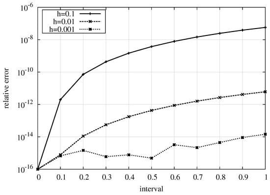
Figure 6. Relative errors for the matrix problem given in Equation (36), with seventh-order splines ($m=7$) and various stepsizes ($h=0.1,0.01$, and $0.001$).

4.4. A Nonlinear Matrix Problem

The following problem is similar to the Problem 4.7 from Ref. [14], but now applied to a fourth-order equation:

$$\left.\begin{array}{ccc}\hfill Y^{\left(4\right)}& =& Y^2\hfill \\ \hfill Y\left(0\right)& =& 0_n\hfill \\ \hfill Y^{\prime }\left(0\right)& =& {10}^{-2}{I}_n\hfill \\ \hfill Y^{″}\left(0\right)& =& {10}^{-3}{1}_n\hfill \\ \hfill Y^{‴}\left(0\right)& =& {10}^{-4}{1}_n\hfill \end{array}\right\},x\in [0,b],$$

(39)

where $0_n$, $I_n$ and $1_n$ are the null, the identity, and all-ones matrices of dimension n, respectively.

We have used the vpa function from the MATLAB Symbolic Math Toolbox for obtaining the “exact solution” with 256 digits of precision. All computations have IEEE double-precision arithmetic with unit round-off $u=2^{-53}\approx 1.11\times {10}^{-16}$. The “exact” solution is obtained whenever two consecutive spline orders (for fixed stepsize) present a relative error lower than the unit round-off for this accuracy.

Figure 7 shows four graphics of the relative errors at $b=2$ corresponding to the stepsizes $h=0.5$, $h=0.1$, $h=0.05$ and $h=0.01$, varying spline order m. As we can see, in general, the error committed becomes smaller and smaller with the increasing spline order. Similarly, the error gets smaller as we decrease the stepsize. However, for $m=9$, the error made for $h=0.05$ is less than the error made for $h=0.01$. Again, this is due to the resulting increase in the number of arithmetic operations. Table 5 gives the relative errors.

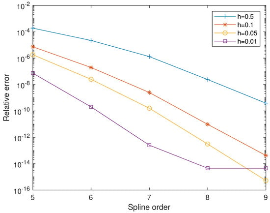
Figure 7. Relative errors at $b=2$ for the problem given in Equation (39), for various stepsizes ($h=0.5,0.1,0.05$, and $0.01$), varying the spline orders.

Table 5. Relative errors at $b=2$ for the problem given in Equation (39), for various stepsizes ($h=0.5,0.1,0.05$, and $0.01$), varying the spline orders.

m	5	6	7	8	9
$h=0.5$	$1.87\times {10}^{-4}$	$2.18\times {10}^{-5}$	$1.30\times {10}^{-6}$	$2.38\times {10}^{-8}$	$3.86\times {10}^{-10}$
$h=0.1$	$7.25\times {10}^{-6}$	$1.96\times {10}^{-7}$	$2.48\times {10}^{-9}$	$9.63\times {10}^{-12}$	$4.19\times {10}^{-14}$
$h=0.05$	$1.81\times {10}^{-6}$	$2.48\times {10}^{-8}$	$1.58\times {10}^{-10}$	$3.09\times {10}^{-13}$	$5.24\times {10}^{-16}$
$h=0.01$	$7.24\times {10}^{-8}$	$2.01\times {10}^{-10}$	$2.52\times {10}^{-13}$	$4.54\times {10}^{-15}$	$4.54\times {10}^{-15}$

The five graphics of Figure 8 correspond to the relative errors for the spline orders $m=5$, $m=6$, $m=7$, $m=8$ and $m=9$, varying the final points ($b=2,4,6,8,10$), for a fixed stepsize $h=0.05$. As can be seen, the error increases when the value of b grows. Similarly, the error drops as we decrease the stepsize. The most accurate results are obtained when $m=9$.

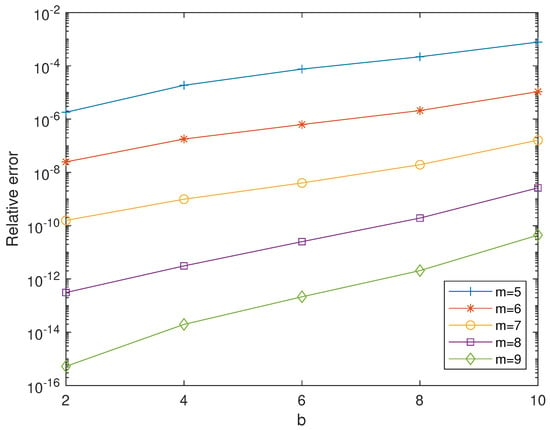
Figure 8. Relative errors for the problem given in Equation (39), for various spline orders ($m=5,6,7,8,9$), varying $b=2,4,6,8,10$ and with a fixed stepsize $h=0.05$.

5. Conclusions

This work describes a numerical procedure for solving fourth-order matrix differential equations of the type $Y^{\left(4\right)}\left(x\right)=f\left(x,Y\left(x\right)\right)$, where $Y\left(x\right)$ is a complex matrix—not necessarily a square matrix—and x is the parameter ranging over a real interval. In an iterative procedure, step by step, the solutions for all successive subintervals of the full interval are approximated in terms of matrix splines. This algorithm is straightforward to implement on a computer, consisting of the symbolical computation for the necessary derivatives and the subsequent numerical evaluation. The MATLAB code will be available to download [23].

Four standard benchmark tests, two scalar and two matrix cases, demonstrate that our numerical scheme produces spline approximations with suitable accuracy and is easy to implement. Moreover, with an appropriately chosen stepsize—provided by the theory and well adapted to the problem—an ever increasing improvement of the accuracy of the approximation can be reached up to the very limits of machine precision.

References

- Cantón, A.; Fernández-Jambrina, L. Interpolation of a spline developable surface between a curve and two rulings. Front. Inf. Technol. Electron. Eng. 2015, 16, 173–190. [Google Scholar] [CrossRef]
- Dokken, T.; Skytt, V.; Barrowclough, O. Trivariate spline representations for Computer Aided Design and Additive Manufacturing. Comput. Math. Appl. 2019, 78, 2168–2182. [Google Scholar] [CrossRef]
- Jator, S.N. Numerical integrators for fourth order initial and boundary value problems. Int. J. Pure Appl. Math. 2008, 47, 563–576. [Google Scholar]
- Bai, Z.; Wang, H. On positive solutions of some nonlinear fourth-order beam equations. J. Math. Anal. Appl. 2002, 270, 357–368. [Google Scholar] [CrossRef]
- Alomari, A.K.; Anakira, N.R.; Bataineh, A.S.; Hashim, I. Approximate solution of nonlinear system of BVP arising in fluid flow problem. Math. Probl. Eng. 2013, 2013, 7. [Google Scholar] [CrossRef]
- Malek, A.; Beidokhti, R.S. Numerical solution for high order differential equations using a hybrid neural network–optimization method. Appl. Math. Comput. 2006, 183, 260–271. [Google Scholar] [CrossRef]
- Boutayeb, A.; Chetouani, A. A mini-review of numerical methods for high-order problems. Int. J. Comput. Math. 2007, 84, 563–579. [Google Scholar] [CrossRef]
- Hussain, K.; Ismail, F.; Senu, N. Two Embedded Pairs of Runge-Kutta Type Methods for Direct Solution of Special Fourth-Order Ordinary Differential Equations. Math. Probl. Eng. 2015, 2015, 196595. [Google Scholar] [CrossRef]
- Famelis, I.; Tsitouras, C. On modifications of Runge–Kutta–Nyström methods for solving y(4) = f(x,y). Appl. Math. Comput. 2016, 273, 726–734. [Google Scholar] [CrossRef]
- Papakostas, S.; Tsitmidelis, S.; Tsitouras, C. Evolutionary generation of 7th order Runge–Kutta–Nyström type methods for solving y(4) = f(x,y). In Proceedings of the AIP Conference Proceedings 1702, Athens, Greece, 20–23 March 2015; AIP Publishing LLC: Melville, NY, USA, 2015; p. 190018. [Google Scholar]
- Olabode, B.T.; Omole Ezekiel, O. Implicit Hybrid Block Numerov-Type Method for the Direct Solution of Fourth-Order Ordinary Differential Equations. Am. J. Comput. Appl. Math. 2015, 5, 129–139. [Google Scholar]
- Adeyeye, O.; Omar, Z. Solving fourth order linear initial and boundary value problems using an implicit block method. In Proceedings of the Third International Conference on Computing, Mathematics and Statistics (iCMS2017), Langkawi, Malaysia, 5 November 2019; Springer Nature: Singapore, 2019; pp. 167–177. [Google Scholar]
- Defez, E.; Tung, M.M.; Ibáñez, J.; Sastre, J. Approximating a Special Class of Linear Fourth-Order Ordinary Differential Problems. In Proceedings of the European Consortium for Mathematics in Industry, Santiago de Compostela, Spain, 13–17 June 2016; Springer: Cham, Switzerland, 2016; pp. 577–584. [Google Scholar]
- Defez, E.; Ibáñez, J.; Alonso, J.M.; Tung, M.M.; Real-Herráiz, T. On the approximated solution of a special type of nonlinear third-order matrix ordinary differential problem. Mathematics 2021, 9, 2262. [Google Scholar] [CrossRef]
- Defez, E.; Tung, M.M.; Ibáñez, J.; Sastre, J. Approximating and computing nonlinear matrix differential models. Math. Comput. Model. 2012, 55, 2012–2022. [Google Scholar] [CrossRef]
- Defez, E.; Tung, M.M.; Solis, F.J.; Ibáñez, J. Numerical approximations of second-order matrix differential equations using higher degree splines. Linear Multilinear Algebra 2015, 63, 472–489. [Google Scholar] [CrossRef][Green Version]
- Graham, A. Kronecker Products and Matrix Calculus with Applications; John Wiley & Sons: New York, NY, USA, 1981. [Google Scholar]
- MATLAB, Version 9.12.0 (R2022a); The MathWorks Inc.: Natick, MA, USA, 2022.
- Flett, T.M. Differential Analysis; Cambridge University Press: Cambridge, MA, USA, 1980. [Google Scholar]
- Loscalzo, F.R.; Talbot, T.D. Spline function approximations for solutions of ordinary differential equations. SIAM J. Numer. Anal. 1967, 4, 433–445. [Google Scholar] [CrossRef]
- Fuchssteiner, B. (Ed.) MuPad Multi Processing Algebra Data Tool: Tutorial, MuPad Version 1.2; Springer: Basel, Switzerland, 1994. [Google Scholar]
- MATLAB. Symbolic Math in MATLAB. 2022. Available online: https://www.mathworks.com/discovery/mupad.html (accessed on 25 June 2022).
- Group of High Performance Scientific Computing (HiPerSC); Universitat Politècnica de València. MATLAB Code for Solving Non-Linear Matrix-Differential Equations. 2022. Available online: http://personales.upv.es/joalab/software/spline4order.zip (accessed on 25 June 2022).
- Jikantoro, Y.; Ismail, F.; Senu, N.; Ibrahim, Z. A class of hybrid methods for direct integration of fourth-order ordinary differential equations. Bull. Malays. Math. Sci. Soc. 2018, 41, 985–1010. [Google Scholar] [CrossRef]
- Hussain, K.; Ismail, F.; Senu, N. Solving directly special fourth-order ordinary differential equations using Runge–Kutta type method. J. Comput. Appl. Math. 2016, 306, 179–199. [Google Scholar] [CrossRef]
- Jódar, L. Explicit solutions for second order operator differential equations with two boundary value conditions. Linear Algebra Appl. 1988, 103, 73–86. [Google Scholar] [CrossRef]
- Kailath, T. Linear Systems; Prentice-Hall: Englewood Cliffs, NJ, USA, 1980; Volume 156. [Google Scholar]
Publisher’s Note: MDPI stays neutral with regard to jurisdictional claims in published maps and institutional affiliations. |
© 2022 by the authors. Licensee MDPI, Basel, Switzerland. This article is an open access article distributed under the terms and conditions of the Creative Commons Attribution (CC BY) license (https://creativecommons.org/licenses/by/4.0/).