A Priori Determining the Performance of the Customized Naïve Associative Classifier for Business Data Classification Based on Data Complexity Measures

Abstract

In the supervised classification area, the algorithm selection problem (ASP) refers to determining the a priori performance of a given classifier in some specific problem, as well as the finding of which is the most suitable classifier for some tasks. Recently, this topic has attracted the attention of international research groups because a very promising vein of research has emerged: the application of some measures of data complexity in the pattern classification algorithms. This paper aims to analyze the response of the Customized Naïve Associative Classifier (CNAC) in data taken from the business area when some measures of data complexity are introduced. To perform this analysis, we used classification datasets from real-world related to business, 22 in total; then, we computed the value of nine measures of data complexity to compare the performance of the CNAC against other algorithms of the state of the art. A very important aspect of performing this task is the creation of an artificial dataset for meta-learning purposes, in which we considered the performance of CNAC, and then we trained a decision tree as meta learner. As shown, the CNAC classifier obtained the best results for 10 out of 22 datasets of the experimental study.

1. Introduction

Supervised classification is widely used in almost every area nowadays. Its application in medicine [1,2,3], agriculture [4,5,6], education [7,8,9,10], sports [11,12,13], and social behavior in business [14,15,16], among other areas [17,18,19], is indisputable. However, it is well known that there is no classifier having an overall superior performance to the remaining ones for all problems. This fact was demonstrated by the No Free Lunch theorem [20].

Due to such conditions, the research devoted to determining the a priori performance of a given classifier in some specific problem, as well as the adequate classifiers for some tasks (the algorithm selection problem, ASP), have gained attention in the scientific community, since 70’s [21]. Several investigations have been carried out to address such issues, and in this context, the meta-learning task arose [22].

Meta-learning is devoted to a priori determining the expected performance of a learning algorithm under some specific problem [23]; that is, meta-learning strategies learn about the learners’ performances. Such approach has been used for optimization [24,25], clustering [26,27], regression [28], and supervised classification [29,30].

Recently, the application of some measures of data complexity in the pattern classification algorithms has emerged as a very promising vein of research [31]. Many studies have applied data complexity metrics to implement this concept [32,33,34,35,36]. However, there is no such research for associative classifiers; in addition, no research considers simultaneously the presence of multiclass, mixed (numerical and categorical), and missing (incomplete) data.

The detection of the type of problems for which a classifier is suitable is related to a concept coined in the specialized scientific literature: competence domains [37]. Certain authors use data complexity measures to define the domains of competence of pattern classifiers [32,33,34,37]. A collateral consequence of the use of complexity measures is that it has implications for algorithm performance in difficult regions of the problem representation space [35].

We selected the recently proposed Customized Naïve Associative Classifier (CNAC) [38] for this research because it showed satisfactory behavior for business-related problems, in particular, to determine the satisfaction of clients in the touristic sector. This paper aims to analyze the response of the CNAC to data from the business area when some measures of data complexity are introduced. The main purpose of the research is to establish a meta learner able to determine the a priori performance of the CNAC over business-related data.

We used classification datasets related to business (22 in total). Then, we computed the value of nine measures of data complexity. We analyzed the performance of CNAC, as well as other well-known supervised classifiers (C4.5 [39], Nearest Neighbor [40], RIPPER [41], Multilayer Perceptron with Backpropagation [42], and Support Vector Machines [43]). Then, we created an artificial dataset for meta-learning purposes, in which we considered the performance of CNAC, and then we trained a decision tree as meta learner.

As a relevant result of the previous process, the meta learner allows defining the competence domain of the CNAC. This has the consequence that it is possible to know the degree to which the classes are separable and the operating ranges where the CNAC exhibits good (or bad) results. It is pertinent to emphasize the scientific novelty of the paper, which consists of the characterization of the competence domain of the CNAC. This characterization of the domain of competence of the CNAC is carried out by generating a meta-learner in the form of a tree, which is based on measures of data complexity.

The remaining of the paper is as follows: Section 2 offers some previous works for determining the domains of competence of classifiers within the meta-learning approach. Section 3 details the classifiers as well as the business datasets used, while Section 4 explains the experimental protocol used in the research. Section 5 and Section 6 present and discusses the results obtained. The results include the complexity measures applied to the datasets, the comparison of CNAC concerning state-of-the-art classifiers, the statistical analysis, and the meta-learning procedure for the a priori determining the performance of CNAC. The paper ends with the conclusions and some directions for future works.

2. Previous Works

In this section, we briefly review some of the existing works on Algorithm Selection Problems (Section 2.1) and some of the most widely used supervised classifiers (Section 2.2).

2.1. Algorithm Selection Problem

Determining which classification algorithm will be appropriate for a certain dataset is an open problem within the international scientific community. Experts sometimes use their knowledge of the inner workings of classification algorithms to answer this question. Algorithm selection problems (ASP) were first analyzed by Rice [21] back in 1976, who presented the first model for this purpose. For ASP, it is generally suggested to carry out a mapping of measurable characteristics (meta-characteristics) over the problems (datasets) and then contrast them with the performance of classification algorithms to build an algorithm recommendation system [44].

Several surveys have addressed the meta-learning problem [22,23,25]. In addition, researchers have studied the ability to predict classifiers’ performance by employing data complexity measures. Sanchez et al. [36] contrasted the performance of the k Nearest Neighbor classifier with respect to data complexity measures. In addition, for microarray data, Morán-Fernández et al. [45] established relations among data complexity measures and the accuracy of four classifiers (C4.5, Naïve Bayes, Nearest Neighbor, and Support Vector Machines). However, none of the mentioned papers provide any meta-learner able to determine the expected performance of the analyzed classifiers.

Bernadó-Mansilla and Ho [32] introduced the first approach to the concept of domains of competence for the XCS classifier. To do so, they computed data complexity measures and determined the lower and upper limits under which the XCS classifier will perform well. They used binary (two classes) datasets with no missing values in their experiments. With their approach, a meta-learner in the form of decision rules was obtained.

Luengo and Herrera also were pioneers in finding the domain of competence of supervised classifiers. They provide a set of rules for the a priori determination of the fuzzy hybrid genetic-based machine learning (FH-GBML) classifier [34]. They also analyzed the behavior of three Artificial Neural Networks [37], and then in 2015 [35], they gave a step forward and provided automatic rules of good and bad behavior for three classifiers (C4.5, Nearest Neighbor, and Support Vector Machines) by considering 12 data complexity measures. Unfortunately, these research studies were carried out by using only binary datasets.

Following a similar perspective, Flores et al. [33] proposed a mechanism to select the most promising semi-naïve Bayesian network classifiers for a particular dataset based on the values of some complexity measures. They use a multi-label approach to obtain a meta learner by using problem transformation strategies. They did not provide rules for behavior due to the nature of the Naïve Bayes base classifier used in the meta-learning.

Having a meta learner allows the users to a priori knowledge if a particular supervised classifier will perform good or bad. It is possible to use the existing results in the literature for classifiers such as C4.5, Naïve Bayes, Nearest Neighbor, and Support Vector Machines. However, to the best of our knowledge, no research has been conducted to determine the domain of competence of an associative classifier. We aim to address this issue for the recently introduced CNAC classifier [38]. We also want to provide a meta-learner able to be explainable in the form of a set of rules or a decision tree.

2.2. State-of-the-Art Classifiers

There are several algorithms for supervised classification. Among them, we selected and applied five state-of-the-art classifiers (C4.5 [39], Nearest Neighbor (NN) [40], Repeated Incremental Pruning with Error Reduction (RIPPER) [41], Multilayer Perceptron with Backpropagation (MLP) [42], and Support Vector Machines (SVM) [43]) to use in comparisons. In the following, we explain the function of the aforementioned classifiers.

The C4.5 is a decision tree proposed by Quinlan. C4.5 is a deterministic classifier that uses Information Theory to determine the best splits over the tree. For numerical attributes, C4.5 finds the best value to split into two branches, and for categorical values, it expands one branch for each categorical value in the corresponding data. Missing numerical values are not considered in the induction of the tree, and missed categorical values are usually treated as another feature value [39].

The Nearest Neighbor classifier was introduced in the early 1960s [40], and it has remained one of the most used, well-performed supervised classifiers. It stores the training data and uses the notion of distance to classify instances. It is founded on the idea that similar instances will have the same class. For dealing with mixed and missing data, several dissimilarity functions have been proposed [46].

Repeated Incremental Pruning with Error Reduction (RIPPER) [41] is a rule-based classifier able to deal with mixed and incomplete data. During rule induction, RIPPER undergoes a process of obtaining the rules and pruning them. At the end of the training, a final set of rules is obtained. To classify a new instance, the first rule that is fulfilled will return the class label.

Multilayer Perceptron (MLP) is a Neural Network classifier consisting of several Perceptron-like units arranged in several layers [42]. The training of MLP is usually performed by the Backpropagation algorithm, which updates the weights of the connection between the neurons until some stop criterion is met. Once the MLP is trained, the instance to classify is presented to the input layer, and then it travels through the network to the output layer, in which the class label is returned.

Support Vector Machines (SVM) are based on the idea of obtaining a new representation space for the data, in which classes can be separated correctly [43]. The obtention of such space is computed using a mathematical function named kernel, responsible for data transformation and augmentation. To adjust the separation of the classes in the new space, some optimization procedures are used, typically the Sequential Minimal Optimization (SMO) algorithm. Once the SVM is trained to classify the new instance, it transforms it into the new representation space, and then the corresponding class label is obtained.

3. Materials, Methods, and Experimental Setup

We focused our research on the CNAC, which was introduced to deal with people’s attitudes related to business classification problems. Section 3.1 explains the CNAC classifier and details its functioning. The datasets used in the experiments are summarized in Section 3.2, and the experimental setup is explained in Section 3.3.

3.1. The Customized Naïve Associative Classifier

The Customized Naïve Associative Classifier (CNAC) is based on the NAC classifier [38]. The main modification is to substitute the MIDSO operator of NAC with a customized similarity operator. By that, it preserved the nature of NAC, and it is making it more flexible and useful for specific problems.

Let x and y be two instances, described by a set of features $A=\left\{A_1, \cdots , A_m\right\}$. The set of attributes A may have an associated set of attribute weights $W=\left\{w_1, \cdots , w_m\right\}$. We define a similarity function between two instances $sim\left(x,y, W\right)$ as a function that receives two instances and an optional set of feature weights and returns a real number in a way such that more akin instances have high similarity values, and very different instances have small similarity values.

Several dissimilarities have been proposed to handle hybrid and incomplete data. Usually, a dissimilarity $\mathrm{diss}$ is converted into a similarity function $sim$ as $sim=1/diss$. By using $sim\left(x,y, W\right)$ instead of MIDSO as an algorithm parameter, we can customize the classifier by maintaining the NAC advantages.

The CNAC maintains the advantages of the NAC classifier: it is able to deal with hybrid, incomplete and multiclass data; it has tractable computational complexity ($O\left(1\right)$ for training and $O\left(n\times m\right)$ for classification), where $n$ is the number of instances in the dataset, and it is an explainable classifier. In addition, it solves the main disadvantage of NAC, which is the use of a predefined similarity function.

The pseudocode of the CNAC is shown in Figure 1.

3.2. Datasets Used

We selected 22 datasets of such problems, including the clients’ responses to company offers, the employees’ probabilities of succeeding at work, and the people’s preferences towards clothes, among others. In the following, we briefly describe the selected datasets, which came from the Machine Learning Repository of the University of California at Irvine [47], and from the Kaggle site [48].

Table 1. Description of the used datasets.

Dataset	Instances	Attributes		Classes	Imbalance Ratio	Size (MB)
		Numeric	Categorical
alpha_bank	30,477	1	6	2	6.90	1.55
attribute_dataset	500 *	1	11	2	1.38	0.04
aug	19,158 *	2	10	2	3.01	1.71
bank_campaign	41,188 *	10	10	2	7.88	4.61
churn_modelling	10,000	6	4	2	3.91	0.45
behavior	400	2	1	2	1.80	0.01
segmentation	8068 *	3	6	4	1.22	0.33
targeting	6620	66	4	3	1.85	2.57
deposit2020	40,000	5	8	2	12.81	2.63
df_clean	358	3	16	2	9.23	0.04
employee_promo	54,808 *	5	7	2	10.74	3.09
employee_satisf	500	2	9	2	1.11	0.02
in-vehicle-coupon	12,684 *	1	24	2	1.32	2.07
marketing_camp	2240 *	14	13	2	5.71	0.21
marketing_series	6499 *	3	16	2	2.79	0.76
non-verbal-tourist	73 *	4	18	6	9.00	0.01
online_shoppers	12,330	10	7	2	5.46	1.10
promoted	24,016 *	4	2	5	5.44	0.50
telecom_churn	3333	10	0	2	5.90	0.13
telecom_churnV2	3333	15	4	2	5.90	0.27
telecust	1000	4	7	4	1.29	0.03
term_deposit	31,647	7	9	2	7.52	2.47

* Datasets having missing values.

present a summary of the description of the 22 used datasets, detailing the number of instances, numerical and categorical attributes, the presence of missing values (marked with an *), the number of classes, the imbalance ratio (IR) between the classes, and the size (in MB) of the corresponding dataset.

Regarding the size of the datasets, most of them are small (less than 2 MB), and the remaining are considered medium-sized (less than 5 MB). Of the selected datasets, 17 are imbalanced, with IR ranging from 1.80 to 10.74. The remaining five datasets are considered balanced, with IR from 1.11 to 1.38. As shown in Table 1, five of the compared datasets are multiclass, having three to six classes.

In the following, we describe the classification tasks related to the datasets.

Success of Bank Telemarketing Data (alpha_bank). A bank company wants to know the potential success of telemarketing campaigns (whether or not the client will subscribe to a long-term deposit). To select profitable potential subscribers, the bank considers the age, job, marital status, education, credit, as well as home and personal loans, among others [49].

Dress attributes (attribute_dataset). A shop needs to recommend dresses according to their characteristics, including style, price, rating, size, season, neckline, sleeve length, waistline, material, fabric type, decoration, and patterns, among others [50].

HR Analytics: Job Change of Data Scientists (aug). A company that is active in Big Data and Data Science wants to hire data scientists among people who successfully passed some courses that were conducted by the company [51].

Bank Marketing Campaign Subscriptions (bank_campaing). The dataset contains information about marketing campaigns that were conducted via phone calls from a Portuguese banking institution to their clients. The purpose of these campaigns is to prompt their clients to subscribe to a specific financial product of the bank (term deposit). After each call was conducted, the client had to inform the institution about their intention of either subscribing to the product (indicating a successful campaign) or not (unsuccessful campaign) [52].

Marketing Series: Customer Churn (churn_modelling). The dataset contains the details of the customers in a company. The columns are about its estimated salary, age, sex, etc., aiming to provide all details about a client. This dataset contains details of a bank’s customers, and the target variable is a binary variable reflecting the fact whether the customer left the bank (closed his account) or he/she continues to be a customer [53].

Predicting Profitable Customer Segments (targeting). Marketing is a key component of every modern business. Companies continuously re-invest large cuts of their profits for marketing purposes, trying to target groups of customers who have the potential to bring back the highest Return on Investment (ROI) for the company. The cost of marketing can be very high though, meaning that the decision about which customer group to target is of great financial importance. This dataset was made available by an online retail company that has collected historical data about such groups of customers, tracked the profitability of each group after the respective marketing campaign, and retrospectively assessed whether investing in marketing spending for that group was a good choice [54].

Customer Behavior (behavior). The data represent details about 400 clients of a company, including the unique ID, the gender, the age of the customer, and the salary. Besides this, it has information regarding the buying decision—whether the customer decided to buy specific products or not [55].

Customer Segmentation (segmentation). An automobile company has plans to enter new markets with their existing products (P1, P2, P3, P4, and P5). After intensive market research, they have deduced that the behavior of the new market is similar to their existing market. In their existing market, the sales team has classified all customers into four segments (A, B, C, and D). Then, they performed segmented outreach and communication for different segments of customers. This strategy has worked exceptionally well for them. They plan to use the same strategy in new markets and have identified 2627 new potential customers [56].

Deposit Subscription—What Makes Consumers Buy? (deposit2020). This dataset corresponds to customers who will (and will not) subscribe to long-term deposits in 2020. The objective is to predict the decision of the targeted audience and to focus the campaigns on the clients who will probably subscribe to the company [57].

Warranty Claims (df_clean). This dataset [58] corresponds to clients who filled warranty claims, and the objective is to determine if such claims are fraudulent or not. This is cleaned data from the previous (Warranty Claims Data set), available at [59].

HR Analysis Case Study (employee_promo). Every year, around 5% of the employees have been promoted in certain companies. This dataset includes the information to predict if an employee will be promoted or not [60].

Employee Satisfaction Index Dataset (employee_satisf). This is a fictional dataset created to help the data analysts play around with the trends and insights on the employee job satisfaction index [61].

In-vehicle coupon recommendation Data Set (in-vehicle-coupon). These data [62] were collected via a survey on Amazon Mechanical Turk. The survey describes different driving scenarios, including the destination, current time, weather, passenger, etc., and then asks the person whether he will accept the coupon if he is the driver. For more information about the dataset, please refer to [63].

Marketing Campaign (marketing_camp). The purpose of this dataset is to provide a significant boost to the efficiency of a marketing campaign by increasing responses or reducing expenses. The objective is to predict who will respond to an offer for a product or service [64].

Marketing Series: Customer Churn (marketing_series). This dataset contains data from a telecom company. The objective is to predict which customers will stop being customers (churn) and those that will remain customers and then take action accordingly [65].

Non-Verbal tourist (non-verbal-tourist). This dataset represents the non-verbal preferences of hotel guests in Jardines del Rey, Cuba. The objective is to predict the preferences of new guests and to classify them into one of the six groups of clients [38].

Purchasing intentions (online_shoppers). The dataset [66] consists of features belonging to 12,330 sessions. The dataset was formed so that each session would belong to a different user in one year to avoid any tendency to a specific campaign, special day, user profile, or period. The objective is to predict if the users will buy or not the products [67].

Promotion response and target datasets (promoted). The context of this business problem is a new product introduction. The organization is interested in building a model to select the best customers for contacting from the pool of customers not contacted. The promoted dataset provides response information along with profiles of customers who are contacted [68].

Customer Churn (telecom_churn). With the rapid development of the telecommunication industry, the service providers are inclined more towards the expansion of the subscriber base. To meet the need of surviving in the competitive environment, the retention of existing customers has become a huge challenge. It is stated that the cost of acquiring a new customer is far more than that of retaining the existing one. Therefore, the telecom industries must use advanced analytics to understand consumer behavior and, in turn, predict the association of the customers as to whether or not they will leave the company. This dataset contains customer-level information for a telecom company. Various attributes related to the services used are recorded for each customer [69].

Client churn rate in Telecom sector (telecom_churnV2). Orange Telecom’s Churn Dataset, which consists of cleaned customer activity data (features), along with a churn label specifying whether a customer canceled the subscription, will be used to develop predictive models [70].

Customer Classification (telecust). The dataset contains various information about their customers such as age and region, among others. It contains the information taken by a Telecommunication company. The objective is to predict the correct segment (type) of a customer [71].

Term Deposit Prediction Data Set (term_deposit). Term deposits are a major source of income for a bank. A term deposit is a cash investment held at a financial institution. The money is invested for an agreed rate of interest over a fixed amount of time or term. The bank has various outreach plans to sell term deposits to their customers, such as email marketing, advertisements, telephonic marketing, and digital marketing. Telephonic marketing campaigns remain one of the most effective ways to reach out to people. However, banks require huge investments, as large call centers are hired to execute these campaigns. Hence, it is crucial to identify the customers most likely to convert beforehand so that they can be specifically targeted via call [72].

3.3. Experimental Setup

First, we want to explore the influence of data complexity on the performance of the CNAC classifier. In particular, we aim to detect the conditions that made this classifier perform adequately and, therefore, establish rules to a priori known if it is convenient or not to apply this classifier to a certain problem. Figure 2 shows the diagram of the experiments for this aim.

Our experimental configuration started with the division of the datasets into training and testing by means of a five-fold cross-validation procedure. After that, we computed data complexity measures over the training sets. In addition, we trained and tested the supervised classifiers and computed their performance. After that, we carried out a statistical analysis of the results, considering the performance of CNAC and the remaining supervised classifiers.

To obtain a meta-learner, we constructed a meta-dataset using as meta-features the values of the data complexity measures and, as class labels, the qualitative performance obtained by CNAC. We trained a C4.5 classifier over the meta dataset, and we obtained a set of rules defining the a priori expected performance of CNAC.

We divided the datasets using five-fold cross-validation due to the imbalanced nature of the data and averaged the results. Then, we applied five state-of-the-art classifiers (C4.5 [39], Nearest Neighbor (NN) [40], Repeated Incremental Pruning with Error Reduction (RIPPER) [41], Multilayer Perceptron with Backpropagation (MLP) [42], and Support Vector Machines (SVM) [43]). Both the data partitioning and the classifier execution were made with the KEEL software [73], except for the NN classifier, in which we used the EPIC software to be able to use the same dissimilarity function as CNAC. KEEL software automatically inputs missing data if needed by the classification algorithm, and its internal codification converts categorical data to numerical. With such procedures, algorithms such as SVM and MLP can be executed.

In addition, we applied the CNAC classifier, but with no feature weighting, to obtain a baseline performance. This was made by using the EPIC software [74,75], in which the CNAC classifier is available. EPIC software does not make any data preprocessing by defaults, and due to CNAC can handle missing and incomplete data, it was executed without any data preprocessing.

In the execution of the algorithms, we used the default parameter values provided by KEEL and EPIC, except for NN and CNAC in the non-verbal-tourist data, where we used the dissimilarity function suggested by the authors of the dataset [38]. In addition, we set the dissimilarity for NN as the same as CNAC by using the EPIC software.

Table 2. Parameter of the compared classifiers.

Classifier	Parameters
C4.5	Pruned: true; Confidence: 0.25; Instances per leaf: 2
NN	K: 1; Dissimilarity: HEOM [46], except for the non-verbal-tourist data, in which we used the function suggested in [38]
RIPPER	K: 2; Grow pct: 0.66
MLP	Hidden layers: 2; Hidden nodes: 15; Transfer: hyperbolic tangent; Eta: 0.15; Alpha: 0.10; Lambda: 0.0; Test data: true; Validation data: false; Cross validation: false; Cycles: 10,000; Improve: 0.01; Typify inputs: true
SVM	Kernel: Radial Basis Function (RBF); C: 100; Eps: 0.001; Degree: 1; Gamma: 0.01; Coef0: 0.0; Nu: 0.1; p: 1.0; Shrinking: 1
CNAC	Dissimilarity: HEOM [46], except for the non-verbal-tourist data, in which we used the function suggested in [38]; Attribute weighting: None

shows the parameters of the classifiers

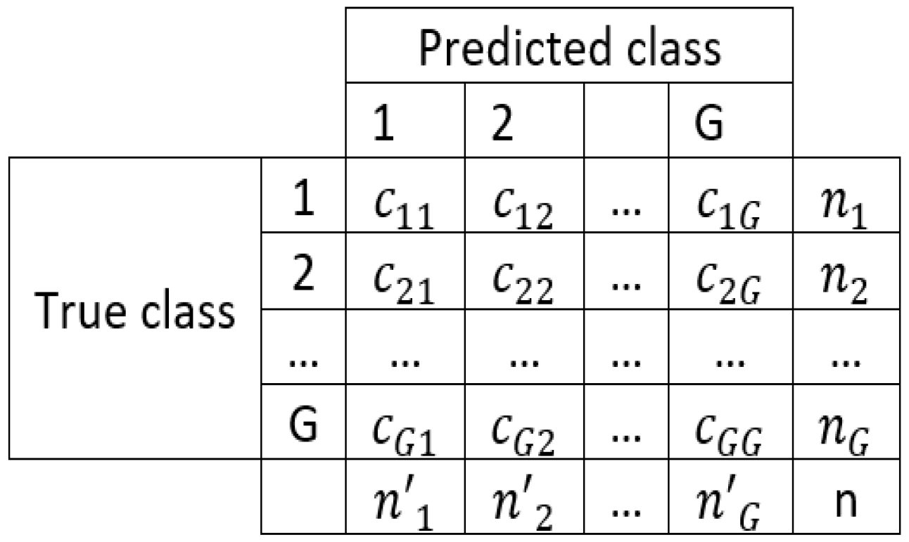
As a performance measure, we used the Non-Error Rate (NER), also known as averaged sensitivity [76]. Given a confusion matrix of G classes (Figure 3), the NER measure is computed as:

$$\mathrm{NER}=\frac{{\sum }_{g=1}^{G}S{n}_g}{\mathrm{G}}$$

(1)

where

$$S{n}_g=\frac{c_{gg}}{n_g}$$

(2)

NER is suitable for multiclass data, and it is robust for imbalanced data. We computed the NER values for the state-of-the-art classifiers by using the result files (real and assigned labels) provided by KEEL; for CNAC and NN, we just used the NER values provided by the EPIC software. Section 4.1 discusses the obtained results.

Then, we conducted the corresponding statistical analysis of performance (Section 4.2), comparing the CNAC with respect to the state-of-the-art classifiers by using the Friedman [77] and Holm [78] tests. According to the results obtained, we established the CNAC performance as Good, Regular, or Bad for each of the compared datasets.

In parallel, we evaluated nine complexity measures, the F1, F2, F3, N1, N2, N3, N4, T1, and T2 measures [31], which were computed using the KEEL software [73]. We did not include the measures L1, L2, and L3 because we have five multiclass datasets, and the KEEL implementation does not allow multiclass data for such measures. Section 4.3 discusses the results concerning data complexity.

Later, we created a new dataset for meta-learning purposes, having as condition attributes the complexity measures and as decision attribute the CNAC performance (Good, Regular, or Bad) for each of the compared datasets. Then, we trained a C4.5 decision tree to obtain the rules to a priori determine if the CNAC classifier is suitable for a certain classification problem. The corresponding results are in Section 4.4.

4. Results

4.1. Performance of the Classifiers

We executed the C4.5, NN, RIPPER, MLP, SVM, and CNAC classifies over the selected datasets, using the five-fold cross-validation procedure. We averaged the performance results obtained for each fold using the result files (real and assigned labels) provided by KEEL; for NN and CNAC, we just used the averaged NER values provided by the summary file returned by the EPIC software. In

Table 3. Performance of the compared classifiers according to averaged NER. The best results are highlighted in bold.

Dataset	C4.5	SVM	NN	MLP	RIPPER	CNAC
alpha_bank	0.50	0.51	0.52	0.53	0.56	0.84
attribute_dataset	0.51	0.46	0.51	0.50	0.49	0.48
aug	0.66	0.61	0.63	0.53	0.67	0.66
bank_campaign	0.75	0.67	0.72	0.61	0.70	0.87
churn_modelling	0.71	0.50	0.65	0.57	0.70	0.56
behavior	0.90	0.70	0.87	0.81	0.89	0.72
segmentation	0.50	0.50	0.42	0.35	0.48	0.42
targeting	0.45	0.38	0.41	0.38	0.48	0.45
deposit2020	0.70	0.51	0.62	0.53	0.63	0.85
df_clean	0.50	0.50	0.56	0.59	0.52	0.55
employee_promo	0.67	0.66	0.57	0.58	0.56	0.68
employee_satisf	0.47	0.50	0.52	0.50	0.47	0.53
in-vehicle-coupon	0.71	0.68	0.66	0.51	0.72	0.54
marketing_camp	0.61	0.54	0.61	0.50	0.71	0.66
marketing_series	0.68	0.65	0.42	0.69	0.71	0.72
non-verbal-tourist	0.47	0.33	0.61	0.25	0.54	0.73
online_shoppers	0.78	0.52	0.60	0.51	0.80	0.64
promoted	1.00	0.70	0.99	0.37	0.79	1.00
telecom_churn	0.81	0.55	0.73	0.57	0.83	0.65
telecom_churnV2	0.81	0.50	0.59	0.55	0.85	0.67
telecust	0.32	0.29	0.28	0.28	0.35	0.36
term_deposit	0.72	0.50	0.64	0.66	0.59	0.76
Times Best	5	0	1	1	7	10

, we report the NER values of the classifiers.

As shown in Table 3, the classifier with the best performance was CNAC. It obtained the best results in 10 datasets. RIPPER and C4.5 classifiers also obtained good performances, with seven and six wins, respectively. It is important to mention that several of the selected datasets are very complex, such as attribute_dataset, segmentation, targeting, df_clean, and telecust. In such datasets, the performances of the best classifiers were particularly low, at 0.51 (two classes), 0.50 (four classes), 0.48 (three classes), 0.59 (two classes), and 0.36 (four classes), respectively.

4.2. Statistical Analysis

For the statistical analysis, we used non-parametric tests. We set as null hypothesis H0 that there are no differences in the performance of the compared classifiers with respect to the Non-Error Rate (NER), and as alternative hypothesis H1 that there are differences in the performance of the compared classifiers with respect to the Non-Error Rate (NER). We set a significance value $\alpha =0.05$, for 95% of confidence.

We applied the Friedman test [77] and the Holm post hoc test [78], both suggested in [79], to determine if the differences found are significant or not. The Friedman test obtained a p-value of 0.0 (due to rounding), and therefore, we reject the null hypothesis.

Table 4. Ranking obtained by Friedman’s test.

Classifier	Ranking
CNAC	2.5227
RIPPER	2.6591
C4.5	2.6818
NN	3.5227
MLP	4.6818
SVM	4.9318

shows the ranking of the compared classifiers, according to the Friedman test.

As expected, the CNAC classifier is the first in the ranking, followed closely by RIPPER and C4.5.

Table 5. Results of Holm’s test.

i	Algorithm	z	p-Value	$\mathbf{Holm} \left(\mathit{\alpha }/\mathit{i}\right)$
5	SVM	4.270862	0.000019	0.010000
4	MLP	3.827659	0.000129	0.012500
3	NN	1.772811	0.076260	0.016667
2	C4.5	0.282038	0.777914	0.025000
1	RIPPER	0.241747	0.808976	0.050000

shows the results of Holm’s test.

Holm’s test rejects the null hypothesis for MLP and SVM classifiers with a 95% of confidence. That is, the test found significant differences between CNAC and both MLP and SVM, according to Non-Error Rate. The null hypothesis was not rejected for the RIPPER and C4.5 classifiers (both with high p-value). For the NN classifier, the p-value obtained was extremely low (0.076260), but not low enough to reject the null hypothesis. Therefore, further experiments are needed to establish the existence or not of significant differences in Non-Error Rate while comparing CNAC and NN over business datasets.

4.3. Complexity Measures for Meta-Learning

After obtaining the performance of the CNAC, we want to determine under what conditions it achieves good results. To do so, we compute data complexity measures. We summarize the description and reference of each complexity measure in

Table 6. Description of the data complexity measures.

Measure	Name	Based on	Proportion	Multiclass
F1	Maximum Fisher’s discriminant ratio	Features	Inverse	Yes
F2	The volume of the overlapping region	Features	Direct	Yes
F3	Maximum individual feature efficiency	Features	Inverse	Yes
L1	Sum of the Error Distance by Linear Programming	Linearity	Direct	No
L2	Error Rate of Linear Classifier	Linearity	Direct	No
L3	Non-Linearity of a Linear Classifier	Linearity	Direct	No
N1	Fraction of Borderline Points	Neighborhood	Direct	Yes
N2	The ratio of Intra/Extra Class Nearest Neighbor Distance	Neighborhood	Direct	Yes
N3	Error Rate of the Nearest Neighbor	Neighborhood	Direct	Yes
N4	Non-Linearity of the Nearest Neighbor Classifier	Neighborhood	Direct	Yes
T1	Fraction of Hyperspheres Covering Data	Topology	Direct	Yes
T2	Average Number of Features Per Dimension	Dimensionality	Direct	Yes

, as well as its value related to data complexity. We consider a direct proportion if higher values of the measure lead to higher data complexity and an inverse proportion otherwise. We also include if the measures support multiclass data.

We evaluated nine complexity measures, the F1, F2, F3, N1, N2, N3, N4, T1, and T2 measures [31], which were computed using the KEEL software [73]. We did not include the measures L1, L2, and L3 (also included in KEEL) because we have five multiclass datasets, and such measures do not support multiclass data.

In

Table 7. Values of the complexity measures in the datasets. The datasets with most complex values are in bold.

Dataset	F1	F2	F3	N1	N2	N3	N4	T1	T2
alpha_bank	0.01	$-\infty$	0.00	0.21	0.36	0.16	0.48	1.00	3483.09
attribute_dataset	0.02	0.22	0.01	0.69	1.01	0.51	0.35	1.00	33.33
aug	0.30	0.99	0.00	0.46	0.83	0.31	0.45	1.00	1277.20
bank_campaign	0.55	0.14	0.06	0.18	0.51	0.12	0.31	1.00	1647.52
churn_modelling	0.28	0.45	0.01	0.38	0.73	0.26	0.41	1.00	800.00
behavior	0.16	0.00	0.01	0.71	1.03	0.56	0.58	1.00	75.66
segmentation	1.34	0.64	0.20	0.32	0.24	0.21	0.24	0.80	106.67
targeting	0.26	1.00	0.00	0.72	1.00	0.57	0.60	0.99	717.16
deposit2020	0.93	0.16	0.00	0.14	0.35	0.10	0.36	0.99	2461.54
df_clean	0.38	0.41	0.11	0.24	0.35	0.18	0.45	1.00	15.07
employee_promo	0.34	0.46	0.00	0.17	0.65	0.11	0.44	1.00	3653.87
employee_satisf	0.02	1.00	0.00	0.71	1.03	0.54	0.45	1.00	36.36
in-vehicle-coupon	0.04	1.00	0.00	0.58	0.88	0.38	0.41	1.00	405.89
marketing_camp	0.24	0.00	0.03	0.30	0.53	0.20	0.44	1.00	66.37
marketing_series	0.62	0.48	0.00	0.39	0.75	0.27	0.32	0.99	273.64
non-verbal-tourist	$\infty$	$\infty$	0.84	0.67	1.14	0.47	0.40	0.99	2.65
online_shoppers	0.48	0.05	0.00	0.34	0.75	0.23	0.44	1.00	580.24
promoted	65.12	−0.47	1.00	0.14	0.32	0.07	0.06	0.97	3202.13
telecom_churn	0.18	0.35	0.01	0.34	0.66	0.23	0.46	1.00	266.64
telecom_churnV2	0.18	0.07	0.01	0.35	0.79	0.24	0.45	1.00	140.34
telecust	0.40	0.21	0.05	0.87	1.31	0.70	0.64	1.00	72.73
term_deposit	0.50	0.08	0.01	0.22	0.49	0.15	0.37	0.99	1582.35

, we present the results of the measures for the datasets. The results correspond to three feature-based measures (F1, F2, and F3), four neighborhood-based measures (N1, N2, N3, and N4), one network-based measure (T1), and one dimensionality-based measure (T2). We highlight the most complex problem for each measure in bold.

According to F1, which ranges from zero to infinity and has inverse proportion (higher values indicate simpler problems), the majority of the datasets have high complexity, with values lower than 1.50. Only the datasets non-verbal-tourist ($\infty$) and promoted (65.12) are considered simple. The F2 measure does not provide much information due to it ranges from $-\infty$ to $\infty$. Regarding F3 (also having inverse proportion and ranging from zero to one), the simplest problems are again non-verbal-tourist and promoted, and all remaining problems are considered complex, with values lower than 0.20.

For the neighborhood-based measures (N1, N2, N3, and N4), the hardest problem is telecust, and the simplest is promoted. All other datasets have variable complexity. The network-based measure T1 considers all datasets as complex, and therefore it does not allow us to differentiate among them. Last but not least, the dimensionality measure (T2) considers employee_promo as the hardest dataset. This is due to the number of attributes (12) and instances (54,808).

4.4. Meta-Learning

Having the data complexity measures, as well as the results of the performance of the CNAC, we constructed a dataset for meta-learning. Following the suggestions of [23], we used as condition attributes the nine complexity measures computed, and as decision attribute, the performance of the CNAC.

We divide the performance of CNAC into three groups: Good, Regular, and Bad. This measured the relative performance of CNAC as compared to other algorithms. The assignment of these three labels is necessarily empirical; the essence of this problem is similar to the essence of the kind of problems that led Zadeh to create fuzzy sets. For example, if we consider that an individual is “tall” when he measures 1.80 m and then we consider individuals with less height: 1.79 m, 1.78 m, 1.70 m, 1.69 m, and so on. At what point will we say that an individual was no longer labeled “high”? How tall does a human have to be to be “short”? Something similar happens with adjectives such as “big”, “medium”, and “small”. For example, be the question, is the Sun big? to which an astronomer would answer with another question: compared to what?

In the case at hand, there are clear cases that are easy to solve. For example, regardless of the dataset, if a classifier returns a balanced accuracy value of less than 0.5, that classifier is undoubtedly bad; on the other hand, if when testing a classifier on 10 datasets and it always returns 1 balanced accuracy, it would be absurd to say that this classifier is bad; on the contrary, we would say that it is good. The problem arises in the intermediate values between 0.5 and 1: what are the limits of values of the performance measures that lead us to decide if a classifier is Good, Regular, and Bad? The answer lies in common sense and in the comparison of the values that some of the known state-of-the-art classifiers throw on the same datasets. That is, in this research work, the labels Good, Regular, and Bad have been assigned, in a responsible manner, as a measure of the relative performance of CNAC as compared to other algorithms.

Considering the analysis, we selected as Regular the performances for three datasets (attribute_dataset, targeting, and df_clean); as Bad the performances for eight datasets (churn_modelling, behavior, segmentation, in-vehicle-coupon, marketing_camp, online_shoppers, telecom_churn, and telecom_churnV2); and as Good the performances for the remaining eleven datasets.

Then, we trained a C4.5 classifier and obtained the meta-learner classifier. Figure 4 shows the decision tree obtained. As shown, it only considers three attributes: the measures N1, N2, and T2, resulting in a pretty small tree (five leaves and size = 9).

The meta-learner obtained suggests that having a high number of instances and attributes is beneficial to the CNAC due to it tends to perform well in datasets with high T2. On the other hand, for smaller datasets, the neighborhood-based complexity measures intervene. The confusion matrix for the obtained meta learner is offered in Figure 5, and the detailed performance measures [76] for all classes are given in

Table 8. Detailed performance measure by class for the meta learner decision tree.

Measure	Good	Regular	Bad	Average
Sensitivity	0.909	0.667	1.000	0.859
Specificity	0.909	1.000	0.929	0.946
Precision	0.909	1.000	1.000	0.970
F1 score	0.909	0.800	1.000	0.903
Geometric Mean	0.909	0.816	0.964	0.896
Gini Index	0.818	0.667	0.929	0.804
Cosine	0.909	0.816	1.000	0.909

.

The results show that the class “Regular” is the one with less sensitivity and Gini Index, and therefore, further experiments are needed to correctly estimate the average performance of the CNAC.

5. Discussion

In this section, the results obtained in the previous section are discussed, and important aspects that emphasize the contribution of this paper to the state of the art are mentioned. First of all, it is pertinent to note that in Table 4, the CNAC classifier obtained the best results for ten datasets, while RIPER and C4.5 classifiers obtained the best results in six datasets. However, these data are not enough because it is required to determine if the differences in performance of the compared classifiers are significant or not; to elucidate it, we applied statistical tests.

Statistical tests yield remarkable results. For example, in Table 6, it is observed that the Holm test rejected the hypothesis having a p-value lower or equal to 0.016667 for a 95% of confidence. As shown, the Holm test did reject the hypothesis of the existence of significant differences in the performance of the CNAC with respect to the C4.5 and RIPPER classifiers and found CNAC to perform significantly better than MLP and SVM. For the NN classifier, the unadjusted p-value is 0.076260, which is close to the significance value $\alpha$; however, due to the adjustment made by the post hoc test, this result is not sufficient to reject the null hypothesis with a 95% of confidence.

Regarding the complexity measures for meta-learning, Table 8 shows the values of the complexity measures in the datasets. The complexity measures having direct proportions are interpreted by considering higher values lead to more complex problems. Inversely, the measures with inverse proportion (such as F3) are interpreted by considering that bigger values lead to less complex problems.

For dataset alpha-bank, the F2 measure obtained a minus infinity value; in addition, for the non-verbal tourist dataset, both F1 and F2 measures obtained infinity as a value. All remaining measures obtained adequate values for all datasets.

The inclusion of meta-learning processes means the culminating part of this research proposal. The results issued here are the most solid part of the most relevant scientific contributions. In this regard, it is pertinent to note that from the results of Table 8 we can conclude that CNAC is suitable for business datasets having $T2$ measure with values greater than 800, for datasets with $T2\le 36.36$ and $N2>1$, or for datasets having $T2>36.36$ and $N2>0.72$. For datasets with $T2>36.36$ and $N1\le 1,$ we do not recommend using CNAC.

Our experiments show that in the datasets in which CNAC had bad performance (churn_modelling, behavior, segmentation, in-vehicle-coupon, marketing_camp, online_shoppers, telecom_churn, and telecom_churnV2), the RIPPER and C4.5 classifiers tend to obtain good results. Therefore, although further research is needed to draw some conclusions, we can recommend using RIPPER or C4.5 classifiers in the scenarios in which CNAC is predicted to have poor behavior.

6. Conclusions and Future Works

In this article, we obtained as the main result a meta learner able to determine the a priori performance of the CNAC over business-related data. To achieve this purpose, we calculated nine measures of data complexity to the data of 22 datasets related to business, and we compared the performance of our proposal with some of the most important state-of-the-art classifiers. The first relevant conclusion is that, as illustrated in Table 4, the CNAC classifier obtained the best results for 10 datasets; in contrast, RIPER and C4.5 classifiers obtained the best results in six datasets.

The experimental design played a very important role in the success of our initial purpose. The experiments begin with the division of the datasets into training and testing by means of a five-fold cross-validation procedure. After that, the aforementioned calculation of the data complexity measures over the training sets was performed. After calculating the performance of our proposal and the state-of-the-art classifiers, we carried out a statistical analysis. The Friedman test and the Holm post hoc test allow us to establish that, indeed, there are significant differences between the performance of our proposal and the performance of the classifiers with which it is compared. The values obtained by Friedman’s test allow us to reject the null hypothesis, being the CNAC classifier the first in the ranking, followed closely by RIPPER and C4.5.

Additionally, it is necessary to emphasize that a very important aspect of performing this task is the creation of an artificial dataset for meta-learning purposes, in which we considered the performance of CNAC, and then we trained a decision tree as a meta-learner.

For future works, we want to corroborate the results of the meta-learner decision tree in other business-related datasets. In addition, we want to explore the influence of the similarity function in CNAC, as well as to investigate the possible inverse relation in performance between RIPPER, C4.5, and CNAC. We also want to explore the use of feature weighting in the performance of the CNAC.

References

1. Albahri, O.; Zaidan, A.; Albahri, A.; Zaidan, B.; Abdulkareem, K.H.; Al-Qaysi, Z.; Alamoodi, A.; Aleesa, A.; Chyad, M.; Alesa, R. Systematic review of artificial intelligence techniques in the detection and classification of COVID-19 medical images in terms of evaluation and benchmarking: Taxonomy analysis, challenges, future solutions and methodological aspects. J. Infect. Public Health 2020, 13, 1381–1396. [Google Scholar] [CrossRef] [PubMed]
2. Bria, A.; Marrocco, C.; Tortorella, F. Addressing class imbalance in deep learning for small lesion detection on medical images. Comput. Biol. Med. 2020, 120, 103735. [Google Scholar] [CrossRef] [PubMed]
3. Raj, R.J.S.; Shobana, S.J.; Pustokhina, I.V.; Pustokhin, D.A.; Gupta, D.; Shankar, K. Optimal feature selection-based medical image classification using deep learning model in internet of medical things. IEEE Access 2020, 8, 58006–58017. [Google Scholar] [CrossRef]
4. Deepa, N.; Ganesan, K. Hybrid rough fuzzy soft classifier based multi-class classification model for agriculture crop selection. Soft Comput. 2019, 23, 10793–10809. [Google Scholar] [CrossRef]
5. Li, Y.; Chao, X. ANN-based continual classification in agriculture. Agriculture 2020, 10, 178. [Google Scholar] [CrossRef]
6. Zheng, Y.-Y.; Kong, J.-L.; Jin, X.-B.; Wang, X.-Y.; Su, T.-L.; Zuo, M. CropDeep: The crop vision dataset for deep-learning-based classification and detection in precision agriculture. Sensors 2019, 19, 1058. [Google Scholar] [CrossRef] [Green Version]
7. Karthikeyan, V.G.; Thangaraj, P.; Karthik, S. Towards developing hybrid educational data mining model (HEDM) for efficient and accurate student performance evaluation. Soft Comput. 2020, 24, 18477–18487. [Google Scholar] [CrossRef]
8. Prada, M.A.; Domínguez, M.; Vicario, J.L.; Alves, P.A.V.; Barbu, M.; Podpora, M.; Spagnolini, U.; Pereira, M.J.V.; Vilanova, R. Educational data mining for tutoring support in higher education: A web-based tool case study in engineering degrees. IEEE Access 2020, 8, 212818–212836. [Google Scholar] [CrossRef]
9. Xu, W.; Hoang, V.T. MapReduce-Based Improved Random Forest Model for Massive Educational Data Processing and Classification. Mob. Netw. Appl. 2021, 26, 191–199. [Google Scholar] [CrossRef]
10. Zaffar, M.; Hashmani, M.A.; Savita, K.; Khan, S.A. A review on feature selection methods for improving the performance of classification in educational data mining. Int. J. Inf. Technol. Manag. 2021, 20, 110–131. [Google Scholar] [CrossRef]
11. Hsu, Y.-L.; Chang, H.-C.; Chiu, Y.-J. Wearable sport activity classification based on deep convolutional neural network. IEEE Access 2019, 7, 170199–170212. [Google Scholar] [CrossRef]
12. Lee, J.; Joo, H.; Lee, J.; Chee, Y. Automatic classification of squat posture using inertial sensors: Deep learning approach. Sensors 2020, 20, 361. [Google Scholar] [CrossRef] [PubMed] [Green Version]
13. Stöggl, T.; Holst, A.; Jonasson, A.; Andersson, E.; Wunsch, T.; Norström, C.; Holmberg, H.-C. Automatic classification of the sub-techniques (gears) used in cross-country ski skating employing a mobile phone. Sensors 2014, 14, 20589–20601. [Google Scholar] [CrossRef] [PubMed]
14. Bishop, T.R.; von Hinke, S.; Hollingsworth, B.; Lake, A.A.; Brown, H.; Burgoine, T. Automatic classification of takeaway food outlet cuisine type using machine (deep) learning. Mach. Learn. Appl. 2021, 6, 100106. [Google Scholar] [CrossRef] [PubMed]
15. Yang, Y.-J.; Lee, B.-H.; Kim, J.-S.; Lee, K.Y. Development of an automatic classification system for game reviews based on word embedding and vector similarity. J. Soc. e-Bus. Stud. 2020, 24, 1–14. [Google Scholar]
16. Lin, H.-C.K.; Wang, T.-H.; Lin, G.-C.; Cheng, S.-C.; Chen, H.-R.; Huang, Y.-M. Applying sentiment analysis to automatically classify consumer comments concerning marketing 4Cs aspects. Appl. Soft Comput. 2020, 97, 106755. [Google Scholar] [CrossRef]
17. de Souza, J.V.; Gomes, J., Jr.; de Souza Filho, F.M.; de Oliveira Julio, A.M.; de Souza, J.F. A systematic mapping on automatic classification of fake news in social media. Soc. Netw. Anal. Min. 2020, 10, 1–21. [Google Scholar] [CrossRef]
18. Caparrini, A.; Arroyo, J.; Pérez-Molina, L.; Sánchez-Hernández, J. Automatic subgenre classification in an electronic dance music taxonomy. J. New Music. Res. 2020, 49, 269–284. [Google Scholar] [CrossRef]
19. Rebekah, J.; Wise, D.J.W.; Bhavani, D.; Regina, P.A.; Muthukumaran, N. Dress Code Surveillance Using Deep Learning. In Proceedings of the 2020 International Conference on Electronics and Sustainable Communication Systems (ICESC), Coimbatore, India, 2–4 July 2020; pp. 394–397. [Google Scholar]
20. Wolpert, D.H. The supervised learning no-free-lunch theorems. Soft Comput. Ind. 2002, 25–42. [Google Scholar]
21. Rice, J.R. The algorithm selection problem. Adv. Comput. 1976, 15, 65–118. [Google Scholar]
22. Vilalta, R.; Drissi, Y. A perspective view and survey of meta-learning. Artif. Intell. Rev. 2002, 18, 77–95. [Google Scholar] [CrossRef]
23. Khan, I.; Zhang, X.; Rehman, M.; Ali, R. A literature survey and empirical study of meta-learning for classifier selection. IEEE Access 2020, 8, 10262–10281. [Google Scholar] [CrossRef]
24. Kanda, J.; de Carvalho, A.; Hruschka, E.; Soares, C.; Brazdil, P. Meta-learning to select the best meta-heuristic for the traveling salesman problem: A comparison of meta-features. Neurocomputing 2016, 205, 393–406. [Google Scholar] [CrossRef] [Green Version]
25. Muñoz, M.A.; Sun, Y.; Kirley, M.; Halgamuge, S.K. Algorithm selection for black-box continuous optimization problems: A survey on methods and challenges. Inf. Sci. 2015, 317, 224–245. [Google Scholar] [CrossRef] [Green Version]
26. Lee, J.-S.; Olafsson, S. A meta-learning approach for determining the number of clusters with consideration of nearest neighbors. Inf. Sci. 2013, 232, 208–224. [Google Scholar] [CrossRef]
27. Pimentel, B.A.; De Carvalho, A.C. A new data characterization for selecting clustering algorithms using meta-learning. Inf. Sci. 2019, 477, 203–219. [Google Scholar] [CrossRef]
28. Lorena, A.C.; Maciel, A.I.; de Miranda, P.B.; Costa, I.G.; Prudêncio, R.B. Data complexity meta-features for regression problems. Mach. Learn. 2018, 107, 209–246. [Google Scholar] [CrossRef] [Green Version]
29. Wang, G.; Song, Q.; Zhang, X.; Zhang, K. A generic multilabel learning-based classification algorithm recommendation method. ACM Trans. Knowl. Discov. Data 2014, 9, 1–30. [Google Scholar] [CrossRef]
30. Zhu, X.; Yang, X.; Ying, C.; Wang, G. A new classification algorithm recommendation method based on link prediction. Knowl. Based Syst. 2018, 159, 171–185. [Google Scholar] [CrossRef]
31. Ho, T.K.; Basu, M. Complexity measures of supervised classification problems. IEEE Trans. Pattern Anal. Mach. Intell. 2002, 24, 289–300. [Google Scholar]
32. Bernadó-Mansilla, E.; Ho, T.K. Domain of competence of XCS classifier system in complexity measurement space. IEEE Trans. Evol. Comput. 2005, 9, 82–104. [Google Scholar] [CrossRef]
33. Flores, M.J.; Gámez, J.A.; Martínez, A.M. Domains of competence of the semi-naive Bayesian network classifiers. Inf. Sci. 2014, 260, 120–148. [Google Scholar] [CrossRef]
34. Luengo, J.; Herrera, F. Domains of competence of fuzzy rule based classification systems with data complexity measures: A case of study using a fuzzy hybrid genetic based machine learning method. Fuzzy Sets Syst. 2010, 161, 3–19. [Google Scholar] [CrossRef]
35. Luengo, J.; Herrera, F. An automatic extraction method of the domains of competence for learning classifiers using data complexity measures. Knowl. Inf. Syst. 2015, 42, 147–180. [Google Scholar] [CrossRef]
36. Sánchez, J.S.; Mollineda, R.A.; Sotoca, J.M. An analysis of how training data complexity affects the nearest neighbor classifiers. Pattern Anal. Appl. 2007, 10, 189–201. [Google Scholar] [CrossRef]
37. Luengo, J.; Herrera, F. Shared domains of competence of approximate learning models using measures of separability of classes. Inf. Sci. 2012, 185, 43–65. [Google Scholar] [CrossRef]
38. Tusell-Rey, C.C.; Tejeida-Padilla, R.; Camacho-Nieto, O.; Villuendas-Rey, Y.; Yáñez-Márquez, C. Improvement of Tourists Satisfaction According to Their Non-Verbal Preferences Using Computational Intelligence. Appl. Sci. 2021, 11, 2491. [Google Scholar] [CrossRef]
39. Quinlan, J.R. C 4.5: Programs for machine learning. Morgan Kaufmann Ser. Mach. Learn. 1993, 16, 235–240. [Google Scholar]
40. Cover, T.; Hart, P. Nearest neighbor pattern classification. IEEE Trans. Inf. Theory 1967, 13, 21–27. [Google Scholar] [CrossRef] [Green Version]
41. Cohen, W.W. Fast Effective Rule Induction. In Proceedings of the Twelfth International Conference on Machine Learning, Tahoe City, CA, USA, 9–12 July 1995; Elsevier: Amsterdam, The Netherlands, 1995; pp. 115–123. [Google Scholar]
42. Ruck, D.W.; Rogers, S.K.; Kabrisky, M.; Oxley, M.E.; Suter, B.W. The multilayer perceptron as an approximation to a Bayes optimal discriminant function. IEEE Trans. Neural Netw. 1990, 1, 296–298. [Google Scholar] [CrossRef]
43. Platt, J. Sequential Minimal Optimization: A Fast Algorithm for Training Support Vector Machines. 1998. Available online: https://www.microsoft.com/en-us/research/publication/sequential-minimal-optimization-a-fast-algorithm-for-training-support-vector-machines/ (accessed on 21 November 2021).
44. Lindauer, M.; van Rijn, J.N.; Kotthoff, L. The algorithm selection competitions 2015 and 2017. Artif. Intell. 2019, 272, 86–100. [Google Scholar] [CrossRef] [Green Version]
45. Morán-Fernández, L.; Bolón-Canedo, V.; Alonso-Betanzos, A. Can classification performance be predicted by complexity measures? A study using microarray data. Knowl. Inf. Syst. 2017, 51, 1067–1090. [Google Scholar] [CrossRef]
46. Wilson, D.R.; Martinez, T.R. Improved heterogeneous distance functions. J. Artif. Intell. Res. 1997, 6, 1–34. [Google Scholar] [CrossRef]
47. Dua, D.; Graff, C. UCI Machine Learning Repository. Available online: http://archive.ics.uci.edu/ml (accessed on 3 December 2021).
48. Kaggle Dataset Repository. Available online: https://www.kaggle.com (accessed on 3 December 2021).
49. Available online: https://www.kaggle.com/raosuny/success-of-bank-telemarketing-data (accessed on 3 December 2021).
50. Available online: https://archive.ics.uci.edu/ml/datasets/dresses_attribute_sales (accessed on 3 December 2021).
51. Available online: https://www.kaggle.com/arashnic/hr-analytics-job-change-of-data-scientists?select=aug_train.csv (accessed on 3 December 2021).
52. Available online: https://www.kaggle.com/pankajbhowmik/bank-marketing-campaign-subscriptions (accessed on 3 December 2021).
53. Available online: https://www.kaggle.com/shivan118/churn-modeling-dataset (accessed on 3 December 2021).
54. Available online: https://www.kaggle.com/tsiaras/predicting-profitable-customer-segments (accessed on 3 December 2021).
55. Available online: https://www.kaggle.com/denisadutca/customer-behaviour (accessed on 3 December 2021).
56. Available online: https://www.kaggle.com/vetrirah/customer?select=Train.csv (accessed on 3 December 2021).
57. Available online: https://www.kaggle.com/arinzy/deposit-subscription-what-makes-consumers-buy (accessed on 3 December 2021).
58. Available online: https://www.kaggle.com/amanneo/df-cleancsv (accessed on 3 December 2021).
59. Available online: https://www.kaggle.com/c/warranty-claims/leaderboard (accessed on 3 December 2021).
60. Available online: https://www.kaggle.com/shivan118/hranalysis?select=train.csv (accessed on 3 December 2021).
61. Available online: https://www.kaggle.com/mohamedharris/employee-satisfaction-index-dataset (accessed on 3 December 2021).
62. Available online: https://archive.ics.uci.edu/ml/datasets/in-vehicle+coupon+recommendation (accessed on 3 December 2021).
63. Wang, T.; Rudin, C.; Doshi-Velez, F.; Liu, Y.; Klampfl, E.; MacNeille, P. A bayesian framework for learning rule sets for interpretable classification. J. Mach. Learn. Res. 2017, 18, 2357–2393. [Google Scholar]
64. Available online: https://www.kaggle.com/rodsaldanha/arketing-campaign (accessed on 3 December 2021).
65. Available online: https://www.kaggle.com/arashnic/marketing-series-customer-churn?select=train.csv (accessed on 3 December 2021).
66. Available online: https://archive.ics.uci.edu/ml/datasets/Online+Shoppers+Purchasing+Intention+Dataset (accessed on 3 December 2021).
67. Sakar, C.O.; Polat, S.O.; Katircioglu, M.; Kastro, Y. Real-time prediction of online shoppers’ purchasing intention using multilayer perceptron and LSTM recurrent neural networks. Neural Comput. Appl. 2019, 31, 6893–6908. [Google Scholar] [CrossRef]
68. Available online: https://www.kaggle.com/regivm/promotion-response-and-target-datasets?select=promoted.csv (accessed on 3 December 2021).
69. Available online: https://www.kaggle.com/barun2104/telecom-churn (accessed on 3 December 2021).
70. Available online: https://www.kaggle.com/sagnikpatra/edadata (accessed on 3 December 2021).
71. Available online: https://www.kaggle.com/prathamtripathi/customersegmentation (accessed on 3 December 2021).
72. Available online: https://www.kaggle.com/brajeshmohapatra/term-deposit-prediction-data-set (accessed on 3 December 2021).
73. Triguero, I.; González, S.; Moyano, J.M.; García, S.; Alcalá-Fdez, J.; Luengo, J.; Fernández, A.; del Jesús, M.J.; Sánchez, L.; Herrera, F. KEEL 3.0: An open source software for multi-stage analysis in data mining. Int. J. Comput. Intell. Syst. 2017, 10, 1238–1249. [Google Scholar] [CrossRef] [Green Version]
74. Hernández-Castaño, J.A.; Villuendas-Rey, Y.; Nieto, O.C.; Rey-Benguría, C.F. A New Experimentation Module for the EPIC Software. Res. Comput. Sci. 2018, 147, 243–252. [Google Scholar] [CrossRef]
75. Hernández-Castaño, J.A.; Villuendas-Rey, Y.; Camacho-Nieto, O.; Yáñez-Márquez, C. Experimental platform for intelligent computing (EPIC). Comput. Y Sist. 2018, 22, 245–253. [Google Scholar] [CrossRef]
76. Ballabio, D.; Grisoni, F.; Todeschini, R. Multivariate comparison of classification performance measures. Chemom. Intell. Lab. Syst. 2018, 174, 33–44. [Google Scholar] [CrossRef]
77. Friedman, M. The use of ranks to avoid the assumption of normality implicit in the analysis of variance. J. Am. Stat. Assoc. 1937, 32, 675–701. [Google Scholar] [CrossRef]
78. Holm, S. A simple sequentially rejective multiple test procedure. Scand. J. Stat. 1979, 6, 65–70. [Google Scholar]
79. Garcia, S.; Herrera, F. An Extension on “Statistical Comparisons of Classifiers over Multiple Data Sets” for all Pairwise Comparisons. J. Mach. Learn. Res. 2008, 9, 2677–2694. [Google Scholar]
Figure 1. Pseudocode of the CNAC.
Mathematics 10 02740 g001
Figure 2. Diagram of the experimental protocol for objective 1.
Mathematics 10 02740 g002
Figure 3. Confusion matrix of G classes.
Mathematics 10 02740 g003
Figure 4. Decision tree for meta-learning.
Mathematics 10 02740 g004
Figure 5. Confusion matrix for the meta learner decision tree.
Mathematics 10 02740 g005