Spatiality Sensitive Learning for Cancer Metastasis Detection in Whole-Slide Images

Abstract

Metastasis detection in lymph nodes via microscopic examination of histopathological images is one of the most crucial diagnostic procedures for breast cancer staging. The manual analysis is extremely labor-intensive and time-consuming because of complexities and diversities of histopathology images. Deep learning has been utilized in automatic cancer metastasis detection in recent years. Due to the huge size of whole-slide images, most existing approaches split each image into smaller patches and simply treat these patches independently, which ignores the spatial correlations among them. To solve this problem, this paper proposes an effective spatially sensitive learning framework for cancer metastasis detection in whole-slide images. Moreover, a novel spatial loss function is designed to ensure the consistency of prediction over neighboring patches. Specifically, through incorporating long short-term memory and spatial loss constraint on top of a convolutional neural network feature extractor, the proposed method can effectively learn both the appearance of each patch and spatial relationships between adjacent image patches. With the standard back-propagation algorithm, the whole framework can be trained in an end-to-end way. Finally, the regions with high tumor probability in the resulting probability map are the metastasis locations. Extensive experiments on the benchmark Camelyon 2016 Grand Challenge dataset show the effectiveness of the proposed approach with respect to state-of-the-art competitors. The obtained precision, recall, and balanced accuracy are 0.9565, 0.9167, and 0.9458, respectively. It is also demonstrated that the proposed approach can provide more accurate detection results and is helpful for early diagnosis of cancer metastasis.

1. Introduction

Cancer is currently one of the major causes of death for people all over the world. It is estimated that 14.5 million people have died of cancer, and by 2030, this figure is expected to exceed 28 million. The most common cancer in women is breast cancer. Every year, 2.1 million people around the world are diagnosed with breast cancer according to the World Health Organization (WHO) [1]. Due to the high rate of mortality, considerable efforts have been made in recent decades to detect breast cancer from histological images so as to improve survival through early breast cancer detection or through breast tissue diagnosis.

Because lymph nodes are the first site of breast cancer metastasis, the metastasis identification of lymph nodes is one of the most essential criteria for early detection [2]. In order to analyze the characteristics of tissues, pathologists examine the tissue slices under a microscope [3]. The tissue slices are traditionally directly observed with the histopathologist’s naked eye, and visual data are assessed manually based on prior medical knowledge. The manual analysis is highly time consuming and labor intensive due to the diversities of histopathological images, especially for tiny lymph nodes. At the same time, depending on the histopathologist’s expertise, workload, and current mood, the manual diagnostic procedure is subjective and has limited repeatability. In addition, in the face of escalating diagnostic demands with increased cancer incidence, there is a serious shortage of pathologists [4]. Hundreds of biopsies must be diagnosed daily by pathologists, thus it is almost impossible to thoroughly examine entire slides. However, if only regions of interest are investigated, the chance of incorrect diagnosis may increase. To this end, in order to increase the efficiency and reliability of pathological examination, it is required to develop automatic detection techniques. Therefore, computer aided diagnosis (CAD) is established to improve the consistency, efficiency, and sensitivity of metastasis identification [5].

However, automated metastasis identification in sentinel lymph nodes from a whole-slide image (WSI) is extremely challenging for the following reasons. First, hard imitations in normal tissues usually look similar in morphology to metastatic areas, which leads to many false positives. Second, there is a great variety of biological structures and textures of metastatic and background areas. Third, the varied circumstances of histological image processing (for example, staining, cutting, sampling, and digitization) enhance the variations of the appearance of the image. This usually happens as tissue samples are taken at different time points or from different patients. Last but not least, WSIs are incredibly huge, approximately 100,000 pixels × 200,000 pixels, and may not be directly input into any existing methods for cancer identification. Another problem for automatic detection algorithms is how to analyze such a large pixel image effectively.

Artificial intelligence (AI) technologies have developed rapidly in recent years and achieve outstanding breakthroughs, especially in computer vision, image processing and analysis. In histopathological diagnosis, AI has also exhibited potential advantages. With the help of AI-assisted diagnostic approaches, valuable information about diagnostics may be speedily extracted from big data, alleviating the workload of pathologists. At the same time, AI-aided diagnostics have more objective analysis capabilities and can avoid subjective discrepancies of manual analysis. To a certain extent, artificial intelligence helps not only to improve work efficiency but also to reduce the rate of misdiagnosis by pathologists.

In the past few decades, much work on breast histology image recognition has been done. Early research used hand-made features to capture tissue properties in specific areas for automatic detection [6,7,8]. However, hand-made features are not sufficiently discriminative to describe a wide variety of shapes and textures. With the emergence of powerful computers, deep learning technology has made remarkable progress in a variety of domains, including natural language understanding, speech recognition, computer vision, and image processing [9]. These methods have also been successfully employed in various modalities of medical images for classification, detection, and segmentation tasks [10,11,12]. Recently, deep convolutional neural networks (CNNs) have been utilized to detect cancer metastases that can learn more effective feature representation and obtain higher detection accuracy in a data-driven approach [13,14,15]. As the size of WSI is extremely huge, most studies first extracted tiny patches (for example, 256 pixels × 256 pixels) from WSI, then deep CNN was trained to categorize these tiny patches to be tumorous or normal. The probability map was subsequently produced at the patch level and used for the metastasis identification of the original WSI. The spatial relationships were not explicitly modeled, as the patches were independently extracted and trained. Consequently, the predictions from adjacent regions may not be consistent in the inference stage.

In summary, the research problem in this paper is:

• Is it possible to further improve the performance of cancer metastasis detection through efficiently modeling and exploring the spatial structure information of image patches in WSIs?

The main contributions of this paper are:

• This paper proposes a new spatially sensitive learning architecture that integrates CNN and long short-term memory (LSTM) in a unified framework to automatically detect the metastasis locations, as shown in Figure 1.
• Inspired by the observation that adjacent regions are interrelated, an LSTM layer is employed to explicitly describe the spatial correlation, at the same time, spatial constraint is also imposed on the loss function to further improve performance.
• Unlike previous approaches, the proposed model not only takes into account the appearance of each patch, but the spatial information between adjacent areas is also embedded into the framework to make better predictions.

The rest of this paper is organized as follows. Section 2 provides an overview of the relevant literature. In Section 3 we describe the proposed approach in detail. Section 4 demonstrates the experimental results and comparisons. Finally, this paper is summarized in Section 5.

2. Related Work

In this section, the approaches to breast cancer diagnosis are briefly reviewed.

In earlier years, most approaches employed hand-crafted features for cancer metastasis detection. In Reference [6], authors distinguished the malignant from the benign based on several hand-crafted textural features. Some studies merged two or more hand-crafted features to enhance the accuracy of detection. In Reference [7], graph, haralick, local binary patterns (LBP), and intensity features were used for cancer identification of H&E stained histopathological images. In Reference [8], histopathological images were represented via fusing color histograms, LBP, SIFT, and some kernel features, and the significance of these pattern features was also studied. However, it takes considerable effort to design and validate the hand-made features. In addition, the properties of tissues with great variations in morphology and texture cannot properly be represented. Therefore, the detection performance of these methods based on hand-crafted features is poor.

In Reference [16], authors developed a deep learning system to study the stromal properties of breast tissues associated with tumor for classifying whole slide images (WSIs). Authors in Reference [13] utilized AlexNet to categorize breast cancer in histopathological images to be malignant or benign. Authors in Reference [14] developed two distinct CNN architectures to classify breast cancer of pathology images. Single-task CNN was applied to identify malignant tumors. Multi-task CNN was used for analyzing the properties of benign and malignant tumors. The hybrid CNN unit designed in Reference [15] could fully exploit the global and local features of images, and thus obtained superior prediction performance. In References [17,18], authors proposed a dense and fast screening architecture (ScanNet) to identify metastatic breast cancer in WSIs. Several methods based on transfer learning are also proposed to detect breast cancer [19,20,21]. However, these above approaches deal with each patch of an image individually. In reality, each image patch and its adjacent ones generally share spatial correlations that are crucial for prediction. If one patch is a tumor, its adjacent patches are more likely in the tumor region, as they are situated in the neighboring areas.

In order to fully capture the spatial structure information between adjacent patches, authors in Reference [22] applied a conditional random field (CRF) on patch features, which are first obtained from a CNN classifier. However, the method [22] adopted a two-step learning framework, so the spatial relationships between neighboring patches are not available for the CNN feature extractor. Authors in Reference [23] employed 2D long short-term memory (LSTM) on patch features to learn spatial structure information, due to higher computation cost of the end-to-end learning scheme, the two-stage learning strategy was also adopted in their experiments [23].

This paper presents an alternative spatially sensitive learning architecture to fully explore spatial relationships between neighboring patches. This model is composed of a CNN feature extractor, LSTM, and spatial loss constraint. The standard back-propagation algorithm can be utilized to train this architecture in an end-to-end way, and a post-processing step is no longer required. As a result, the spatial structure information between adjacent patches is available for the CNN feature extractor, which can benefit from joint learning with the spatial constraint components.

3. Method

The proposed spatially sensitive learning method is introduced in this section. Its overall framework is shown in Figure 1. CNN and LSTM are two important components of this framework. When a grid of patches is input, the CNN feature extractor will encode every patch as a given-length vector representation. Given the grid of patch representations, the LSTM component models the spatial relationships between adjacent patches and outputs the probability of every patch being tumorous. The details of each component are presented in the next subsections.

3.1. Patch Representation with CNN

As the size of a whole-slide image (WSI) is extremely huge, smaller image patches (e.g., 256 pixels × 256 pixels) are first extracted from WSIs, then a deep convolutional neural network (CNN) is utilized to learn effective feature representations of these image patches. Convolutional neural network $f\left(•\right)$ is generally composed of convolution, spatial pooling, and non-linear activation layers, which may map an image patch p to a vector with a given length $z\in {\mathbb{R}}^d$, i.e.,

$$z=f\left(p;W_1,\cdots ,W_i,\cdots ,W_N\right)$$

(1)

where $W_i$ is the learned weights for the ith layer.

The proposed architecture can be compatible with a wide range of network structures with no restrictions. In this paper, the widely used ResNet [24] is utilized as the feature extractor due to its balance between learning capability and network scale. Specifically, the ResNet-34 architecture is used in the experiments, which proves to be powerful for image classification tasks, to obtain comprehensive feature representation for every patch. The activations after the average pooling layer are employed as the feature representation of the image patch.

3.2. Spatial Modeling with LSTM

Post-processing (e.g., smoothing and averaging adjacent predictions) is a simple approach to integrate spatial relationships between adjacent regions. However, patch structures are highly complicated, and it is generally inefficient to post-process the spatial correlations. As the special structure of LSTM makes it easy to train and avoid gradient exploding or vanishing problems during back-propagation [25], the LSTM model is thus applied to learn spatial dependencies between neighboring patches when taking the grid of patch representations as input.

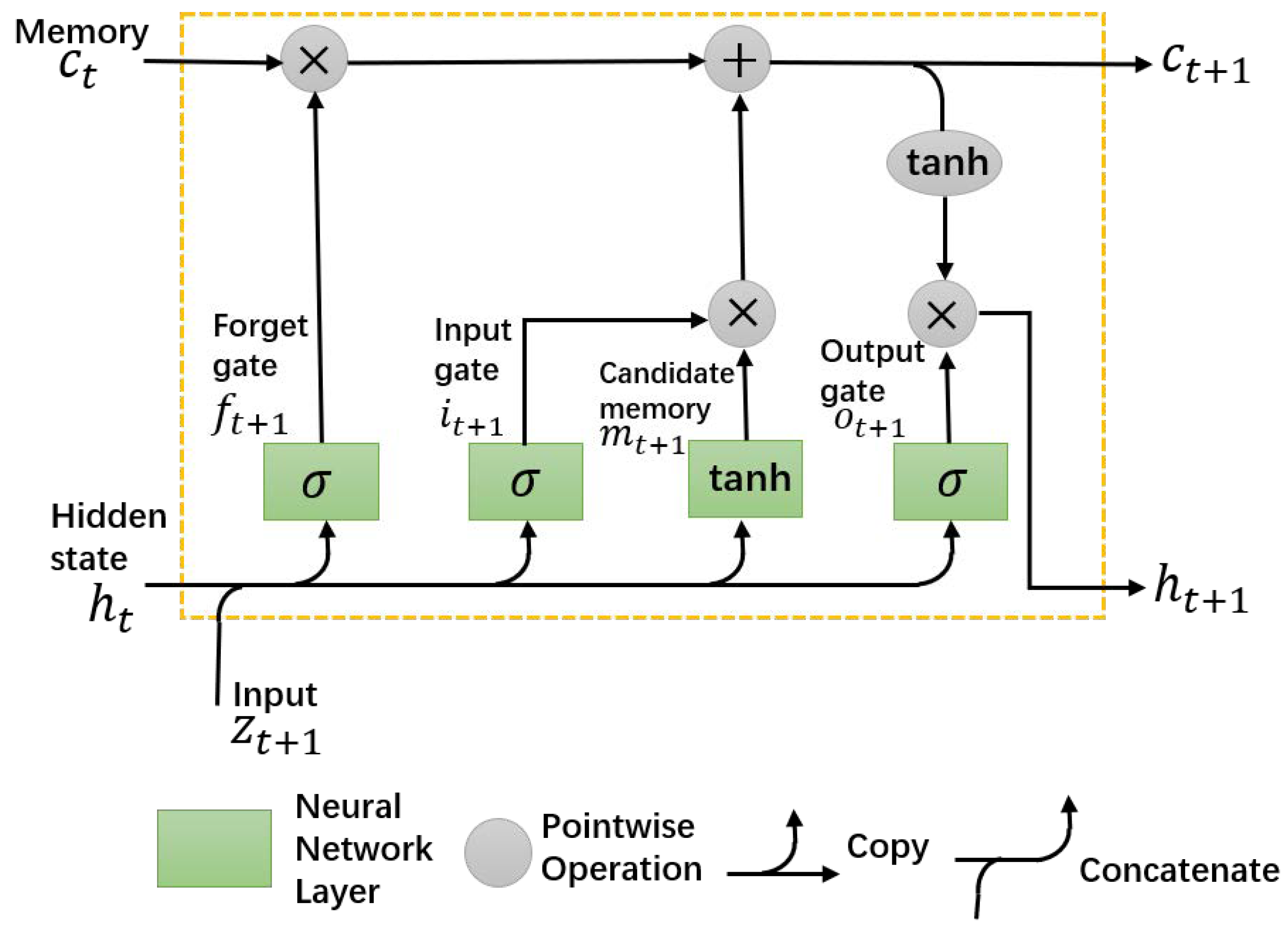
As illustrated in Figure 2, each LSTM unit has three gates, i.e., output gate $o_{t+1}$, input gate $i_{t+1}$, and forget gate $f_{t+1}$, to guide the flows of relevant information. It also includes a memory cell $c_t$ and a hidden state $h_t$ at each time step t. The memory cell is designed to learn how to forget or update the past memories. Therefore, the memory cell and hidden state can be updated as follows:

$$\begin{array}{cc}\hfill f_{t+1}& =\sigma \left(W_f•\left[h_t,z_{t+1}\right]+b_f\right)\hfill \\ \hfill i_{t+1}& =\sigma \left(W_i•\left[h_t,z_{t+1}\right]+b_i\right)\hfill \\ \hfill o_{t+1}& =\sigma \left(W_o•\left[h_t,z_{t+1}\right]+b_o\right)\hfill \\ \hfill m_{t+1}& =tanh\left(W_m•\left[h_t,z_{t+1}\right]+b_m\right)\hfill \\ \hfill c_{t+1}& =f_{t+1}\ast c_t+i_{t+1}\ast m_{t+1}\hfill \\ \hfill h_{t+1}& =o_{t+1}\ast tanh\left(c_{t+1}\right)\hfill \end{array}$$

(2)

where $\left[h_t,z_{t+1}\right]$ represents the concatenation of current hidden state $h_t$ and the input $z_{t+1}$. The weight matrices for the forget, input, output, and memory gates are $W_f$, $W_i$, $W_o$, and $W_m$, respectively. The sigmoid function $\sigma \left(q\right)={\left(1+e^{-q}\right)}^{-1}$ will squash the input q to [0, 1]. In the proposed framework, the final output of the LSTM denotes the probability of each patch being tumorous.

3.3. Optimize with Spatial Constraint

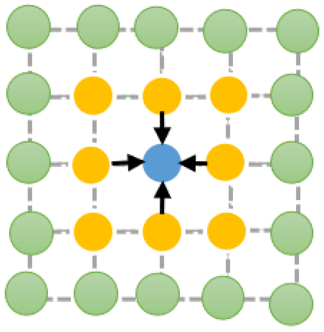
The predicted label, in fact, may not only depend on the current input alone, but also is related to its neighbors in the residing spatial domain, as shown in Figure 3. Given an image patch and its neighbors, in order to predict their categories, this paper proposes a new spatial constraint loss function to further model the spatial structure information in the loss layer.

Let $\phi \left(•\right)$ denote the learned classifier of the proposed method, $y^{*}$ and $y^n$$(n=1,$$2,\cdots ,N)$ represent the ground truth labels of current image patch $x^{*}$ and its neighbors $x^n$$\left(n=1,2,\cdots ,N\right)$, respectively. Ideally, the predictions of patches should be consistent with their ground truth labels. That is, $\left|\phi \left(x^{*}\right)-\phi \left(x^n\right)\right|$ should be smaller when $y^{*}=y^n$. Otherwise, $\left|\phi \left(x^{*}\right)-\phi \left(x^n\right)\right|$ should be larger if $y^{*}\ne y^n$.

In the experiments, tumorous and normal patches are labeled as 1 and 0, respectively.

For patches with the same label, the predicted loss is defined as:

$$L_{same}={\left[\phi \left(x^{*}\right)-\phi \left(x^n\right)\right]}^2$$

(3)

For those patches coming from different categories, the predicted loss is encoded as:

$$L_{dif}=\left[1-\phi \left(x^n\right)\right]\ast \left[1-\phi \left(x^{*}\right)\right]+\phi \left(x^n\right)\ast \phi \left(x^{*}\right)$$

(4)

By integrating Equations (3) and (4), the spatial constraint loss is defined as:

$$L_{spatial}=\frac{1}{N}\sum _{n=1}^N\left[\left(1-\left|y^{*}-y^n\right|\right)\ast L_{same}+\left|y^{*}-y^n\right|\ast L_{dif}\right]$$

(5)

Through minimizing $L_{spatial}$, $L_{same}$ enforces the predictions of $x^{*}$ and $x^n$ to be similar when $y^{*}=y^n$, whereas $L_{dif}$ makes the learned classifier $\phi \left(•\right)$ maximally distinguish $x^{*}$ and $x^n$ if they belong to different categories.

Finally, for the whole training dataset, the optimization objective of the proposed framework is defined as:

$$min\sum _{x^{*}\in D_{train}}\left(L_{CE}+\beta L_{spatial}\right)$$

(6)

where $D_{train}$ denotes the training dataset, $L_{CE}$ is the cross-entropy loss, and hyper-parameter $\beta$ is cross-validated in the experiments.

In order to solve Equation (6), stochastic gradient descent (SGD) is employed with mini-batch to train the deep network. The parameters of the network are updated by back-propagation (BP) strategy.

After generating the probability map of the WSI, the non-maxima suppression algorithm [26,27] is applied to obtain the coordinates of cancer metastases, which repeats two steps until there are no values larger than a certain threshold in the heatmap: (1) search the maximum and its corresponding coordinate; (2) all values in the range of a given radius around the maximum are set to 0.

4. Experiments

4.1. Experimental Setup

Extensive experiments are conducted on the Camelyon16 challenge dataset (https://camelyon17.grand-challenge.org/Data/, accessed on 15 July 2021), which was obtained from two different institutes: University Medical Centre Utrecht (Utrecht UMC) and Radboud University Medical Centre (Radboud UMC). These two medical centers utilize different digital slide scanners to produce the TIF WSIs. The TIF WSIs from Utrecht UMC were created with a 40× objective lens (level-0 pixel size, 0.226 × 0.226 $\mathsf{\mu }$m) through a digital slide scanner (NanoZoomerXR Digital slide scanner C12000-01; Hamamatsu Photonics). The TIF WSIs from Radboud UMC were created with a 20× objective lens (level-0 pixel size, 0.243 × 0.243 $\mathsf{\mu }$m) through a digital slide scanner (Pannoramic 250 Flash II; 3D Histech). The Camelyon16 challenge dataset contains 400 TIF WSIs in total, including 110 tumorous and 160 normal WSIs for training, and 50 tumorous and 80 normal WSIs for test. Among the test WSIs, Test_049 and Test_114 are excluded from the evaluation, as noted by the Camelyon16 organizers. Pathologists have carefully annotated the cancer metastasis locations and regions in the format of binary mask, with a few exceptions reported in [27].

Most WSIs are larger than 60,000 pixels × 100,000 pixels. The size of the whole Camelyon16 dataset is approximately 700 gigabytes. The WSIs are usually saved in a pyramid structure of multi-resolution, with several down-sampled versions of each source image [28]. The source image with the highest resolution is labeled as level-0, whereas other down-sampled images are labeled as level-1 to level-n.

Given a test WSI, the goal is to detect whether this slide includes tumors and locate the areas of these tumors. The model is trained with smaller image patches extracted from the slides, due to the huge size and limited number of slides. A patch is labeled to be tumorous if there is at least one pixel marked as a tumor within the patch area. In general, just a tiny part of the slide includes biological tissue of interest, whereas the majority is background and fat. To reduce computation, the Otsu algorithm [29] is applied to remove the background regions of every training slide.

Training the model was challenging because of the tumorous class imbalance among the large number of patches. There are 10,000 to 400,000 patches (median 90,000) in each slide. However, only 20 to 150,000 tumorous patches (median 2000) are found in each tumor slide. The proportion of tumorous patches is between 0.01% and 70% (median 2%). An effective sampling strategy is adopted to avoid bias towards slides that include more patches (both normal and tumorous). First, “normal” or “tumorous” class is selected with the same probability. Second, a slide containing this class of patches is selected uniformly at random, and then patches are sampled from that slide. In comparison, several existing approaches pre-sampled a number of patches from each slide [30], which restricts the diversity of the training patches.

In the training stage, several strategies of data augmentation are applied to increase the samples of tumorous patch. The input patches are rotated by four multiples of 90°, then flipped left to right, and rotations are repeated. As pathological slides have no canonical directions, the eight directions are all valid. In addition, color jitter is added using torchvision tranforms with the parameters used in [27,31]: hue with a maximum delta of 0.04, saturation with a maximum delta of 0.25, contrast with a maximum delta of 0.75, and brightness with a maximum delta of 64/255. By subtracting 128 and dividing 128, the pixel values of patches are normalized. The proposed approach is implemented using PyTorch-1.6.0 [32] and trained using NVIDIA GeForce GTX 2080 Ti GPU. In order to optimize the whole architecture, RMSProp [33] is employed with the learning rate of 0.01 and momentum of 0.9.

In the test stage, a tumorous probability heatmap is generated by performing prediction over patches in a sliding window, with a stride of 64 across the whole slide. For every patch, rotations and left–right flip are applied to generate the prediction results in the eight directions, and the patch-level tumor prediction is finally obtained by averaging the prediction results in the eight directions. The maximum value in the tumorous probability heatmap is taken as prediction result of each slide.

4.2. Evaluation Metrics

Two Camelyon16 evaluation metrics are employed to assess the performance of tumor region localization and WSI classification. The area under receiver operating characteristic (area under ROC, AUC) [34] is utilized for the evaluation of slide-level classification performance. The free response operating characteristic (FROC) curve [35] is utilized for performance evaluation in tumor detection and localization.

The FROC curve is defined as a sensitivity plot versus the average number of false positives per image under various probability truncation values. To be specific, for each heatmap, a list of coordinates and related predictions will first be generated. The maximum prediction value is recorded among all the coordinates within each annotated tumor area. FPs are the number of coordinates that fall outside tumor areas. The FROC score is defined as the average sensitivity at six predefined false positive rates: 1/4, 1/2, 1, 2, 4, and 8 false positives. Higher average FROC score means better detection performance.

In order to produce the points for FROC calculation, Camelyon16 challenge winner thresholded the heatmap to generate a bitmask, and recorded a single prediction value for every connected component in the bitmask. Instead, based on a certain probability map, the non-maxima suppression algorithm [26,27] is employed to get cancer metastasis coordinates.

4.3. Results and Discussion

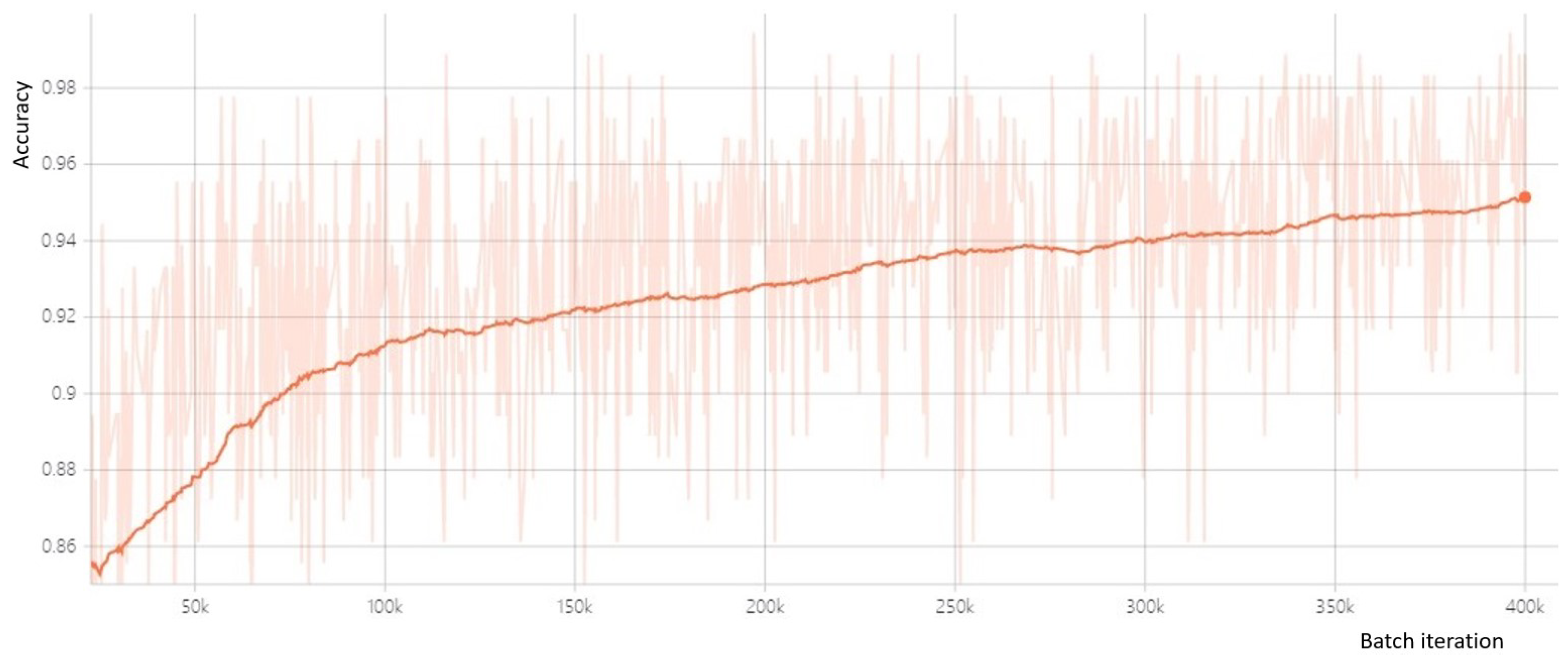
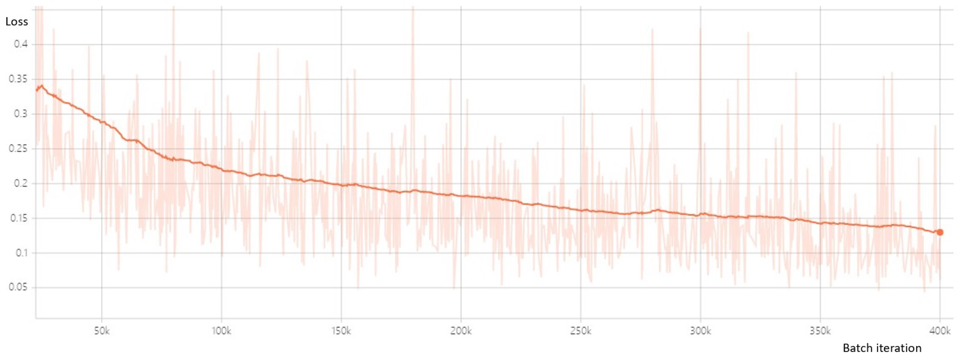
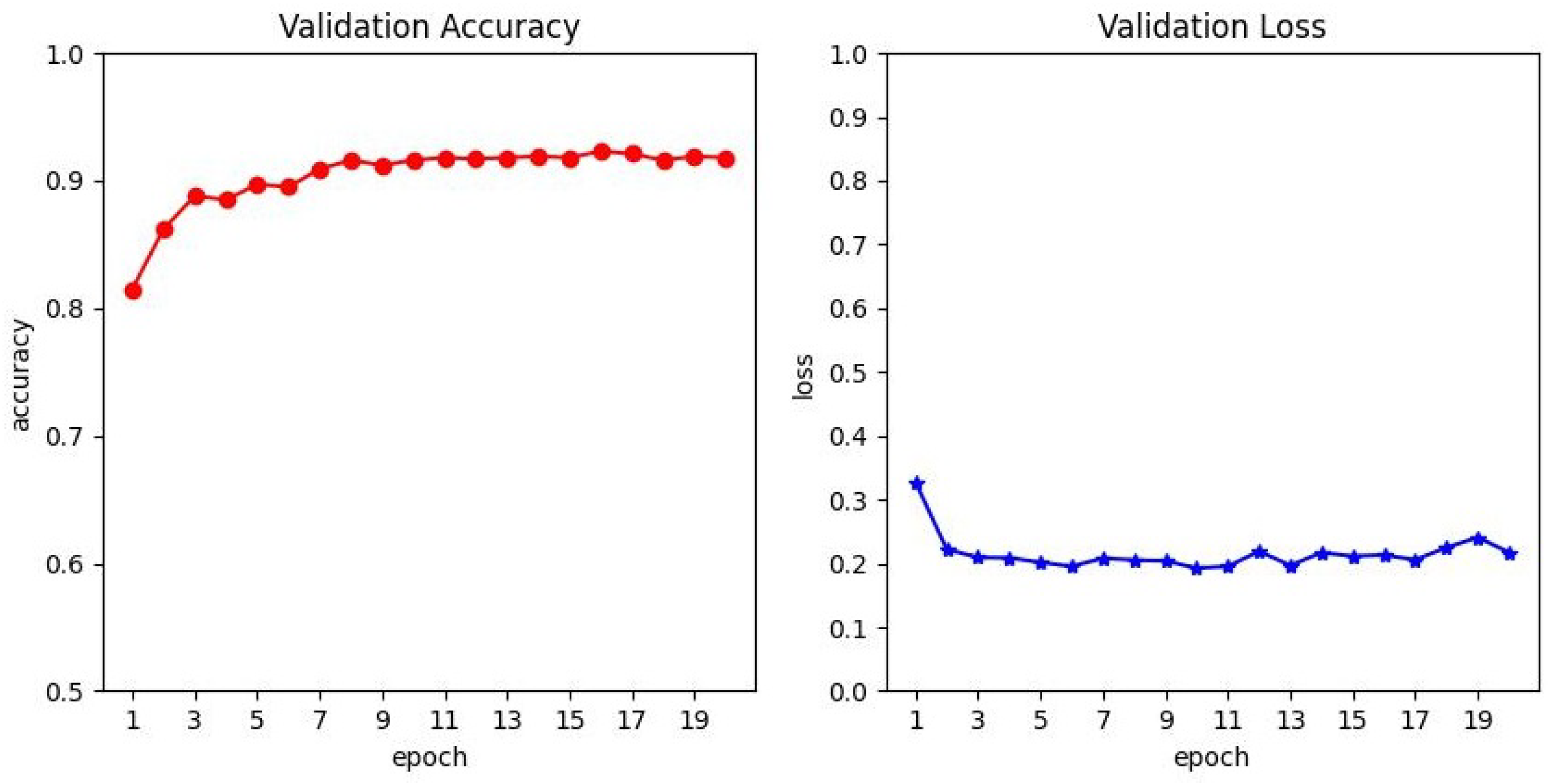
First, the convergence speed of the proposed method is validated through the loss and accuracy on the training and validation sets, as shown in Figure 4, Figure 5 and Figure 6.

The effectiveness of the proposed spatially structured constraint is also evaluated. Compared with the baseline ResNet-34, the proposed model is composed of ResNet-34 and LSTM. The proposed method employed both LSTM and spatial constraint loss to learn the 2D spatial relationships between adjacent patches. It is observed from

Table 1. Performance evaluation of the spatially structured constraint.

Methods	FROC Score	AUC Score
Baseline ResNet-34	0.7463	0.9524
The proposed framework without spatial constraint loss	0.7542	0.9681
The proposed framework	0.8093	0.9834

that after adding the spatial constraint in the network, the FROC score is improved by 6.3%, compared with the baseline ResNet-34. It is implied the network architecture without spatially structured information only obtains a suboptimal solution. In addition, the spatially structured constraint, as an effective “plug-in”, can also be seamlessly integrated into various network architectures. For the case without spatial constraint loss, it only utilized the cross-entropy loss during the training. The grid of patch representations is transformed into a sequence as the input of LSTM, so only 1D spatial relationships between neighboring patches are considered. That is why it only marginally improves the performance (approximately 1%), compared with the baseline ResNet-34.

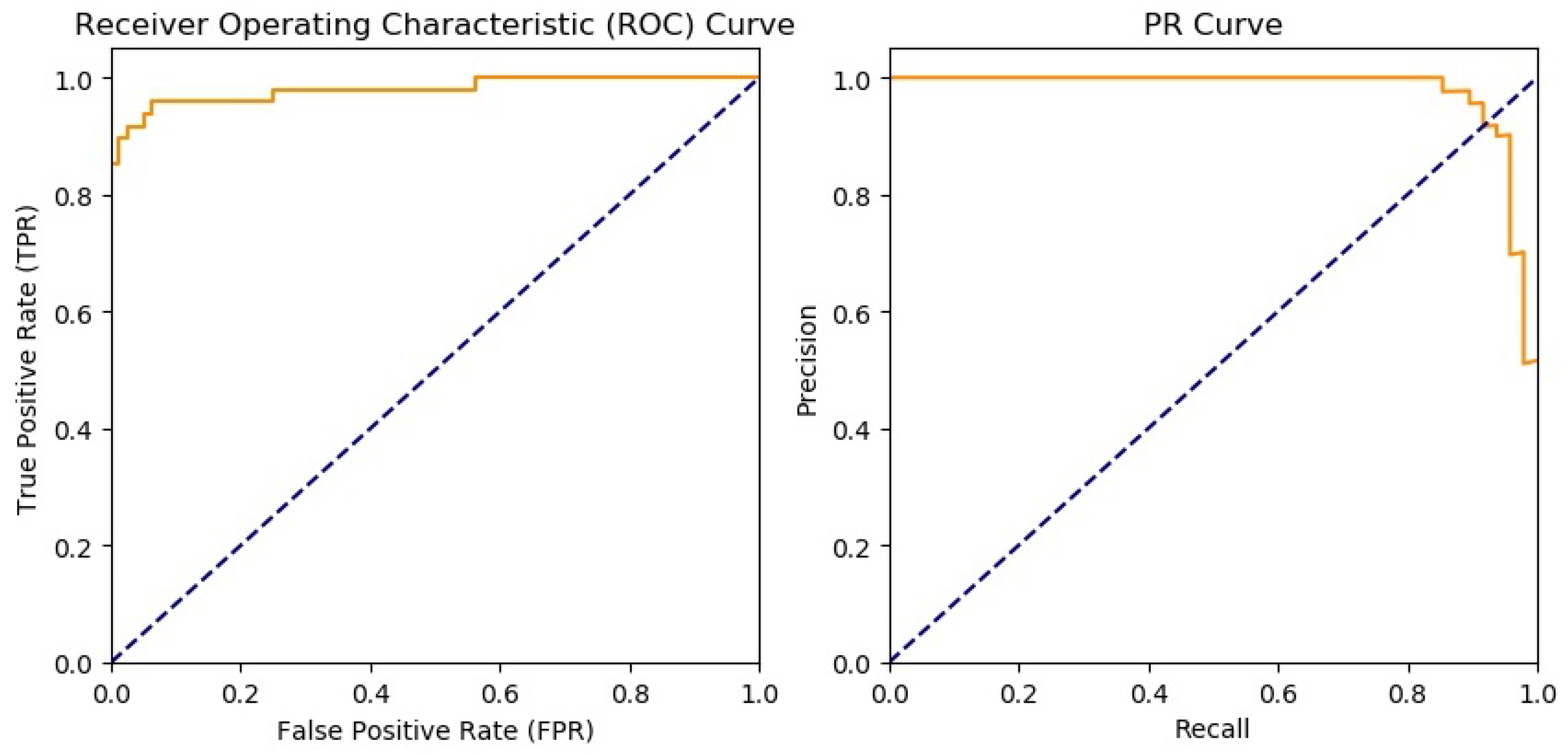
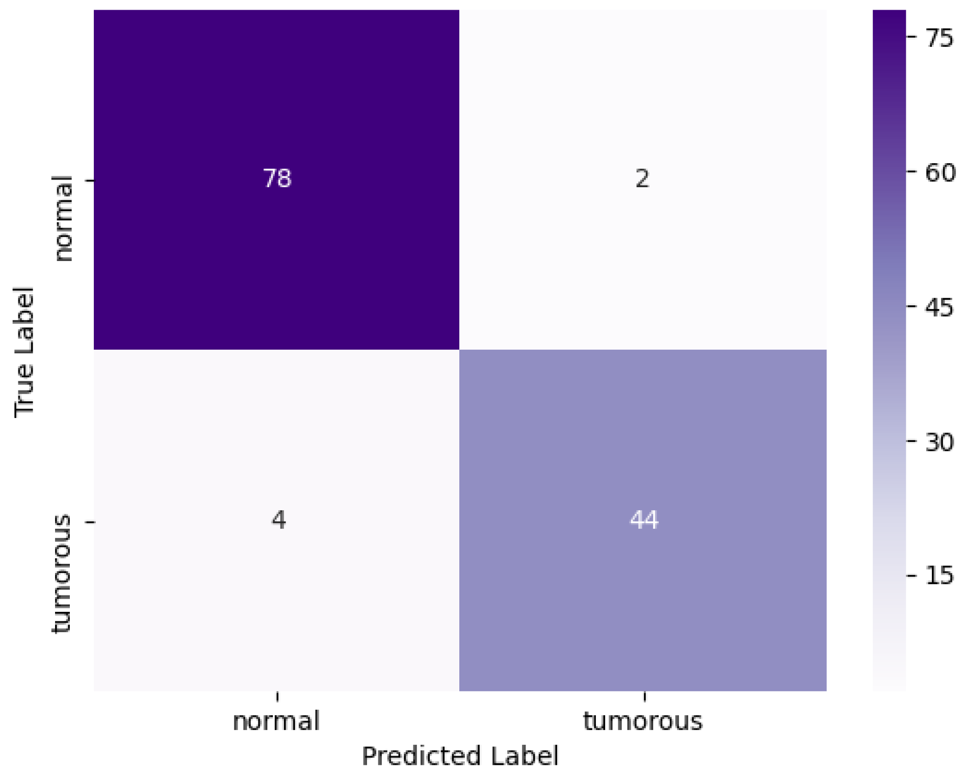
Furthermore, the approach is compared with several state-of-the-art approaches, which were submitted by different top institutions and organizations to the Camelyon16 challenge. It is observed from

Table 2. Performance evaluation on Camelyon16 dataset.

Approaches	FROC Score	AUC Score
Human performance	0.7325	0.9660
C Radboud Uni. (DIAG)	0.5748	0.7786
Middle East Tech. Uni.	0.3889	0.8642
L HMS, Gordan Center, MGH	0.7600	0.9763
NLP LOGIX co. USA	0.3859	0.8298
EXB Research co.	0.5111	0.9156
DeepCare Inc.	0.2439	0.8833
University of Toronto	0.3822	0.8149
The proposed framework	0.8093	0.9834

that the proposed approach is superior to other methods in both tumor localization and WSI classification tasks. In comparison with other state-of-the-art methods, which employed different CNN models to extract patch feature and did not take into account spatial correlations among image patches, the proposed approach not only extracts discriminative feature for each image path, but also embeds spatial information between adjacent neighbors into the image patch to make better predictions. It should be noted that detection performance of the proposed approach outperformed that from pathologists by about 7%, which highlights the proposed approach’s capability to detect metastasis in lymph node biopsies. The PR and ROC curves of the proposed method are shown in Figure 7, where precision is 0.9565, recall = 0.9167, F1 score = 0.9362, balanced accuracy = 0.9458, accuracy = 0.9531. The confusion matrix of the proposed method, shown in Figure 8, provides better insight into the achieved results. It is demonstrated that the proposed approach not only provides an objective solution, but also achieves more accurate results in localization.

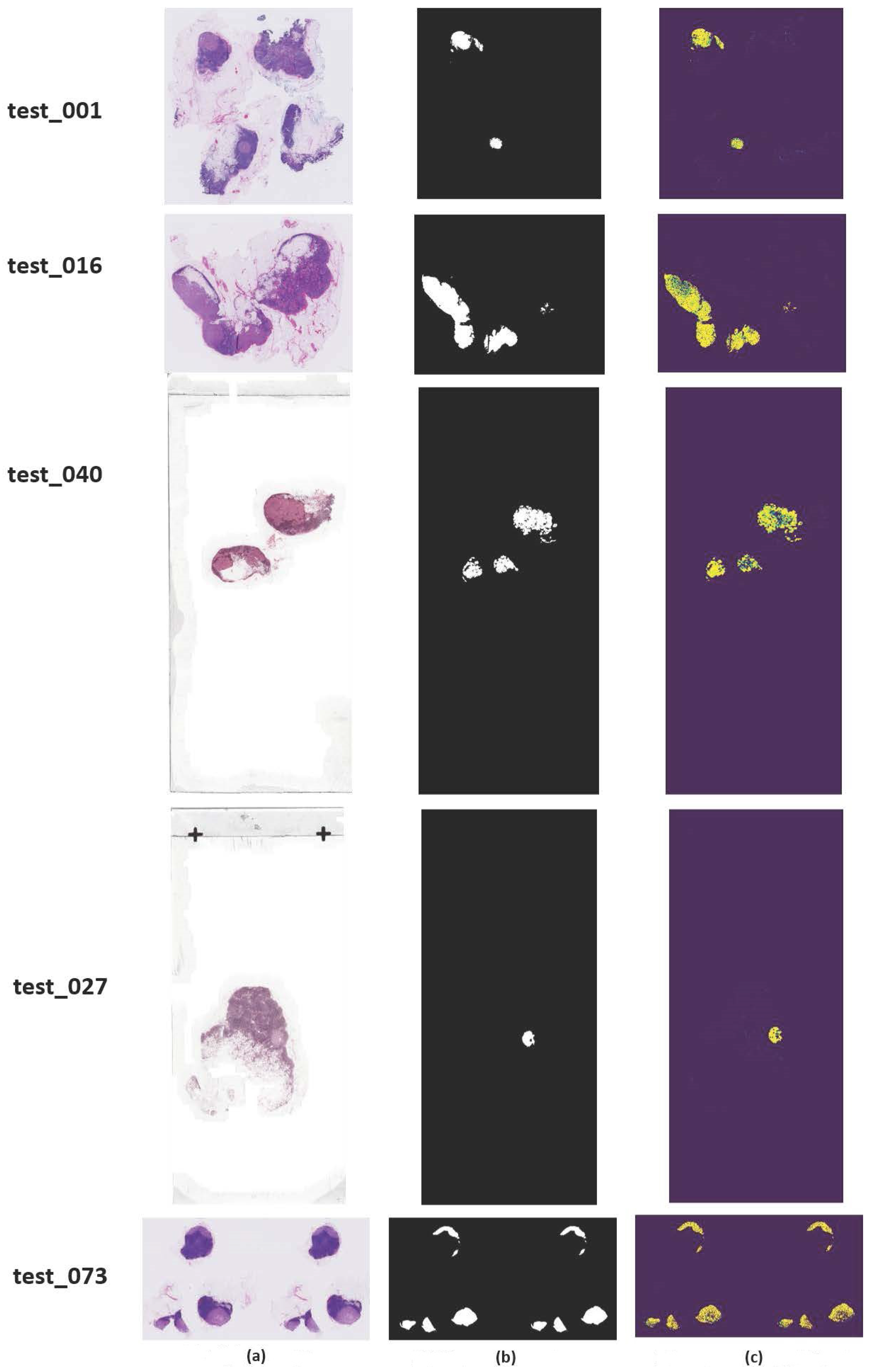
Several detection probability results from the proposed framework are also displayed to emphasize the excellent performance of this method. It can be observed from Figure 9 that the proposed approach generates detection probability maps with better visual quality, and metastasis detection results of the proposed approach in the third column have excellent agreement with the ground truth annotations in the second column generated by the experienced pathologists. It is obvious that the proposed approach can detect metastases very well within the whole-slide images.

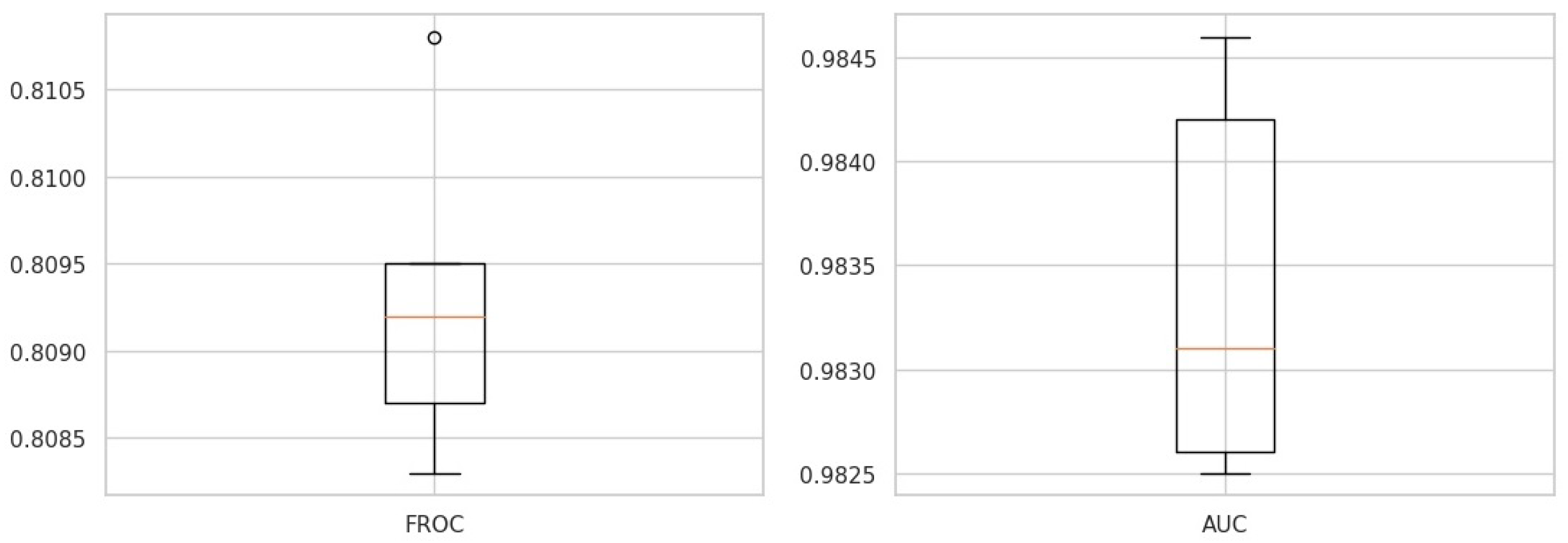
The diversity of FROC score and AUC score for the proposed method is shown in the box and whiskers diagrams. It can be seen from Figure 10 that the proposed method exhibits stable behavior with a relatively low standard deviation value.

5. Conclusions

This paper proposes an effective spatially sensitive learning network for cancer metastasis identification in whole-slide images. In addition, a novel spatial loss function is designed to integrate the spatial constraint into the network for more accurate detection. Specifically, the proposed method incorporates a CNN feature extractor, LSTM, and spatial constraint loss into a unified framework. Consequently, the proposed method not only takes into account the spatial dependencies among adjacent patches through LSTM and spatial loss function, but the CNN feature extractor also benefits from the joint learning framework. Extensive experiments on the benchmark Camelyon2016 Grand Challenge dataset demonstrate that the proposed approach obtains better performance than state-of-the-art methods in cancer metastasis identification.

The proposed approach utilizes the patch-based classification and analyzes gigapixel whole-slide images in a sliding window with a scanning stride of 64 at the resolution of level-6. When scanning the whole-slide image at a higher resolution (i.e., level-0) for micro-metastases, it will take much more time and computation resources, which is not suitable for clinical practice. Therefore, how to dramatically improve the inference efficiency while maintaining competitive accuracy is an important research direction for whole-slide image analysis in future. Furthermore, it is expected that the proposed model can be applied in other kinds of medical image analysis, as spatial structures generally exist in various medical images (e.g., cardiac MRI).

References

1. Bray, F.; Ferlay, J.; Soerjomataram, I.; Siegel, R.L.; Torre, L.A.; Jemal, A. Global cancer statistics 2018: GLOBOCAN estimates of incidence and mortality worldwide for 36 cancers in 185 countries. CA Cancer J. Clin. 2018, 68, 394–424. [Google Scholar] [CrossRef] [Green Version]
2. Apple, S.K. Sentinel lymph node in breast cancer: Review article from a pathologist’s point of view. J. Pathol. Transl. Med. 2016, 50, 83–95. [Google Scholar] [CrossRef] [Green Version]
3. Ramos-Vara, J.A. Principles and methods of immunohistochemistry. Methods Mol. Biol. 2011, 691, 83–96. [Google Scholar]
4. Humphreys, G.; Ghent, A. World laments loss of pathology service. Bull. World Health Organ. 2010, 88, 564–565. [Google Scholar]
5. Litjens, G.; Sánchez, C.; Timofeeva, N.; Hermsen, M.; Nagtegaal, I.; Kovacs, I.; Kaa, H.; Bult, P.; Ginnneken, B.V.; Laak, J. Deep learning as a tool for increased accuracy and efficiency of histopathological diagnosis. Sci. Rep. 2016, 6, 26286. [Google Scholar] [CrossRef] [Green Version]
6. Spanhol, F.A.; Oliveira, L.S.; Petitjean, C.; Heutte, L. A dataset for breast cancer histopathological image classification. IEEE Trans. Biomed. Eng. 2015, 63, 1455–1462. [Google Scholar] [CrossRef] [PubMed]
7. Cruz-Roa, A.A.; Ovalle, J.; Madabhushi, A.; Osorio, F. A Deep Learning Architecture for Image Representation, Visual Interpretability and Automated Basal-Cell Carcinoma Cancer Detection. In Proceedings of the 16th International Conference on Medical Image Computing and Computer Assisted Intervention, Nagoya, Japan, 22–26 September 2013; pp. 403–410. [Google Scholar]
8. Kandemir, M.; Hamprecht, F. Computer-aided diagnosis from weak supervision: A benchmarking study. Comput. Med. Imaging Graph. 2015, 42, 44–50. [Google Scholar] [CrossRef] [PubMed]
9. Alom, M.Z.; Taha, T.M.; Yakopcic, C.; Westberg, S.; Asari, V.K. The history began from alexnet: A comprehensive survey on deep learning approaches. arXiv 2018, arXiv:1803.01164. [Google Scholar]
10. Litjens, G.; Kooi, T.; Bejnordi, B.E.; Setio, A.A.; Ciompi, F.; Ghafoorian, M.; Laak, J.A.; Ginneken, B.; Sánchez, C.I. A survey on deep learning in medical image analysis. Med. Image Anal. 2017, 42, 60–88. [Google Scholar] [CrossRef] [PubMed] [Green Version]
11. Basha, J.; Bacanin, N.; Vukobrat, N.; Zivkovic, M.; Venkatachalam, K.; Hubálovský, S.; Trojovský, P. Chaotic Harris Hawks Optimization with Quasi-Reflection-Based Learning: An Application to Enhance CNN Design. Sensors 2021, 21, 6654. [Google Scholar] [CrossRef]
12. Manzo, M.; Pellino, S. Bucket of Deep Transfer Learning Features and Classification Models for Melanoma Detection. J. Imaging 2020, 6, 129. [Google Scholar] [CrossRef]
13. Spanhol, F.; Oliveira, L.S.; Cavalin, P.R.; Petitjean, C.; Heutte, L. Deep features for breast cancer histopathological image classification. In Proceedings of the IEEE International Conference on Systems, Man, and Cybernetics, Banff, AB, Canada, 5–8 October 2017; pp. 1868–1873. [Google Scholar]
14. Bayramoglu, N.; Kannala, J.; Heikkilä, J. Deep learning for magnification independent breast cancer histopathology image classification. In Proceedings of the 23rd International Conference on Pattern Recognition (ICPR), Cancun, Mexico, 4–8 December 2016; pp. 2440–2445. [Google Scholar]
15. Guo, Y.; Dong, H.; Song, F.; Zhu, C.; Liu, J. Breast Cancer Histology Image Classification Based on Deep Neural Networks. In International Conference Image Analysis and Recognition; Springer: Cham, Switzerland, 2018; Volume 10882, pp. 827–836. [Google Scholar]
16. Ehteshami Bejnordi, B.; Linz, J.; Glass, B.; Mullooly, M.; Gierach, G.; Sherman, M.; Karssemeijer, N.; van der Laak, J.; Beck, A. Deep learning-based assessment of tumor-associated stroma for diagnosing breast cancer in histopathology images. In Proceedings of the IEEE 14th International Symposium on Biomedical Imaging, Melbourne, VIC, Australia, 18–21 April 2017; pp. 929–932. [Google Scholar]
17. Lin, H.; Chen, H.; Dou, Q.; Wang, L.; Qin, J.; Heng, P.A. ScanNet: A Fast and Dense Scanning Framework for Metastatic Breast Cancer Detection from Whole-Slide Images. In Proceedings of the IEEE Winter Conference on Applications of Computer Vision (WACV), Lake Tahoe, NV, USA, 12–15 March 2018; pp. 539–546. [Google Scholar]
18. Lin, H.; Chen, H.; Graham, S.; Dou, Q.; Rajpoot, N.; Heng, P.A. Fast scannet: Fast and dense analysis of multi-gigapixel whole-slide images for cancer metastasis detection. IEEE Trans. Med. Imaging 2019, 38, 1948–1958. [Google Scholar] [CrossRef] [Green Version]
19. Xie, J.; Liu, R.; Luttrell, J.; Zhang, C. Deep Learning Based Analysis of Histopathological Images of Breast Cancer. Front. Genet. 2019, 10, 80. [Google Scholar]
20. de Matos, J.; de Souza Britto, A.; Oliveira, L.; Koerich, A.L. Double Transfer Learning for Breast Cancer Histopathologic Image Classification. In Proceedings of the International Joint Conference on Neural Networks (IJCNN), Budapest, Hungary, 14–19 July 2019; pp. 1–8. [Google Scholar]
21. Kassani, S.H.; Kassani, P.H.; Wesolowski, M.J.; Schneider, K.A.; Deters, R. Breast Cancer Diagnosis with Transfer Learning and Global Pooling. In Proceedings of the International Conference on Information and Communication Technology Convergence (ICTC), Jeju, Korea, 16–18 October 2019; pp. 519–524. [Google Scholar]
22. Zanjani, F.G.; Zinger, S.; With, P. Cancer detection in histopathology whole-slide images using conditional random fields on deep embedded spaces. In Proceedings of the Digital Pathology, Houston, TX, USA, 6 March 2018. [Google Scholar]
23. Kong, B.; Xin, W.; Li, Z.; Qi, S.; Zhang, S. Cancer Metastasis Detection via Spatially Structured Deep Network. In International Conference Image Analysis and Recognition; Springer: Cham, Switzerland, 2017; pp. 236–248. [Google Scholar]
24. He, K.; Zhang, X.; Ren, S.; Sun, J. Deep Residual Learning for Image Recognition. In Proceedings of the IEEE Conference on Computer Vision and Pattern Recognition, Las Vegas, NA, USA, 27–30 June 2016. [Google Scholar]
25. Sepp Hochreiter, J.S. Long short-term memory. Neural Comput. 1997, 9, 1735–1780. [Google Scholar] [CrossRef]
26. Ciresan, D.C.; Giusti, A.; Gambardella, L.M.; Schmidhuber, J. Mitosis detection in breast cancer histology images with deep neural networks. In Medical Image Computing and Computer-Assisted Intervention; Springer: Berlin/Heidelberg, Germany, 2013; Volume 16, pp. 411–418. [Google Scholar]
27. Liu, Y.; Gadepalli, K.; Norouzi, M.; Dahl, G.E.; Kohlberger, T.; Boyko, A.; Venugopalan, S.; Timofeev, A.; Nelson, P.Q.; Corrado, G.S. Detecting cancer metastases on gigapixel pathology images. arXiv 2017, arXiv:1703.02442. [Google Scholar]
28. Goode, A.; Gilbert, B.; Harkes, J.; Jukie, D.; Satyanarayanan, M. Openslide: A vendor-neutral software foundation for digital pathology. J. Pathol. Inform. 2013, 4, 27. [Google Scholar] [CrossRef]
29. Otsu, N. A threshold selection method from gray-level histograms. IEEE Trans. Syst. Man Cybern. 1979, 9, 62–66. [Google Scholar]
30. Wang, D.; Khosla, A.; Gargeya, R.; Irshad, H.; Beck, A.H. Deep learning for identifying metastatic breast cancer. arXiv 2016, arXiv:1606.05718. [Google Scholar]
31. Yi, L.; Wei, P. Cancer Metastasis Detection With Neural Conditional Random Field. arXiv 2018, arXiv:1806.07064. [Google Scholar]
32. Paszke, A.; Gross, S.; Chintala, S.; Chanan, G.; Yang, E.; Devito, Z.; Lin, Z.; Desmaison, A.; Antiga, L.; Lerer, A. Automatic Differentiation in PyTorch. In Proceedings of the 31st Conference on Neural Information Processing Systems (NIPS 2017) Autodiff Workshop, Long Beach, CA, USA, 9 December 2017. [Google Scholar]
33. Tijmen, T.; Hinton, G. Lecture 6.5-rmsprop: Divide the gradient by a running average of its recent magnitude. COURSERA Neural Netw. Mach. Learn. 2012, 4, 26–31. [Google Scholar]
34. Hanley, J.A.; Mcneil, B.J. The meaning and use of the area under a receiver operating characteristic (roc) curve. Radiology 1982, 143, 29–36. [Google Scholar] [CrossRef] [Green Version]
35. Chakraborty, D.P. Maximum likelihood analysis of free-response receiver operating characteristic (froc) data. Med. Phys. 1989, 16, 561–568. [Google Scholar] [CrossRef] [PubMed]
Figure 1. Overview of the proposed framework. CNN and LSTM are two important components of this framework. When a grid of patches is input, the CNN feature extractor will encode every patch as a given-length vector representation. Given the grid of patch representations, the LSTM component models the spatial relationships between adjacent patches and outputs the probability of every patch being tumorous. In addition, spatial constraint is also imposed on the loss function to further improve the performance.
Mathematics 10 02657 g001
Figure 2. Structure of a single LSTM cell.
Mathematics 10 02657 g002
Figure 3. An illustration of a spatially structured constraint. The blue circle represents the center of an image patch; the centers of its neighboring patches are represented by yellow circles.
Mathematics 10 02657 g003
Figure 4. Patch classification accuracy of each batch throughout training.
Mathematics 10 02657 g004
Figure 5. Patch training loss of each batch.
Mathematics 10 02657 g005
Figure 6. Patch loss and accuracy on validation set.
Mathematics 10 02657 g006
Figure 7. PR curve and ROC curve of the proposed method.
Mathematics 10 02657 g007
Figure 8. Confusion matrix of the proposed method.
Mathematics 10 02657 g008
Figure 9. Metastasis identification examples using the proposed approach. (a) original image; (b) ground truth annotation; (c) predicted probability map.
Mathematics 10 02657 g009
Figure 10. Diversity analysis for the proposed method.
Mathematics 10 02657 g010