On the Constrained Solution of RBF Surface Approximation

Abstract

In this contribution, a scattered data approximation problem, chosen from the literature and using the Radial Basis Function (RBF) approach, is considered for the application of point cloud modelling. Three solutions are investigated for the approximation problem. First, a technique known from the literature is investigated using a linear combination of thin-plate splines and linear polynomials, with additional constraint equations. Then, using the same approximation function as before, a technique is developed for a rigorous consideration of the constraint equations. Finally, a technique is presented in which the approximation function consists only of a linear combination of thin-plate splines, without the introduction of linear polynomials and constraint equations. In addition, some interpolation problems with the RBF approach are discussed to present the differences between an interpolation with thin-plate splines only and an interpolation with thin-plate splines together with linear polynomials and constraint equations. Numerical examples are given to illustrate and discuss the solutions from the different techniques.

1. Introduction

Nowadays, the use of 3D laser scanning technology is widespread in various applications for digitizing real world objects. The acquired point cloud consists of measured coordinates in ${\mathrm{I}\mathrm{R}}^3$ of numerous points. The number of points can be up to several millions, resulting in a huge data set. Moreover, the points are considered unorganized and scattered, which means that there is no specific structure or topological relation between them. Hence, the points and their coordinates are not sufficient to provide additional information about the object. As Bureick et al. [1] mentioned, only by modelling the geometric information can further analysis be performed, and several questions which could not be addressed before can be answered. For instance, in Computer-Aided Design (CAD) or in deformation analysis, a surface approximation with a continuous mathematical function is required, as, e.g., pointed out by Bureick et al. [1]. Therefore, modelling the point cloud is a necessity and surface approximation is taken into account.

There are numerous approaches to approximate a surface involving functions such as polynomials, splines, B–splines, etc. For instance, Bureick et al. [1] presented surface approximations based on polynomials, Bézier, B-splines and Non-Uniform Rational B-splines (NURBS). Each of these approaches has its advantages and some disadvantages. In this article, the Radial Basis Function (RBF) approach is discussed. This choice is motivated by typical tasks in Geodesy and Geoinformation Science. There, the challenge is often to model point clouds that include a very large number of points in the 3D space dimension with unorganized points (scattered points), which point clouds have been captured with laser scanners or photogrammetric methods. As Buhmann [2] (p. 1ff.) explained, when the functions to be approximated (a) depend on many variables or parameters, (b) are defined by possibly very many data, and (c) the data are scattered in their domain, then the Radial Basis Function approach is especially well-suited.

Another advantage of the Radial Basis Function approach is that it is a meshfree approach. In contrast to some other approaches that require a mesh such as those using wavelets, multivariate splines, finite elements, etc., as Wendland [3] (p. ix) explained. According to Fasshauer [4] (p. 1), mesh generation can be the most time-consuming part of any mesh-based numerical approach. Moreover, he continued, a meshfree approach is often better suited to cope with changes in the geometry of the domain of interest (e.g., free surfaces and large deformations) than approaches such as finite elements.

Mainly, in this article, the approximation of point clouds is considered, since with high point density and the fact that measured coordinates are subject to random measurement errors, interpolation is no longer appropriate. In the case of interpolation, measurement errors and other abrupt changes in the data points would be modelled, resulting in a strongly oscillating modelled surface. Nevertheless, some numerical examples of interpolation, with a few data points, will be presented to reveal the effect of the applied technique.

For the scattered data approximation problem with the RBF approach, an approximation function is built that consists of a linear combination of radial basis functions. Each radial “basis” function $\mathsf{\Phi }\left(\right||·|{|}_2)$ is centered at each fixed center point, and by composition with the Euclidean norm $\left|\right|·{\left|\right|}_2$, $\mathsf{\Phi }$ is radially (or spherically) symmetric about this center point. A formal definition of a radial function is given by Fasshauer [4] (p. 17). Furthermore, each radial “basis” function is a multivariate function which is based on a univariate continuous “basic” function $\varphi \left(r\right)$. The basic function is used to derive all the radial basis functions in the approximation function. The terminology “basis” and “basic” function is adopted from the textbook by Fasshauer [4] (p. 18). Based on the contribution by Flyer et al. [5],

Table 1. Basic functions.

Name	$\mathit{\varphi }\left(\mathit{r}\right)$
Gaussian	${\mathrm{e}}^{-{\left(ϵr\right)}^2}$
Multiquadric	$\sqrt{1+{\left(ϵr\right)}^2}$
Inverse multiquadric	$\frac{1}{\sqrt{1+{\left(ϵr\right)}^2}}$
Thin-plate spline	$r^{2}log\left(r\right)$

shows some of the well-known basic functions, where $ϵ$ is a shape parameter defined by the user.

In this article, the basic function used, namely thin-plate spline, is chosen for the important advantage that no shape parameter is required. Based on the analysis of Fasshauer [4] (p. 23ff.), the value of the shape parameter has a great influence on the numerical stability of the interpolation problem, and if not chosen appropriately, can result in severe ill-conditioning of the interpolation matrix. A sophisticated method is, e.g., presented in the paper by Zheng et al. [6], who used a test differential equation for the selection of a good shape parameter. In the following, a shape parameter-free basic function is preferred. In addition to the previous advantage, the thin-plate spline function, according to Fasshauer [4] (p. 170), has the tendency to produce “visually pleasing” smooth and tight surfaces.

The first appearance of the thin-plate spline function in an interpolation problem was presented by Harder and Desmarais [7] under the name “surface spline” for applications related to aircraft design. Duchon [8] studied their method and extended the mathematical representation based on Hilbert kernel theory, which had a major impact on subsequent research on the interpolation of spline functions with radial basis functions. In his article, Duchon [8] was interested in an interpolating surface with minimal bending energy, which geometrically means that he was aiming for an interpolation that was as flat as possible, that is, as close to a plane as possible. He composed, for this purpose, the interpolating function as a linear combination of thin-plate spline functions with an addition of linear polynomials. Furthermore, condition equations were taken into account to ensure a unique solution.

As Harder and Desmarais [7] explained, the thin-plate spline function has a physical interpretation which is a plate of infinite extend that deforms in bending only. Since the bending energy is represented by the integral of the partial derivatives, the minimal bending energy of the surface that Duchon [8] was interested in is approximately equivalent to the minimal integral curvature, and hence with the minimum of the functional of second derivatives. For this minimisation, Duchon [8] defined a semi-norm in the infinitely dimensional vector subspace of functions of finite energy. Furthermore, since linear polynomials defining a plane are equal to zero in their second derivatives, they are also included in the interpolation function. Finally, Duchon [8] proved that the functions, thin-plate splines and polynomials can be used as a basis for surface interpolation, and the space of this basis is a subspace of the infinite dimensional Hilbert vector space of all real functions of two real variables. Later on, this form of interpolation presented by Duchon [8] was widely used in the literature, for instance, by Buhmann [9], by Wendland [3] (p. 116ff.), by Fasshauer [4] (p. 70ff.), and by Flyer et al. [5], to name a few, when interpolating with thin-plate spline functions.

Here, it should be clarified that this form of interpolation that is adding a series of polynomials to the interpolation function and also considering condition equations is an interpolation technique that was first introduced by Hardy [10], but with different basis functions, under the title “osculating mode”. Specifically, in his article, the interpolation function is constructed as a linear combination of multiquadric functions plus a series of polynomials. Additionally, condition equations were used. Hardy [10] applied this technique for the problem of representing a topographic surface by a continuous function while a set of few discrete data on the surface was given. In his application, he was seeking to minimize horizontal and vertical displacements of the maximum (hilltops) and minimum (depressions) points in the resulting surface of topography. Therefore, he chose an osculating, as he named it, interpolation technique, where the surface coordinates collocate with the data point coordinates, but also surface tangents coincide at specified points. The latter was achieved by the usage of low degree polynomials in the interpolation function. Later on, this interpolation technique was used in various applications, as were described collectively by Hardy [11]. In this article, Hardy [11] named this interpolation technique the multiquadric method.

An additional clarification follows here. In the literature on RBF, the term “condition” equations is usually used, while in the geodetic literature these equations are referred to as “constraint” equations since only unknown parameters (and possibly error-free values) are considered and related to each other. Mikhail [12] (p. 213ff.) explained that constraints for the parameters occur when some or all of the parameters must conform to some relationships arising from either geometric or physical characteristics of the problem. Therefore, in the remainder of this article, these equations will only be referred to as constraint equations.

In this article, it is shown that the approximation problem with the RBF approach, consisting of a linear combination of thin-plate splines, has a unique solution without modifying the approximation function, i.e., without additional polynomials and without constraint equations. The unknown parameters are estimated with the use of the least squares method. Additionally, it is shown that when constraint equations must be introduced, a least squares solution with constraint equations for the unknown parameters can be computed. Moreover, some interpolation problems of a few points, with thin-plate splines, without additional polynomial terms and constraint equations, revealed that they are well-posed. This article is organized as follows.

In Section 2, the theoretical foundations for the solution of the approximation problem with thin-plate splines are shown. The result is a linear least squares adjustment problem, which is well-known, e.g., in Geodesy.

In Section 3, a numerical example from the textbook by Fasshauer [4] is presented. The solution technique used by Fasshauer [4] (p. 170) is described and discussed.

In Section 4, the numerical example of Section 3 is used again. However, the solution is now performed using the adjustment technique presented in Section 2, which allows for the rigorous consideration of the constraint equations.

In Section 5, the numerical example of Section 3 is solved again, but without the addition of the polynomial terms and the constraint equations for the unknown parameters. The solution is obtained based on the theory presented in Section 2.

Section 6 discusses the investigation results of the surface approximations from Section 3, Section 4 and Section 5.

Section 7 contains a comparison of eight interpolation problems with thin-plate splines of four data sets. Finally, in Section 8, conclusions are drawn and some considerations for further investigations are made.

2. The Scattered Data Approximation Problem

In the following, an overdetermined configuration for the surface approximation problem with scattered data using RBF is considered. In this case, the parameters can be determined via least squares adjustment ($L_2$–norm minimisation). First, the ordinary adjustment technique is shown, then the constrained adjustment technique is presented where the solution is obtained with additional consideration of constraint equations for the unknowns. Detailed derivations for the solution of adjustment problems with or without constraint equations can be found in many places in the geodetic literature, e.g., in the textbooks by Dermanis [13] (pp. 4ff., 43ff.), Ghilani and Wolf [14] (pp. 173ff., 388ff.), Mikhail [12] (pp. 159ff., 213ff.) and Niemeier [15] (pp. 112ff., 188ff.), to name a few.

2.1. Ordinary Least Squares Solution

The problem of approximating scattered data is considered, in which a part of the data is regarded as measurements (observations) subject to random errors. If $n>m$, which is that the number of measurements n is larger than the number of unknowns m, the following adjustment problem can be formulated.

A set $\mathcal{X}=\{{\mathbf{x}}_1,\dots ,{\mathbf{x}}_n\}$, with ${\mathbf{x}}_i=(x_i,y_i)\in {\mathrm{I}\mathrm{R}}^2$, named “data sites”, is given. In addition, the corresponding measurements are given as scalar-valued data, denoted by $l_i\in \mathrm{I}\mathrm{R}$ with $i=1,\dots ,n$. Additionally, a set ${\mathcal{X}}_k=\{{\mathbf{x}}_{k_1},...,{\mathbf{x}}_{k_m}\}$, with ${\mathbf{x}}_{k_j}=(x_{k_j},y_{k_j})\in {\mathrm{I}\mathrm{R}}^2$, is given and the points are named “center points”. For this problem, the data sites and the center points are considered error-free while the measurements are subject to random errors. The function that describes the problem is composed of a linear combination of radial basis functions

$$s_i\left({\mathbf{x}}_i\right)=\sum _{i=1}^n{c}_{k_j}\mathsf{\Phi }\left(\right||{\mathbf{x}}_i-{\mathbf{x}}_{k_j}{\left|\right|}_2)$$

(1)

where $c_{k_j},j=1,\dots ,m$ are the unknown coefficients to be determined and $\mathsf{\Phi }\left(\right||·|{|}_2)$ is a radial basis function which is centered at each center point ${\mathbf{x}}_k$. The norm $\left|\right|·{\left|\right|}_2$ is the Euclidean norm in ${\mathrm{I}\mathrm{R}}^2$. The chosen basic function is the thin-plate spline function

$$\varphi \left(r\right)=r^{2}log\left(r\right)$$

(2)

which is used to derive all the radial basis functions in (1) with $r=\left|\right|{\mathbf{x}}_i-{\mathbf{x}}_{k_j}{\left|\right|}_2$.

According to the function given in (1), the functional model of this problem can be written as

$${\tilde{l}}_i=\sum _{i=1}^n{\tilde{c}}_{k_j}\mathsf{\Phi }\left(\right||{\mathbf{x}}_i-{\mathbf{x}}_{k_j}{\left|\right|}_2).$$

(3)

Since an overdetermined system of equations is considered using erroneous measurements, this system can only be satisfied by (theoretical) true measurements ${\tilde{l}}_i$ and true unknowns ${\tilde{c}}_{k_j}$. For real measurements $l_i$ (where errors are involved), the functional model must be fulfilled by estimated parameters ${\hat{c}}_{k_j}$. Therefore, residuals must be introduced, symbolized by $v_i,i=1,\dots ,n$, and the observation equations

$$l_i+v_i=\sum _{i=1}^n{\hat{c}}_{k_j}\mathsf{\Phi }\left(\right||{\mathbf{x}}_i-{\mathbf{x}}_{k_j}{\left|\right|}_2)$$

(4)

can be formed. The measurements $l_i$ and the residuals $v_i$ can be represented by the vectors

$$\mathbf{L}={[l_1{l}_2\dots l_n]}^{\mathrm{T}}$$

(5)

respectively

$$\mathbf{v}={[v_1{v}_2\dots v_n]}^{\mathrm{T}}.$$

(6)

The coefficients of the linear observation equations given in (4), i.e., the radial basis functions, can be placed in the design matrix

$${\mathbf{A}}_{n\times m}=\left[\begin{array}{cccc}\mathsf{\Phi }\left(\right||{\mathbf{x}}_1-{\mathbf{x}}_{k_1}|{|}_2)& \mathsf{\Phi }\left(\right||{\mathbf{x}}_1-{\mathbf{x}}_{k_2}|{|}_2)& \cdots & \mathsf{\Phi }\left(\right||{\mathbf{x}}_1-{\mathbf{x}}_{k_m}|{|}_2)\\ \mathsf{\Phi }\left(\right||{\mathbf{x}}_2-{\mathbf{x}}_{k_1}|{|}_2)& \mathsf{\Phi }\left(\right||{\mathbf{x}}_2-{\mathbf{x}}_{k_2}|{|}_2)& \cdots & \mathsf{\Phi }\left(\right||{\mathbf{x}}_2-{\mathbf{x}}_{k_m}|{|}_2)\\ ⋮& ⋮& \ddots & ⋮\\ \mathsf{\Phi }\left(\right||{\mathbf{x}}_n-{\mathbf{x}}_{k_1}|{|}_2)& \mathsf{\Phi }\left(\right||{\mathbf{x}}_n-{\mathbf{x}}_{k_2}|{|}_2)& \cdots & \mathsf{\Phi }\left(\right||{\mathbf{x}}_n-{\mathbf{x}}_{k_m}|{|}_2)\end{array}\right]$$

(7)

while the estimated unknown parameters in the vector

$$\hat{\mathbf{X}}={[{\hat{c}}_{k_1}{\hat{c}}_{k_2}\dots {\hat{c}}_{k_m}]}^{\mathrm{T}}$$

(8)

and the observation equations given in (4) can be expressed as

$$\mathbf{L}+\mathbf{v}=\mathbf{A}\hat{\mathbf{X}}.$$

(9)

To find the least squares solution, the criterion or the objective function of the least squares method

$$\Omega ={\mathbf{v}}^{\mathrm{T}}\mathbf{P}\mathbf{v}$$

(10)

has to be minimized, where $\mathbf{P}$ denotes the weight matrix of the observations. This matrix results from

$$\mathbf{P}={\mathbf{Q}}_{\mathbf{LL}}^{-1}$$

(11)

with the cofactor matrix

$${\mathbf{Q}}_{\mathbf{LL}}=\frac{1}{{\sigma }_0^2}{\mathsf{\Sigma }}_{\mathbf{LL}}.$$

(12)

The matrix ${\mathsf{\Sigma }}_{\mathbf{LL}}$ is the variance–covariance matrix of the observations and ${\sigma }_0^2$ is the arbitrary theoretical (or a priori) variance factor. In the following, it is assumed that the observations are equally weighted and uncorrelated, so that the weight matrix results as an identity matrix, $\mathbf{P}=\mathbf{I}$. Thus, in this case, (10) can also be written in the form

$$\Omega =\sum _{i=1}^n{v}_i^2.$$

(13)

Rearranging (9) as

$$\mathbf{v}=\mathbf{A}\hat{\mathbf{X}}-\mathbf{L}$$

(14)

and introducing this expression into the objective function (10) yields

$$\begin{array}{cc}\hfill \Omega & ={(\mathbf{A}\hat{\mathbf{X}}-\mathbf{L})}^{\mathrm{T}}(\mathbf{A}\hat{\mathbf{X}}-\mathbf{L})\hfill \\ \hfill & =({\hat{\mathbf{X}}}^{\mathrm{T}}{\mathbf{A}}^{\mathrm{T}}-{\mathbf{L}}^{\mathrm{T}})(\mathbf{A}\hat{\mathbf{X}}-\mathbf{L})\hfill \\ \hfill & ={\hat{\mathbf{X}}}^{\mathrm{T}}{\mathbf{A}}^{\mathrm{T}}\mathbf{A}\hat{\mathbf{X}}-{\mathbf{L}}^{\mathrm{T}}\mathbf{A}\hat{\mathbf{X}}-{\hat{\mathbf{X}}}^{\mathrm{T}}{\mathbf{A}}^{\mathrm{T}}\mathbf{L}+{\mathbf{L}}^{\mathrm{T}}\mathbf{L}\hfill \\ \hfill & ={\hat{\mathbf{X}}}^{\mathrm{T}}{\mathbf{A}}^{\mathrm{T}}\mathbf{A}\hat{\mathbf{X}}-{\left({\hat{\mathbf{X}}}^{\mathrm{T}}{\mathbf{A}}^{\mathrm{T}}\mathbf{L}\right)}^{\mathrm{T}}-{\hat{\mathbf{X}}}^{\mathrm{T}}{\mathbf{A}}^{\mathrm{T}}\mathbf{L}+{\mathbf{L}}^{\mathrm{T}}\mathbf{L}\hfill \\ \hfill & ={\hat{\mathbf{X}}}^{\mathrm{T}}{\mathbf{A}}^{\mathrm{T}}\mathbf{A}\hat{\mathbf{X}}-2{\hat{\mathbf{X}}}^{\mathrm{T}}{\mathbf{A}}^{\mathrm{T}}\mathbf{L}+{\mathbf{L}}^{\mathrm{T}}\mathbf{L}.\hfill \end{array}$$

(15)

Calculating the partial derivatives of the least squares objective function with respect to the unknown parameters and setting the first partial derivative equal to zero

$$\frac{\partial \Omega }{\partial {\hat{\mathbf{X}}}^{\mathrm{T}}}=2{\mathbf{A}}^{\mathrm{T}}\mathbf{A}\hat{\mathbf{X}}-2{\mathbf{A}}^{\mathrm{T}}\mathbf{L}=0$$

(16)

as one of the two necessary conditions to obtain the minimum. The second condition is that the second partial derivative exists and the Hessian matrix is positive definite. From (16), the normal equations

$${\mathbf{A}}^{\mathrm{T}}\mathbf{A}\hat{\mathbf{X}}={\mathbf{A}}^{\mathrm{T}}\mathbf{L}$$

(17)

are derived with the normal matrix

$${\mathbf{N}}_{m\times m}={\mathbf{A}}^{\mathrm{T}}\mathbf{A}$$

(18)

and the right hand side of the normal equations

$${\mathbf{n}}_{m\times 1}={\mathbf{A}}^{\mathrm{T}}\mathbf{L}.$$

(19)

Finally, the solution of the normal equations can be obtained from

$$\hat{\mathbf{X}}={\left({\mathbf{A}}^{\mathrm{T}}\mathbf{A}\right)}^{-1}{\mathbf{A}}^{\mathrm{T}}\mathbf{L}={\mathbf{N}}^{-1}\mathbf{n}$$

(20)

where, obviously, the normal matrix can be inverted if, and only if, $\mathbf{N}$ is non-singular. The normal matrix is non-singular if, and only if, the design matrix $\mathbf{A}$ has full (column) rank with $\mathrm{rank}\left(\mathbf{A}\right)=m$. Thus, if the design matrix has full rank, then the normal matrix is regular and the solution of the normal equations is a unique solution. Therefore, the stationary point of the least squares objective function is a minimum.

Additionally, if the design matrix has full rank, in regular linear least squares problems, the normal matrix is positive definite. One important property of a positive definite matrix is that, according to Bronshtein et al. [16] (p. 282), all its eigenvalues are real and positive.

Here, there is a necessity to introduce a measure that refers to the sensitivity to perturbations of a matrix inversion. This measure is the condition number of a matrix. Trefethen and Bau [17] (p. 94ff.) defined the condition number of a matrix (relative to a norm), say $\mathbf{A}$, as

$$k\left(\mathbf{A}\right)=\left|\right|\mathbf{A}\left|\right|\left|\right|{\mathbf{A}}^{-1}\left|\right|.$$

(21)

For every matrix $\mathbf{A}$ it holds that $k\left(\mathbf{A}\right)\ge 1$. If $k\left(\mathbf{A}\right)$ is small, then $\mathbf{A}$ is said to be well-conditioned. If $k\left(\mathbf{A}\right)\gg 1$, then $\mathbf{A}$ is ill-conditioned. If $\mathbf{A}$ is singular, then $k\left(\mathbf{A}\right)$ tends towards ∞. More generally, for a rectangular matrix of full rank, Trefethen and Bau [17] (p. 95) mentioned that the condition number is given as

$$k\left(\mathbf{A}\right)=\left|\right|\mathbf{A}\left|\right|\left|\right|{\mathbf{A}}^{+}\left|\right|$$

(22)

where ${\mathbf{A}}^{+}$ is the Moore–Penrose generalised inverse of $\mathbf{A}$, also known as “pseudo-inverse”. Consequently, if the matrix $\mathbf{A}$ is square and non-singular, then ${\mathbf{A}}^{+}={\mathbf{A}}^{-1}$.

In this article, the $L_2$–norm condition number of a matrix will be used, computed as

$$k_2\left(\mathbf{A}\right)={\left|\right|\mathbf{A}\left|\right|}_2\left|\right|{\mathbf{A}}^{+}{\left|\right|}_2$$

(23)

where the norm $\left|\right|·{\left|\right|}_2$ is the Euclidean norm.

2.2. Constrained Least Squares Solution

Quite often, special requirements must be taken into account, and constraint equations, for instance, for the unknown parameters, are imposed during the approximation process. Assuming that, at the problem presented in Section 2.1, the following constraint equations must be fulfilled

$$\begin{array}{cc}\hfill \gamma (x_1,x_2,& \dots ,x_m)=g_1\hfill \\ \hfill & ⋮\hfill \\ \hfill \gamma (x_1,x_2,& \dots ,x_m)=g_s.\hfill \end{array}$$

(24)

Applying the Lagrange technique for determining the constraint minimum of the least squares objective function yields the extended normal equation system

$$\left[\begin{array}{cc}{\mathbf{A}}^{\mathrm{T}}\mathbf{A}& \mathbf{B}\\ {\mathbf{B}}^{\mathrm{T}}& \mathbf{O}\end{array}\right]\left[\begin{array}{c}\hat{\mathbf{X}}\\ \mathbf{k}\end{array}\right]=\left[\begin{array}{c}{\mathbf{A}}^{\mathrm{T}}\mathbf{L}\\ \mathbf{g}\end{array}\right].$$

(25)

Here, $\mathbf{O}$ is a zero matrix and $\mathbf{B}$ is a matrix that contains the coefficients of the constraint equations with respect to the unknown parameters. The vector $\mathbf{g}$ includes the values $g_1,\dots ,g_s$ of the constraint equations and $\mathbf{k}$ is the vector of the Lagrange multipliers.

3. A Constrained Solution of RBF Surface Approximation from the Literature

In the following, a constrained solution of RBF surface approximation from the textbook by Fasshauer [4] is presented and discussed using a numerical example presented by Fasshauer [4] (p. 170ff.) in Section 19.4 under the title “Least squares smoothing of noisy data”. The approximation problem described is dealing with noisy data, for instance, measurements. The noisy data are created by sampling Franke’s function, given by Fasshauer [4] (p. 20) as

$$\begin{array}{cc}\hfill f(x,y)=& \frac{3}{4}{\mathrm{e}}^{-1/4({(9x-2)}^2+{(9y-2)}^2)}+\frac{3}{4}{\mathrm{e}}^{-(1/49){(9x+1)}^2-(1/10){(9y+1)}^2}\hfill \\ \hfill & +\frac{1}{2}{\mathrm{e}}^{-1/4({(9x-7)}^2+{(9y-3)}^2)}-\frac{1}{5}{\mathrm{e}}^{-{(9x-4)}^2-{(9y-7)}^2}\hfill \end{array}$$

(26)

at a set $\mathcal{X}=\{{\mathbf{x}}_1,\dots ,{\mathbf{x}}_n\}$, with ${\mathbf{x}}_i=(x_i,y_i)\in {\mathrm{I}\mathrm{R}}^2$, of the given data, to which $3\%$ of normally distributed random noise is added, and then the “measurements” are stored in a file. 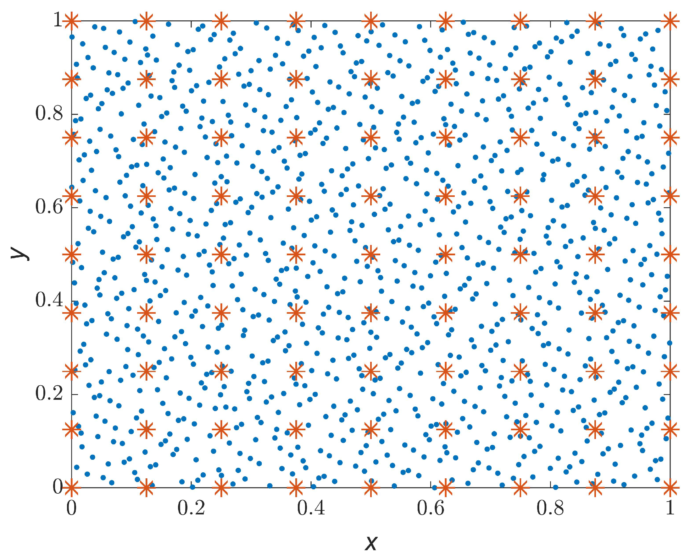In addition, a smaller set ${\mathcal{X}}_k=\{{\mathbf{x}}_{k_1},\dots ,{\mathbf{x}}_{k_m}\}$, with ${\mathbf{x}}_{k_j}=(x_{k_j},y_{k_j})\in {\mathrm{I}\mathrm{R}}^2$, of uniformly distributed data is given where every ${\mathbf{x}}_k$ is a center of a radial basis function in two dimensions. Both sets of data were provided on a CD supplied with the textbook. Figure 1 shows the positions of the data points together with the coordinates of the center points.

The problem is overdetermined with $n>m$ and the approximation is performed with the use of the least squares method. The approximation function (27) is built as a linear combination of radial basis functions with an addition of three linear polynomial terms. The chosen basic function for this problem is the thin-plate spline function, as it is given in (2). According to Fasshauer [4] (p. 71), the added polynomials are necessary in order for an interpolation problem using thin-plate splines to be well-posed. Nevertheless, an approximation problem is considered here and Fasshauer [4] (p. 170ff.) did not give a clear justification for the addition of the polynomials in this approximation problem.

Since the functions of this problem are not given explicitly in the aforementioned Section 19.4 of the textbook, the notation has been derived with the help of Section 6.2 (“Example: Reproduction of linear functions using Gaussian RBFs”) in Fasshauer [4] (p. 55ff.), the information given in Fasshauer [4] (p. 70ff.) and the source code given in Fasshauer [4] (p. 171). Therefore, the approximation function is formed as

$$s_i\left({\mathbf{x}}_i\right)=\sum _{i=1}^n{c}_{k_j}\left|\right|{\mathbf{x}}_i-{\mathbf{x}}_{k_j}{\left|\right|}_2^{2}log\left|\right|{\mathbf{x}}_i-{\mathbf{x}}_{k_j}{\left|\right|}_2+d_1+d_2{x}_i+d_3{y}_i$$

(27)

with $i=1,\dots ,n$ and $j=1,\dots ,m$. Now, to the number m of the unknown parameters $c_{k_j}$ are added three additional unknown parameters, namely $d_1,d_2,d_3$. This results in the total number of unknown parameters of the problem being $m+3$. However, the problem remains overdetermined with $n>m+3$.

Additionally to the function in (27), three constraint equations are considered in this approximation problem, given by

$$\begin{array}{cc}\hfill & \sum _{j=1}^m{c}_{k_j}=0,\hfill \\ \hfill & \sum _{j=1}^m{c}_{k_j}{x}_{k_j}=0,\hfill \\ \hfill & \sum _{j=1}^m{c}_{k_j}{y}_{k_j}=0,\hfill \end{array}$$

(28)

which, according to Fasshauer [4] (p. 58), are needed to ensure a unique solution. Here it must be noted that in Fasshauer [4] (p. 58), in this particular page of the textbook, an interpolation problem with added polynomial terms is considered, where $n=m$. Obviously, the three constraint equations are introduced because three additional unknown parameters are added to the function used for the interpolation. Since $n=m$, adding three unknown parameters leads to $n<m+3$, and the interpolation matrix would be singular because there would be a rank deficiency of three. In order to eliminate this rank deficiency, three constraint equations are added.

Back to the approximation problem described in Fasshauer [4] (p. 170ff.). The augmented system

$$\underset{{\mathbf{A}}_{\mathrm{ext}}}{\underbrace{\left[\begin{array}{cc}\mathbf{A}& \begin{array}{ccc}1& x_1& y_1\\ ⋮& ⋮& ⋮\\ 1& x_n& y_n\end{array}\\ \begin{array}{ccc}1& \cdots & 1\\ x_{k_1}& \cdots & x_{k_m}\\ y_{k_1}& \cdots & y_{k_m}\end{array}& \mathbf{O}\end{array}\right]}}\underset{\hat{\mathbf{X}}}{\underbrace{\left[\begin{array}{c}\begin{array}{c}{\hat{c}}_{k_1}\\ ⋮\\ {\hat{c}}_{k_m}\end{array}\\ \begin{array}{c}{\hat{d}}_1\\ {\hat{d}}_2\\ {\hat{d}}_3\end{array}\end{array}\right]}}=\underset{{\mathbf{L}}_{\mathrm{ext}}}{\underbrace{\left[\begin{array}{c}\begin{array}{c}{l}_1\\ ⋮\\ l_n\end{array}\\ \begin{array}{c}0\\ 0\\ 0\end{array}\end{array}\right]}},$$

(29)

derived from the code given in Fasshauer [4] (p. 171), needs to be solved. Here, the matrix

$${\mathbf{A}}_{n\times m}=\left[\begin{array}{ccc}\left|\right|{\mathbf{x}}_1-{\mathbf{x}}_{k_1}{\left|\right|}_2^{2}log\left|\right|{\mathbf{x}}_1-{\mathbf{x}}_{k_1}{\left|\right|}_2& \cdots & \left|\right|{\mathbf{x}}_1-{\mathbf{x}}_{k_m}{\left|\right|}_2^{2}log\left|\right|{\mathbf{x}}_1-{\mathbf{x}}_{k_m}{\left|\right|}_2\\ ⋮& \ddots & ⋮\\ \left|\right|{\mathbf{x}}_n-{\mathbf{x}}_{k_1}{\left|\right|}_2^{2}log\left|\right|{\mathbf{x}}_n-{\mathbf{x}}_{k_1}{\left|\right|}_2& \cdots & \left|\right|{\mathbf{x}}_n-{\mathbf{x}}_{k_m}{\left|\right|}_2^{2}log\left|\right|{\mathbf{x}}_n-{\mathbf{x}}_{k_m}{\left|\right|}_2\end{array}\right]$$

(30)

contains the radial basis functions. Since the coordinates of the center points ${\mathbf{x}}_{k_j},j=1,\dots ,m$ are different from each other,

$${\mathbf{x}}_{k_1}\ne {\mathbf{x}}_{k_2}\ne \dots \ne {\mathbf{x}}_{k_m}$$

(31)

applies. Thus, the columns of matrix $\mathbf{A}$ (30) are linearly independent and $\mathbf{A}$ has full (column) rank. The observations (or the noisy data) are denoted with $l_i,i=1,\dots ,n$ while the matrix $\mathbf{O}$ is a $3\times 3$ zero matrix.

In order for Fasshauer [4] (p. 170ff.) to solve this linear system of equations with the rectangular matrix ${\mathbf{A}}_{n\times m}$, he extended it, as shown in (29), by using the data points ${\mathbf{x}}_i=(x_i,y_i)$ in the right upper block of the augmented matrix and the center points ${\mathbf{x}}_{k_j}=(x_{k_j},y_{k_j})$ in the left lower block of the same matrix. Afterwards, he applied the built-in function of Matlab, known as “backslash operator” (∖ or mldivide), where according to the official documentation of Matlab, if the matrix $\mathbf{A}$ is rectangular, then $\mathbf{A}\backslash \mathbf{B}$ returns a least squares solution to the system of equations $\mathbf{A}\mathbf{x}=\mathbf{B}$.

For the solution of the example by Fasshauer [4] (p. 170ff.), the residuals

$$\mathbf{v}={\mathbf{A}}_{\mathrm{ext}}\hat{\mathbf{X}}-{\mathbf{L}}_{\mathrm{ext}},$$

(32)

cf. (14), and the objective function of the least squares method (10) were additionally calculated. The numerical result of the objective function is $\Omega =0.898200670635974$.

The condition number, see (23), of ${\mathbf{A}}_{\mathrm{ext}}$ which was used to obtain the solution, results in $k_2\left({\mathbf{A}}_{\mathrm{ext}}\right)=7184.37655737732$, while the condition number of the normal matrix

$$\mathbf{N}={\mathbf{A}}_{\mathrm{ext}}^{\mathrm{T}}{\mathbf{A}}_{\mathrm{ext}},$$

(33)

cf. (18) is $k_2\left(\mathbf{N}\right)=\mathrm{51,615,266.5155689}$. Furthermore, the normal matrix has full (maximum) rank with $\mathrm{rank}\left(\mathbf{N}\right)=84$, since this number is equal to the number of the unknown parameters of the problem, which is $81+3$. Additionally, the matrix ${\mathbf{A}}_{\mathrm{ext}}$ has full (column) rank with $\mathrm{rank}\left({\mathbf{A}}_{\mathrm{ext}}\right)=84$. Moreover, the eigenvalues of matrix $\mathbf{N}$ are all real and positive, which shows that the normal matrix is positive definite.

It should be mentioned that Fasshauer [4] (p. 170ff.) computes a least squares solution without explicitly building the normal matrix. Setting up this matrix and calculating the condition number is only presented here to compare it with the numerical results presented in Section 4 and Section 5.

For the example considered, Fasshauer [4] (p. 170ff.) did not explain how the set of the center points was selected. However, in Fasshauer [4] (p. 168), it is described that the approximation problem will have a unique solution if the rectangular matrix $\mathbf{A}$ has full rank. In particular, if the center points are chosen to form a subset of the data points, then the matrix $\mathbf{A}$ will have a square matrix $m\times m$, which will be non-singular.

The equations given in (28) were defined as constraint equations, which means that they are supposed to be rigorously fulfilled by the estimated unknown parameters ${\hat{c}}_k$. In fact, the results are the following

$$\begin{array}{cc}\hfill & \sum _{j=1}^m{\hat{c}}_{k_j}=-6.2096·{10}^{-4},\hfill \\ \hfill & \sum _{j=1}^m{\hat{c}}_{k_j}{x}_{k_j}=1.9300·{10}^{-4},\hfill \\ \hfill & \sum _{j=1}^m{\hat{c}}_{k_j}{y}_{k_j}=0.0010\hfill \end{array}$$

(34)

and it can be seen that all three equations are not equal to zero, as was requested in (28). This means that these equations are not defined as constraint equations but as additional equations to the function given in (27). This conclusion can also be derived from the extension of the matrix ${\mathbf{A}}_{\mathrm{ext}}$, where different points were used for each block of this matrix, as was explained previously. Moreover, the last three zero entries in the extended vector of the observations ${\mathbf{L}}_{\mathrm{ext}}$, given in (29), are introduced as “pseudo-observations” and hence residuals must be taken into account for these observations as well.

Therefore, the functions that describe this numerical example must be rewritten correctly as

$$\begin{array}{cc}\hfill s_i\left({\mathbf{x}}_i\right)=& \sum _{i=1}^n{c}_{k_j}\left|\right|{\mathbf{x}}_i-{\mathbf{x}}_{k_j}{\left|\right|}_2^{2}log\left|\right|{\mathbf{x}}_i-{\mathbf{x}}_{k_j}{\left|\right|}_2+d_1+d_2{x}_i+d_3{y}_i\hfill \\ \hfill 0=& \sum _{j=1}^m{c}_{k_j}\hfill \\ \hfill 0=& \sum _{j=1}^m{c}_{k_j}{x}_{k_j}\hfill \\ \hfill 0=& \sum _{j=1}^m{c}_{k_j}{y}_{k_j}\hfill \end{array}$$

(35)

where, according to (35), the observation equations can be formed as

$$\begin{array}{cc}\hfill l_i+v_i=& \sum _{i=1}^n{\hat{c}}_{k_j}\left|\right|{\mathbf{x}}_i-{\mathbf{x}}_{k_j}{\left|\right|}_2^{2}log\left|\right|{\mathbf{x}}_i-{\mathbf{x}}_{k_j}{\left|\right|}_2+{\hat{d}}_1+{\hat{d}}_2{x}_i+{\hat{d}}_3{y}_i\hfill \\ \hfill 0+v_{k_1}=& \sum _{j=1}^m{\hat{c}}_{k_j}\hfill \\ \hfill 0+v_{k_2}=& \sum _{j=1}^m{\hat{c}}_{k_j}{x}_{k_j}\hfill \\ \hfill 0+v_{k_3}=& \sum _{j=1}^m{\hat{c}}_{k_j}{y}_{k_j}\hfill \end{array}$$

(36)

with $l_i+v_i=s_i\left({\mathbf{x}}_i\right)$. Here, the zero values are additional observations, and residuals are considered for these observations as well. This, however, leads finally to the fact that the constraint equations are not strictly satisfied by the estimated parameters, see (34). This gives the motivation to develop a solution in which the constraint equations are rigorously satisfied, which will be shown in the following Section 4.

4. A Rigorous Constrained Solution of RBF Surface Approximation

The introduction of constraint equations in adjustment calculations can be traced far back in the geodetic literature, see, e.g., the textbook by Helmert [18] (p. 195ff.). Constraint equations are always introduced when a function of the estimated parameters must fulfil certain geometric or physical properties. In the case of a singular adjustment problem, d constraint equations can be introduced to eliminate a rank defect d of the design matrix. An example of this is the so-called free network adjustment, where the geodetic datum is fixed by introducing constraint equations for the coordinates to be determined.

For the approximation function (27), in which three additional unknown parameters were introduced by considering the polynomial terms, the design matrix $\mathbf{A}$ results, here, in

$${\mathbf{A}}_{n\times (m+3)}=\left[\begin{array}{cccccc}\left|\right|{\mathbf{x}}_1-{\mathbf{x}}_{k_1}{\left|\right|}_2^{2}log\left|\right|{\mathbf{x}}_1-{\mathbf{x}}_{k_1}{\left|\right|}_2& \cdots & \left|\right|{\mathbf{x}}_1-{\mathbf{x}}_{k_m}{\left|\right|}_2^{2}log\left|\right|{\mathbf{x}}_1-{\mathbf{x}}_{k_m}{\left|\right|}_2& 1& x_1& y_1\\ ⋮& \ddots & ⋮& ⋮& ⋮& ⋮\\ \left|\right|{\mathbf{x}}_n-{\mathbf{x}}_{k_1}{\left|\right|}_2^{2}log\left|\right|{\mathbf{x}}_n-{\mathbf{x}}_{k_1}{\left|\right|}_2& \cdots & \left|\right|{\mathbf{x}}_n-{\mathbf{x}}_{k_m}{\left|\right|}_2^{2}log\left|\right|{\mathbf{x}}_n-{\mathbf{x}}_{k_m}{\left|\right|}_2& 1& x_n& y_n\end{array}\right].$$

(37)

Despite the introduction of additional unknowns, the rank of this matrix is maximum with $\mathrm{rank}\left(\mathbf{A}\right)=84$. Thus, the problem can be solved without additional information, i.e., without the introduction of constraint equations. Furthermore, the problem remains overdetermined, although three additional unknown parameters were introduced.

Nevertheless, in the following it will be shown, by means of the numerical example from Section 3, how the three constraint equations (28) can be taken into account in a least squares adjustment problem in such a way that they are rigorously fulfilled by the estimated parameters.

Therefore, as shown in Section 2, the matrix $\mathbf{B}$ has to be set up, which contains the coefficients with which the unknown parameters in the constraint equations (28) are multiplied. This matrix results, in this case, in

$${\mathbf{B}}^{\mathrm{T}}=\left[\begin{array}{cccccc}1& \cdots & 1& 0& 0& 0\\ x_{k_1}& \cdots & x_{k_m}& 0& 0& 0\\ y_{k_1}& \cdots & y_{k_m}& 0& 0& 0\end{array}\right]$$

(38)

where zero values are included since in the constraint equations no polynomial terms are present.

With the design matrix $\mathbf{A}$ in (37), the normal matrix $\mathbf{N}$ according to (18) can be formed, and thus the extended normal equation system

$$\underset{{\mathbf{N}}_{\mathrm{ext}}}{\underbrace{\left[\begin{array}{cc}\mathbf{N}& \begin{array}{ccc}1& x_{k_1}& y_{k_1}\\ ⋮& ⋮& ⋮\\ 1& x_{k_m}& y_{k_m}\\ 0& 0& 0\\ 0& 0& 0\\ 0& 0& 0\end{array}\\ \begin{array}{cccccc}1& \cdots & 1& 0& 0& 0\\ x_{k_1}& \cdots & x_{k_m}& 0& 0& 0\\ y_{k_1}& \cdots & y_{k_m}& 0& 0& 0\end{array}& \mathbf{O}\end{array}\right]}}\underset{{\hat{\mathbf{X}}}_{\mathrm{ext}}}{\underbrace{\left[\begin{array}{c}\begin{array}{c}{\hat{c}}_{k_1}\\ ⋮\\ {\hat{c}}_{k_m}\end{array}\\ \begin{array}{c}{\hat{d}}_1\\ {\hat{d}}_2\\ {\hat{d}}_3\end{array}\\ \begin{array}{c}{k}_1\\ k_2\\ k_3\end{array}\end{array}\right]}}=\underset{{\mathbf{n}}_{\mathrm{ext}}}{\underbrace{\left[\begin{array}{c}\begin{array}{c}\mathbf{n}\end{array}\\ \begin{array}{c}0\\ 0\\ 0\end{array}\end{array}\right]}},$$

(39)

cf. (25) can be set up. The right hand side vector of the system $\mathbf{n}$ is calculated as in (19). Since the three constraint equations given in (28) must each yield the value zero, a zero vector of the dimension $3\times 1$ is appended. The extended vector ${\hat{\mathbf{X}}}_{\mathrm{ext}}$ contains the coefficients of the unknown parameters, the additional unknown parameters of the polynomials and the Lagrange multipliers $k_1,k_2,k_3$. The residuals

$$\mathbf{v}=\mathbf{A}{\hat{\mathbf{X}}}_{\mathrm{ext}(1:m+3)}-\mathbf{L}$$

(40)

can be computed according to (14). The numerical result of the objective function (10) is $\Omega =0.898202120259992$, which is slightly larger (the difference starts in the sixth decimal place) than the numerical result of the objective function given in the previous Section 3.

Inserting the estimated parameters into the constraint equations, the following results

$$\begin{array}{cc}\hfill & \sum _{j=1}^m{\hat{c}}_{k_j}=-7.5495·{10}^{-15},\hfill \\ \hfill & \sum _{j=1}^m{\hat{c}}_{k_j}{x}_{k_j}=-3.5527·{10}^{-15},\hfill \\ \hfill & \sum _{j=1}^m{\hat{c}}_{k_j}{y}_{k_j}=-5.3291·{10}^{-15}\hfill \end{array}$$

(41)

are obtained, and it can be stated that within the range of the machine precision (in this case double precision), these yield the value zero as a result. Thus, the constraint equations are rigorously fulfilled by the presented adjustment technique.

Additionally, the design matrix $\mathbf{A}$, the normal matrix $\mathbf{N}$ and the extended normal matrix ${\mathbf{N}}_{\mathrm{ext}}$ also have, in this case, full rank. This, according to the theory in Section 2, means that the solution is unique under the consideration of the constraint equations. Finally, the condition number of the design matrix is $k_2\left(\mathbf{A}\right)=8185.25268575357$ and the condition number of the extended normal matrix is $k_2\left({\mathbf{N}}_{\mathrm{ext}}\right)=50,687,555.5898314$.

Obviously, the condition number of the extended normal matrix is not much better than the condition number of the normal matrix given in Section 3. Furthermore, the calculation of the eigenvalues of the extended normal matrix ${\mathbf{N}}_{\mathrm{ext}}$ shows that all eigenvalues are real, of which three values are negative and the others are positive. This is expected since three constraint equations were introduced into this problem. This phenomenon, that the number of negative eigenvalues corresponds to the number of constraint equations introduced, can also be found in typical geodetic problems such as free network adjustment.

5. RBF Surface Approximation without Polynomial Terms

In Section 3 and Section 4, the RBF surface approximation problem was presented considering three linear polynomial terms. As already mentioned in the introduction of this article, this addition of polynomial terms along with thin-plate spline functions has been widely used in the RBF literature, mainly for interpolation, and for almost any application. Fasshauer [4] (p. 55) explained that in some cases it is desirable that the interpolant exactly reproduces certain types of functions, e.g., constant or linear. Particularly in applications, he continued, related to partial differential equations (finite element methods), or in specific engineering applications (exact calculation of constant stress and strain), the reproduction of these simple linear polynomials is a necessity.

This leads to the important conclusion that polynomial terms are added when the application has certain requirements and it is motivated solely by the user’s intention to obtain a solution with certain properties. This conclusion can also be drawn from the article by Duchon [8] where he was interested in an interpolating surface as close to a plane as possible. Similarly, Hardy [10] added polynomial terms with multiquadric functions to the interpolation function to obtain an interpolating surface where surface tangents coincide at specified points. Finally, there seem to be (infinite dimensional) problems in physics where what is interpolated or approximated has almost a planar form with some small deviations. For all these applications, the added polynomial terms can be very useful.

However, the thin-plate spline function can be used as a basis for an interpolation or an approximation problem with the RBF approach without the polynomials. In particular, for the geodetic application of point cloud modelling, the data (geodetic) do not have the characteristics of the aforementioned problems. Hence, there is no need for these polynomials. Moreover, due to the high point density of the point clouds, the added polynomials would not significantly smooth the approximated surface.

In this section, the same numerical example will be considered, as in Section 3, but in this case, no polynomials will be used. Therefore, the function without additional polynomial terms reads

$$s_i\left({\mathbf{x}}_i\right)=\sum _{i=1}^n{c}_{k_j}\left|\right|{\mathbf{x}}_i-{\mathbf{x}}_{k_j}{\left|\right|}_2^{2}log\left|\right|{\mathbf{x}}_i-{\mathbf{x}}_{k_j}{\left|\right|}_2.$$

(42)

In the overdetermined case, this function can only be fulfilled by the (theoretical) true values for the measurements ${\tilde{l}}_i$ and the unknown parameters ${\tilde{c}}_{k_j}$, and the functional model is written

$${\tilde{l}}_i=\sum _{i=1}^n{\tilde{c}}_{k_j}\left|\right|{\mathbf{x}}_i-{\mathbf{x}}_{k_j}{\left|\right|}_2^{2}log\left|\right|{\mathbf{x}}_i-{\mathbf{x}}_{k_j}{\left|\right|}_2.$$

(43)

Since the true values are, of course, not known in practical applications, a solution according to the method of least squares is to be determined, for which the observation equations

$$l_i+v_i=\sum _{i=1}^n{\hat{c}}_{k_j}\left|\right|{\mathbf{x}}_i-{\mathbf{x}}_{k_j}{\left|\right|}_2^{2}log\left|\right|{\mathbf{x}}_i-{\mathbf{x}}_{k_j}{\left|\right|}_2$$

(44)

are set up, where $l_i,i=1,\dots ,n$ are the measurements and $v_i,i=1,\dots ,n$ are the residuals.

The design matrix $\mathbf{A}$, which contains the coefficients associated with the unknown parameters ${\hat{c}}_{k_j}$, is calculated as already shown in (30). The normal equations given in (17) are built with the normal matrix $\mathbf{N}$ (18). The solution of the normal equations is derived (20).

The numerical result of the objective function (10) is $\Omega =0.897883029539522$, which is smaller (the difference starts in the third decimal place) than the numerical result of the objective function from the techniques in Section 3 and Section 4. The normal matrix $\mathbf{N}$ and the design matrix $\mathbf{A}$ both also have in this case full rank, which is equal to the number of the unknown parameters $m=81$, and thus the solution is unique.

The condition number of the design matrix is $k_2\left(\mathbf{A}\right)=4741.09857980940$ and the condition number of the normal matrix is $k_2\left(\mathbf{N}\right)=22,478,015.7415776$. These condition numbers appear smaller compared to the condition numbers given in the previous two sections but they still have the same order of magnitude as the others. Furthermore, the eigenvalues of the normal matrix are all real and positive, thus the normal matrix is positive definite. 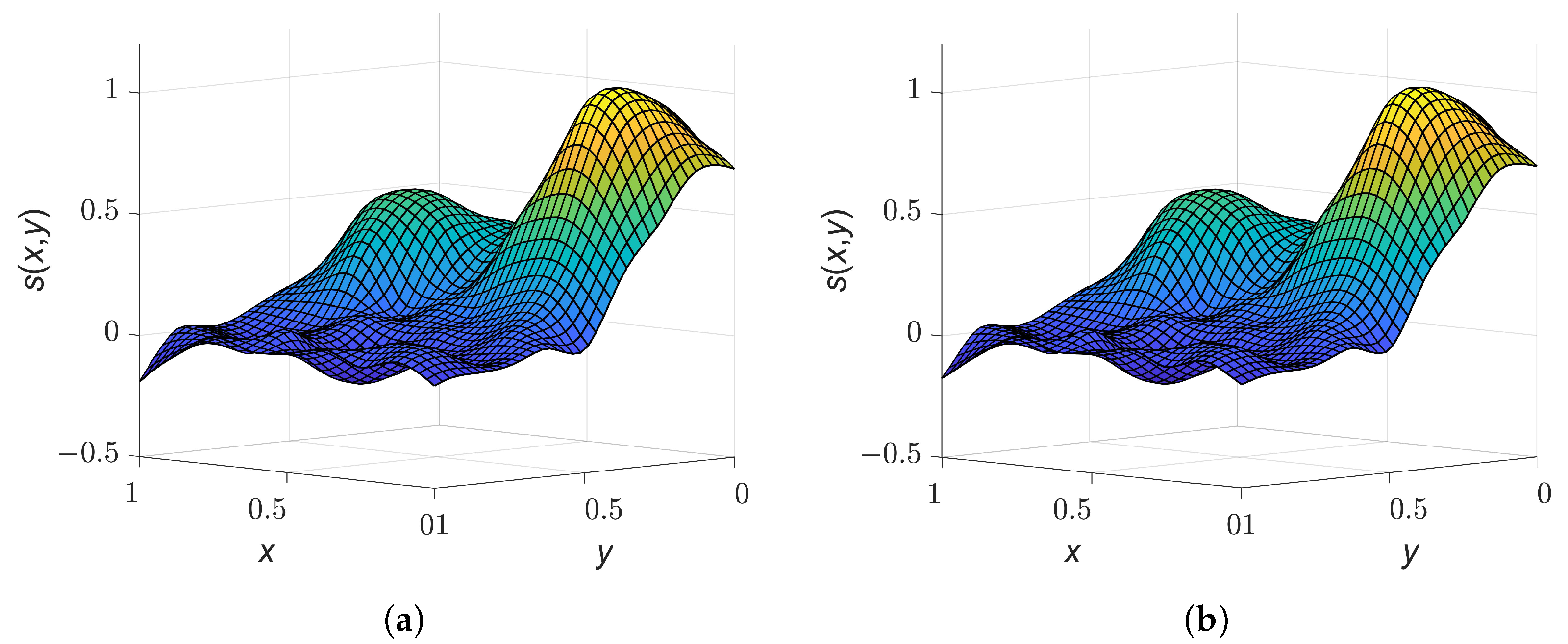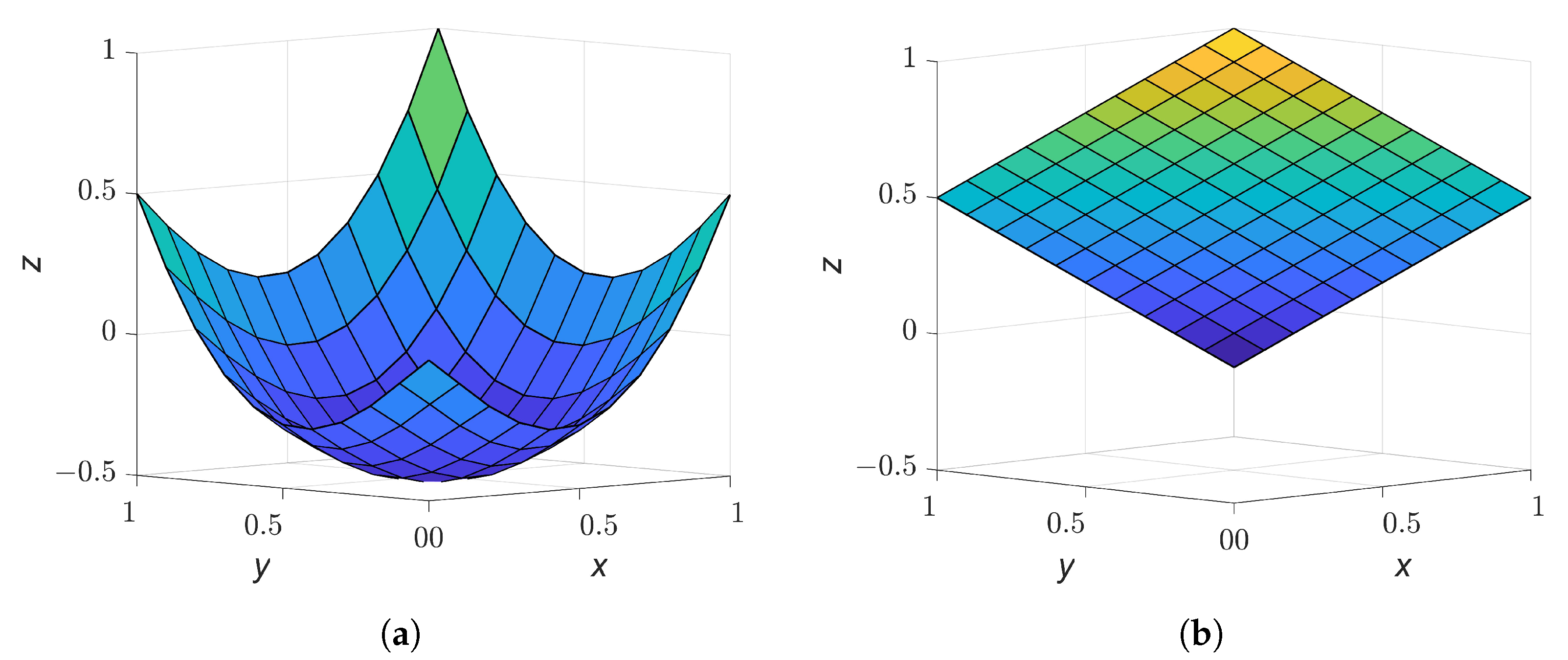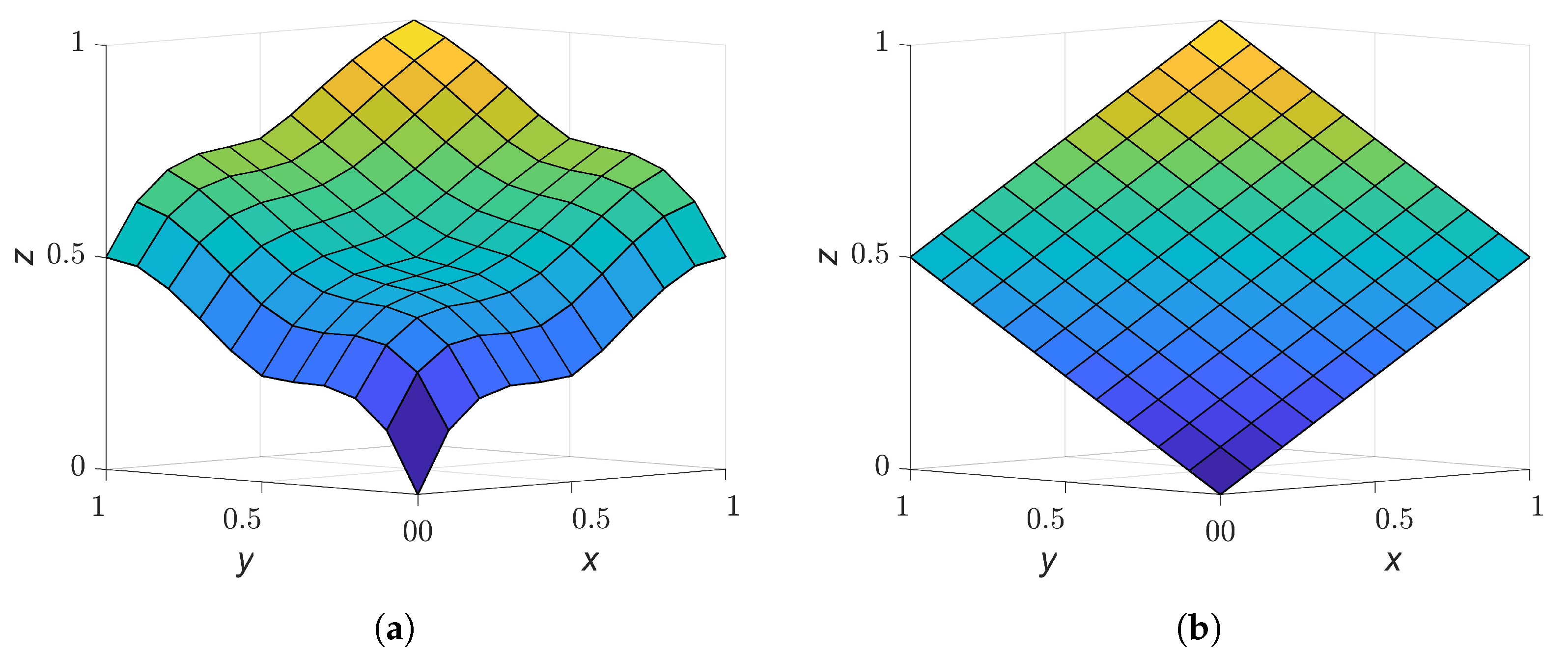The following Figure 2a shows the original (exact) surface derived from the Franke’s function given in Section 3. Figure 2b shows the resulting approximated surface calculated in this section.

6. Comparison and Discussion of the Investigated Techniques for Surface Approximation with Thin-Plate Splines

In Section 3, Section 4 and Section 5, the same numerical example was computed in each surface approximation technique. For this numerical example, the measurements were “created” using Franke’s function. Thus, the original surface is known, see Figure 2a, and the numerical differences between the values of the original surface and the values of the approximated surfaces can be calculated. Therefore, the absolute error

$$e_i=|s_i\left({\mathbf{\xi }}_i\right)-f_i\left({\mathbf{\xi }}_i\right)|,i=1,\dots ,M$$

(45)

is computed, with $s_i\left({\mathbf{\xi }}_i\right)$ points of the approximated surface and $f_i\left({\mathbf{\xi }}_i\right)$ points of the original surface. The points ${\mathbf{\xi }}_i$ are equally spaced points, here of $40\times 40$, covering the $[0,1]\times [0,1]$ square in two dimensions, and they are called evaluation points. Figure 3 illustrates the absolute errors $e_i$ for the different solutions from Section 3, Section 4 and Section 5.

Additionally,

Table 2. Maximum absolute error.

Solutions	$max\mathit{e}$
Solution of Section 3	$0.0458118752483207$
Solution of Section 4	$0.0458077776895431$
Solution of Section 5	$0.0438325527609283$

contains the maximum value of the absolute error from the three solutions.

Besides the absolute error, the Root-Mean-Square error (RMS–error) can be computed as well. According to Fasshauer [4] (p. 10), the RMS–error is given by

$$\mathit{RMS}--\mathit{error}=\frac{1}{\sqrt{M}}\left|\right|s_i\left({\mathbf{\xi }}_i\right)-f_i\left({\mathbf{\xi }}_i\right){\left|\right|}_2,i=1,\dots ,M.$$

(46)

Table 3. RMS–error.

Solutions	$\mathit{RMS}–\mathit{error}$
Solution of Section 3	$0.00940700731481119$
Solution of Section 4	$0.00940714649245884$
Solution of Section 5	$0.00931918546911314$

contains the RMS–error for the solutions given in the previous three sections.

From Table 2 and Table 3 it can be seen that the solution presented in Section 5 gives the smallest values for both the maximum absolute error and the RMS–error. The value of the maximum absolute error of the solution presented in Section 4 is slightly smaller (differs in the fifth digit after the comma) than the value of this error from the solution in Section 3, see Table 2. On the contrary, the value of the RMS–error of the solution in Section 3 is slightly smaller (differs in the seventh digit after the comma) than the value of this error from the solution in Section 4, see Table 3.

Equivalent to the RMS–error, the numerical value of the objective function of the least squares method, see

Table 4. Numerical result of $\Omega$ for each solution.

Solutions	$\mathit{\Omega }$
Solution of Section 3	$0.898200670635974$
Solution of Section 4	$0.898202120259992$
Solution of Section 5	$0.897883029539522$

, can be used as a measure of the goodness of fit.

As for the RMS–error, the smallest value of the objective function results from the solution from Section 5 where no polynomials and constraint equations were introduced into the problem.

In addition, condition numbers for the design matrices and the normal matrices were given for the solution of each section, which are compiled in

Table 5. Condition numbers of $\mathbf{A}$ and ${\mathbf{A}}_{\mathrm{ext}}$.

Solutions	Design Matrix	${\mathit{k}}_2(·)$
Solution of Section 3	${\mathbf{A}}_{\mathrm{ext}(1092\times 84)}$	$7184.37655737732=7.1844·{10}^3$
Solution of Section 4	${\mathbf{A}}_{(1089\times 84)}$	$8185.25268575357=8.1853·{10}^3$
Solution of Section 5	${\mathbf{A}}_{(1089\times 81)}$	$4741.09857980940=4.7411·{10}^3$

and

Table 6. Condition numbers of $\mathbf{N}$ and ${\mathbf{N}}_{\mathrm{ext}}$.

Solutions	Normal Matrix	${\mathit{k}}_2(·)$
Solution of Section 3	${\mathbf{N}}_{(84\times 84)}$	$51,615,266.5155689=5.1615·{10}^7$
Solution of Section 4	${\mathbf{N}}_{\mathrm{ext}(84\times 84)}$	$50,687,555.5898314=5.0688·{10}^7$
Solution of Section 5	${\mathbf{N}}_{(81\times 81)}$	$22,478,015.7415776=2.2478·{10}^7$

.

The condition numbers of the design matrices in Table 5 are similar in numerical quantity, as they are of the same order of magnitude, ${10}^3$. According to Trefethen and Bau [17] (p. 95), if $\mathbf{A}$ is ill-conditioned, one always expects to “lose ${log}_{10}k\left(\mathbf{A}\right)$ digits” in computing the solution. For the numerical examples in Section 3, Section 4 and Section 5, the matrices of all the cases are mildly ill-conditioned and ${log}_{10}{k}_2\left(\mathbf{A}\right)=4$ for every case. Alternatively, working with double precision in Matlab with 64 bits, the machine epsilon is $2^{-52}\approx {10}^{-16}$, which that means double precision numbers can be accurate to about 16 decimal places. Multiplying the machine epsilon with the condition numbers in Table 5, the result for every case is ${10}^{-12}$. This means that at least 12 digits in the solutions of the previous sections are correct. Hence, 4 digits must be ignored. Similar conclusions can also be drawn for the condition numbers in Table 6 since the condition number of the normal matrix (or the extended normal matrix) computed as $k_2\left({\mathbf{A}}^{\mathrm{T}}\mathbf{A}\right)$ is equal to the square of the condition number $k_2\left(\mathbf{A}\right)$.

Considering the fact that erroneous data (measurements) are involved in the approximation problems in Section 3, Section 4 and Section 5, the linear system of equations, in each case, with respect to the solution, presents low sensitivity. That is, the solution can be “trusted” up to 12 decimal places for every case. Moreover, the introduction of polynomial terms and constraint equations into the problem showed no improvement with respect to the sensitivity of the computation process. This means that the condition number of the design matrices in Section 3 and Section 4 was not of a smaller order of magnitude than the condition number of the design matrix in Section 5.

Furthermore, the errors in Table 2 and Table 3, and the objective functions in Table 4, showed that the solution from Section 5 provides a better approximation in terms of smallest deviations than the solutions from Section 3 and Section 4. It should be noted that the solution in Section 5 was determined with a different approximation function than the solutions in Section 3 and Section 4, as no polynomial terms and constraint equations were introduced. By adding polynomials, see (27), or by considering additional equations, see (35), modification of the mathematical function(s) of the problem is made. This leads to the solution of a different problem, since the mathematical function(s) chosen must describe the current problem as well as possible.

The investigations presented up to this point were carried out for a noise level of $3\%$ for the observations. In order to determine how a larger noise level affects the surface approximation with and without polynomials and constraint equations, the previously described investigations were carried out with a noise level of $10\%$. A visualisation of the approximated surfaces based on the techniques in Section 4 and Section 5 is shown in Figure 4.

Obviously, there are no significant differences between the results from both solution approaches. This is also reflected in the a posteriori parameters in

Table 7. A posteriori parameters of the approximations with and without consideration of polynomials and constraint equations for a dense point cloud.

	Approximation without Polynomials and Constraints	Approximation with Polynomials and Constraints
$maxe$	$0.190894095935541$	$0.173790735048742$
$\mathit{RMS}–\mathit{error}$	$0.0288347260922599$	$0.0285738186155563$
$\Omega$	$10.1849862842421$	$10.1856091103718$

.

It can be observed that all values show no significant deviations. Therefore, it can be concluded that even for data sets with a higher noise level, the introduction of polynomial terms and the corresponding constraints does not lead to a significant smoothing of the approximated surface for dense point clouds.

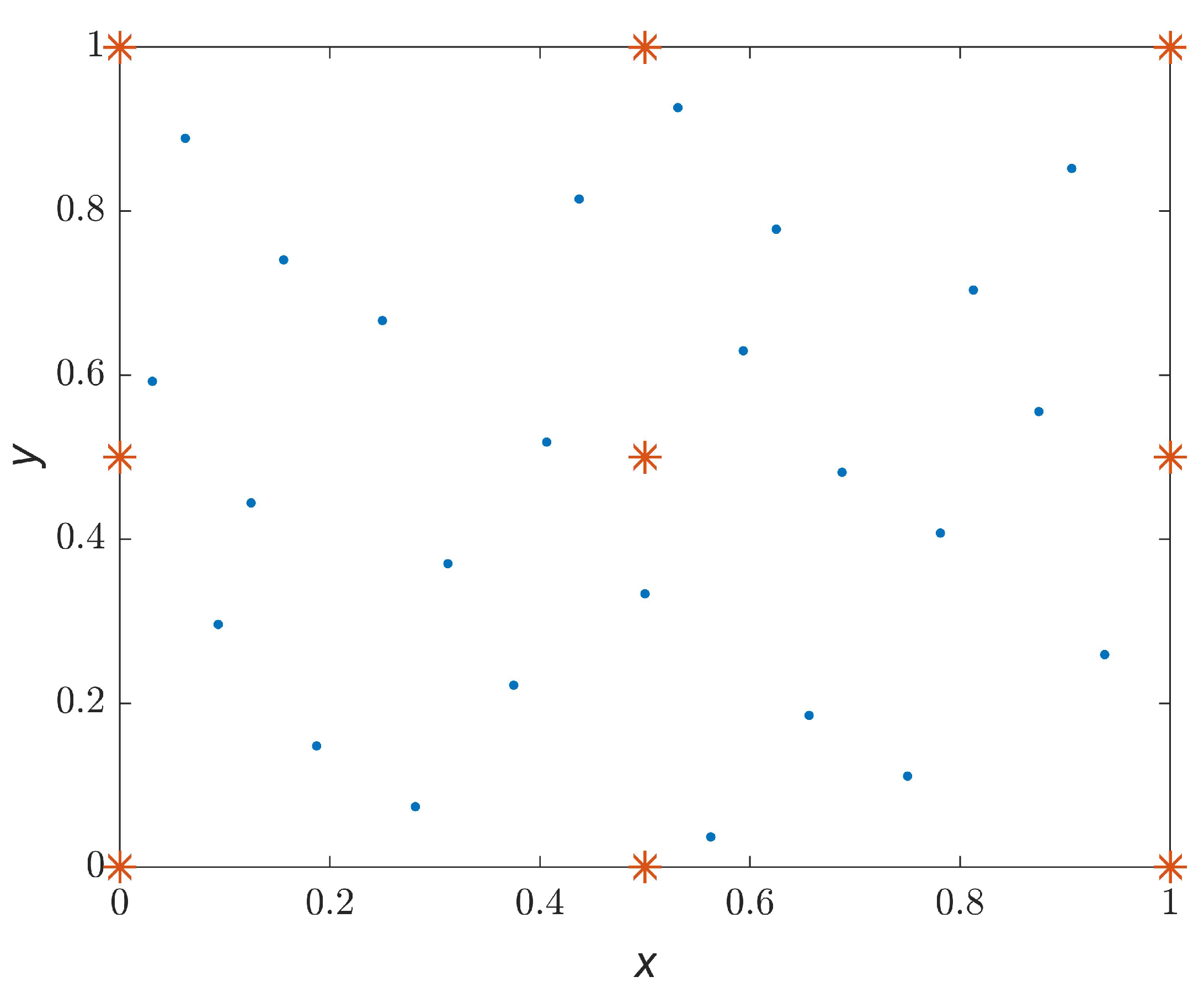
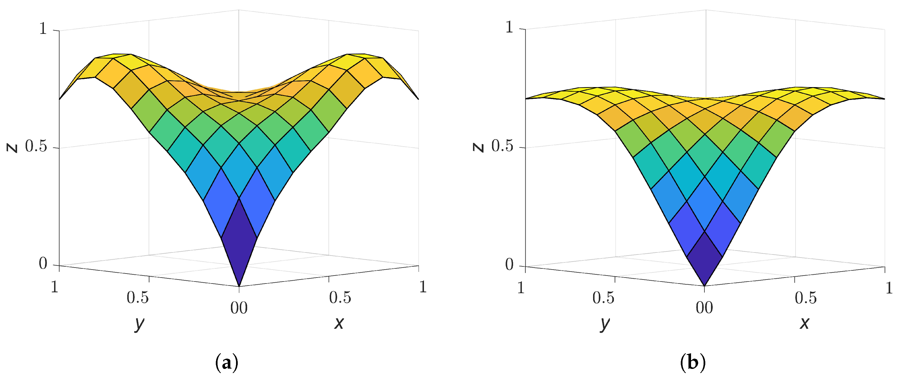
Since these findings are so far based on the evaluation of only one data set representing a dense point cloud, another numerical example will be considered in the following. Using the function

$$f(x,y)=ysin\left(2\mathsf{\pi }x\right)+xcos\left(2\mathsf{\pi }y\right)$$

(47)

the “measurements” (noisy data) are created taking into account a set $\mathcal{X}=\{{\mathbf{x}}_1,\dots ,{\mathbf{x}}_n\}$, with ${\mathbf{x}}_i=(x_i,y_i)\in {\mathrm{I}\mathrm{R}}^2$, to which $10\%$ of normally distributed random noise is added. The number of data points is 25, thus resulting in a sparse point cloud of a more curved surface. Moreover, a set ${\mathcal{X}}_k=\{{\mathbf{x}}_{k_1},\dots ,{\mathbf{x}}_{k_m}\}$, with ${\mathbf{x}}_{k_j}=(x_{k_j},y_{k_j})\in {\mathrm{I}\mathrm{R}}^2$, of uniformly distributed center points, is given. The number of center points is 9. The files with the data points and the center points are taken from the CD in the appendix of the textbook by Fasshauer [4]. 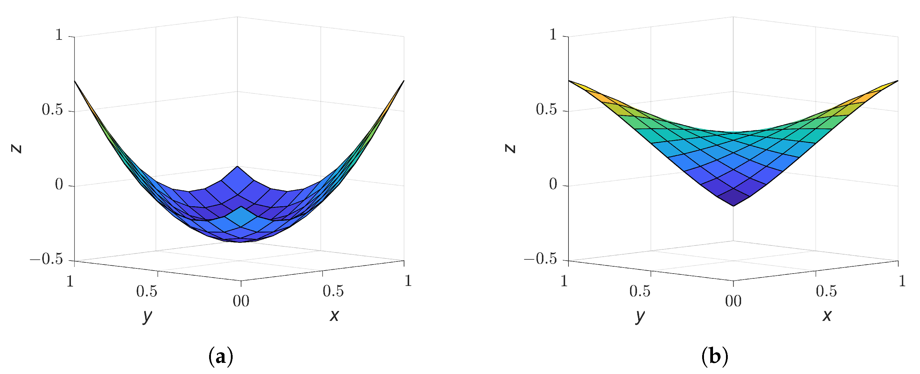Figure 5 shows the positions of the data points together with the coordinates of the center points.

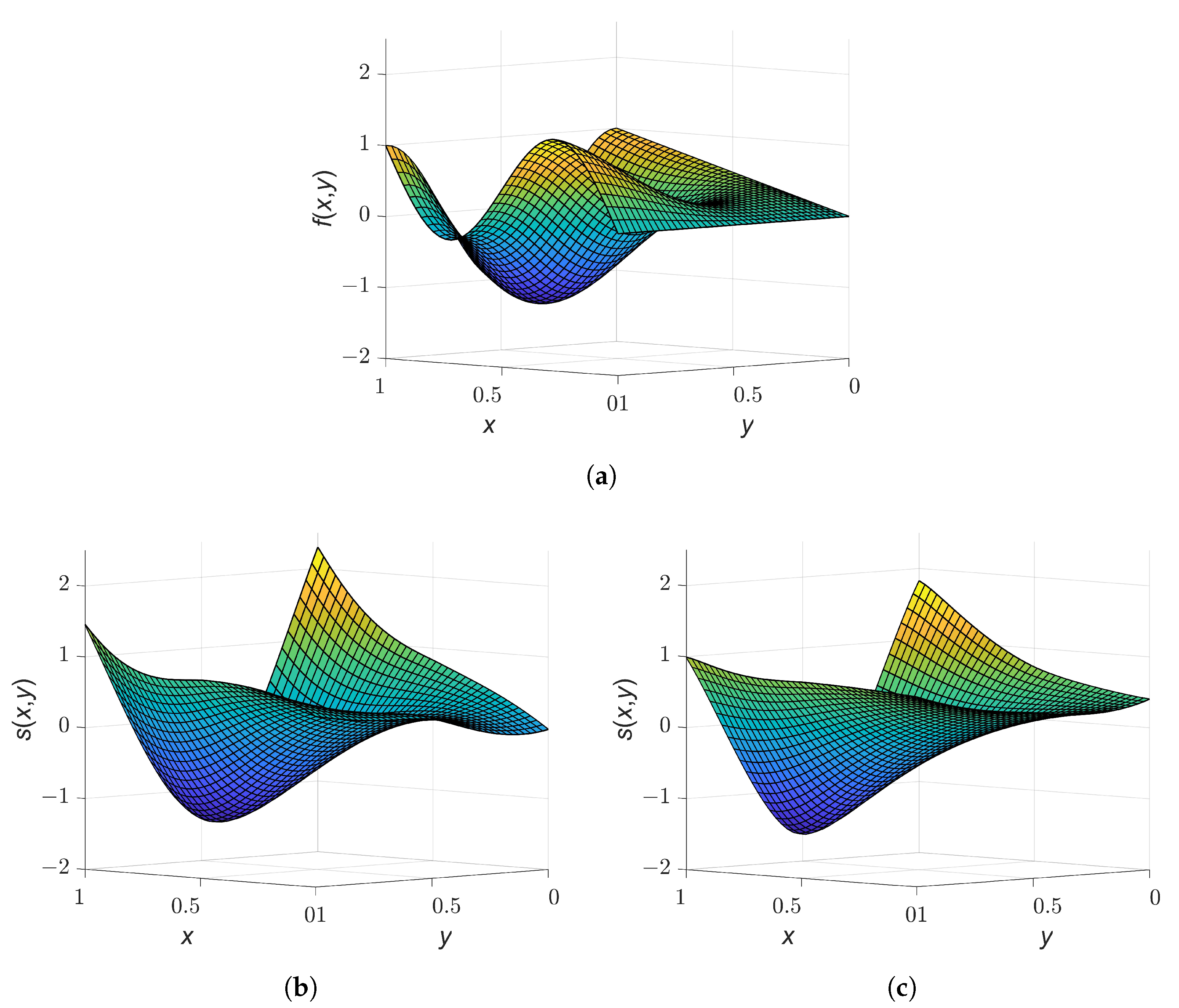
The original surface and the approximated ones with and without polynomials and constraint equations are shown in Figure 6.

In contrast to the previous example, it can already be recognised visually that the surface approximated using polynomials and constraint equations is smoother than the one without taking them into account. However, a stronger smoothing of the approximated surface immediately leads to the fact that it no longer fits the original data set so well. This can also be observed in the comparison of the a posteriori parameters in

Table 8. A posteriori parameters of the approximations with and without consideration of polynomials and constraint equations for a sparse point cloud.

	Approximation without Polynomials and Constraints	Approximation with Polynomials and Constraints
$maxe$	$1.30113223069638$	$1.04351806610705$
$\mathit{RMS}–\mathit{error}$	$0.266707361720968$	$0.289896867588036$
$\Omega$	$0.578752413858867$	$0.814187380865068$

. Since the smoother surface leads to larger residuals, the value $\Omega$, for example, is significantly larger than the value for an approximation without polynomials and the corresponding constraint equations.

Regarding applications with very high noise levels in the input data, in addition to the investigations with noise levels $3\%$ and $10\%$, the previously described calculations are carried out with higher noise levels of up to $80\%$. Figure 7 shows the value of the objective function $\Omega$ for different noise levels.

Firstly, it can be stated that the value of the objective function (10) increases with increasing noise level, because the residuals become larger. Comparing the solutions with and without consideration of polynomials and corresponding constraint equations, it can be observed that up to a noise level of $50\%$, the value of the objective function $\Omega$ is larger with consideration of polynomials and constraint equations than without their consideration. This indicates a stronger smoothing of the approximated surface, which then results in larger residuals. At a noise level of $60\%$, the solution with polynomials and constraint equations yields a slightly lower value of the objective function, above which the situation described previously is again apparent.

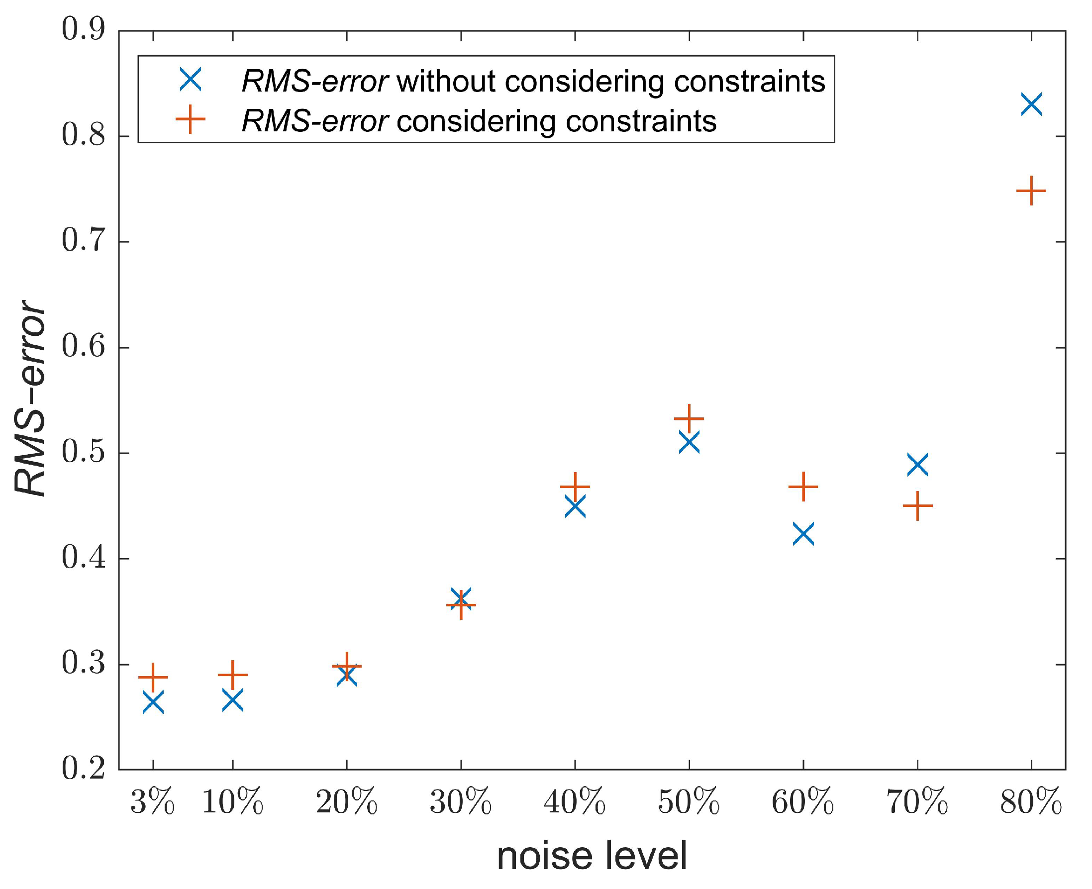
To evaluate how the solutions at different noise levels for the observations affect the shape of the approximated surface, the RMS–error (46) can be used, see Figure 8, as it describes the deviation of the approximated surface from the original one given by (47).

It can be observed that for a noise level up to $20\%$, the resulting surfaces are almost identical, both for the solutions with and without polynomials and constraint equations. For noise levels from $30\%$ to $70\%$, there is still a good agreement with the original surface, whereas at $80\%$, a larger deviation from it can be observed. From a noise level of $70\%$ onwards, it can be seen in the investigated example that the solution with polynomials and constraint equations leads to a lower RMS–error. This indicates that the polynomials and the constraint equations can have a positive effect on the resulting approximated surface for sparse point clouds with a very high noise level.

The numerical investigations in this section have shown that the consideration of polynomials and the associated constraint equations in the case of dense point clouds have no significant influence on the approximated surface compared to a solution without polynomials. Neighbouring points are so close to each other that the polynomials do not have a significant smoothing effect on the approximated surface. For sparse point clouds, on the other hand, a smoothing effect could be observed. It should be noted, however, that in this case, larger residuals result, since the approximated surface no longer fits the given data points so well. Based on the RMS–error it could be observed that the approximated surface agrees very well with the original surface known in the numerical example up to a noise level of $20\%$, both with and without consideration of polynomials and constraint equations. The influence of the polynomial terms on the resulting surface is further investigated in the following section by means of the interpolation of sparse point clouds.

7. Comparison of Interpolation Problems

Based on the interpolation technique that Hardy [10] introduced, eight interpolation problems are considered here with very few discrete data points. Four different sets of points $({\mathbf{x}}_i,z_i),i=1,\dots ,n$, with ${\mathbf{x}}_i=(x_i,y_i)\in {\mathrm{I}\mathrm{R}}^2$ and $z_i\in \mathrm{I}\mathrm{R}$, are given. For the interpolation process, the center points ${\mathbf{x}}_{k_i},i=1,\dots ,n$ with ${\mathbf{x}}_{k_i}=(x_{k_i},y_{k_i})\in {\mathrm{I}\mathrm{R}}^2$, of each problem, are equal and identical to the data sites ${\mathbf{x}}_i,i=1,\dots ,n$.

For every set of given points, the interpolation problem with thin-plate splines is solved twice. First is case (a), by using the function given in (42) where no added polynomials or constraint equations are considered, and then is case (b), by using the function given in (27) where three linear polynomials and three constraint equations given in (28) are involved. This results in eight solutions for the four given data sets. For each problem, the interpolation condition is defined as

$$s_i\left({\mathbf{x}}_i\right)=z_i.$$

(48)

For case (a) the system of linear equations has the form

$$\mathbf{A}\mathbf{X}=\mathbf{Z}$$

(49)

where $\mathbf{A}$ is a square matrix of dimension $n\times n$ and it is set up as in (30). The vector $\mathbf{X}={[c_{k_1}{c}_{k_2}...c_{k_n}]}^{\mathrm{T}}$ contains the unknown parameters and $\mathbf{Z}={[z_1{z}_2...z_n]}^{\mathrm{T}}$.

For case (b), the system of linear equations with additional constraint equations

$$\underset{{\mathbf{A}}_{\mathrm{ext}}}{\underbrace{\left[\begin{array}{cc}\mathbf{A}& \begin{array}{ccc}1& x_{k_1}& y_{k_1}\\ ⋮& ⋮& ⋮\\ 1& x_{k_n}& y_{k_n}\end{array}\\ \begin{array}{ccc}1& \cdots & 1\\ x_{k_1}& \cdots & x_{k_n}\\ y_{k_1}& \cdots & y_{k_n}\end{array}& \mathbf{O}\end{array}\right]}}\underset{{\mathbf{X}}_{\mathrm{ext}}}{\underbrace{\left[\begin{array}{c}\begin{array}{c}{c}_{k_1}\\ ⋮\\ c_{k_n}\end{array}\\ \begin{array}{c}{d}_1\\ d_2\\ d_3\end{array}\end{array}\right]}}=\underset{{\mathbf{Z}}_{\mathrm{ext}}}{\underbrace{\left[\begin{array}{c}\begin{array}{c}{z}_1\\ ⋮\\ z_n\end{array}\\ \begin{array}{c}0\\ 0\\ 0\end{array}\end{array}\right]}}$$

(50)

is built with $\mathbf{A}$ to be set up as shown in (30) while $\mathbf{O}$ is a $3\times 3$ zero matrix. Also, in this case, ${\mathbf{A}}_{\mathrm{ext}}$ is a square matrix of dimension $(n+3)\times (n+3)$. The vector ${\mathbf{X}}_{\mathrm{ext}}$ contains the unknown parameters associated with the radial basis functions and the unknown parameters of the polynomials, see (27).

Table 9. Data set no. 1.

x	y	z
0.0	1.0	0.5
1.0	1.0	1.0
0.0	0.0	0.0
1.0	0.0	0.5

,

Table 10. Data set no. 2.

x	y	z
0.00000	1.00000	0.70711
1.00000	1.00000	0.00000
0.00000	0.00000	0.00000
1.00000	0.00000	0.70711

,

Table 11. Data set no. 3.

x	y	z
0.00	1.00	0.50
0.50	1.00	0.75
1.00	1.00	1.00
0.00	0.50	0.25
0.50	0.50	0.50
1.00	0.50	0.75
0.00	0.00	0.00
0.50	0.00	0.25
1.00	0.00	0.50

and

Table 12. Data set no. 4.

x	y	z
0.00000	1.00000	0.70711
0.50000	1.00000	0.61237
1.00000	1.00000	0.00000
0.00000	0.50000	0.61237
0.50000	0.50000	0.70711
1.00000	0.50000	0.61237
0.00000	0.00000	0.00000
0.50000	0.00000	0.61237
1.00000	0.00000	0.70711

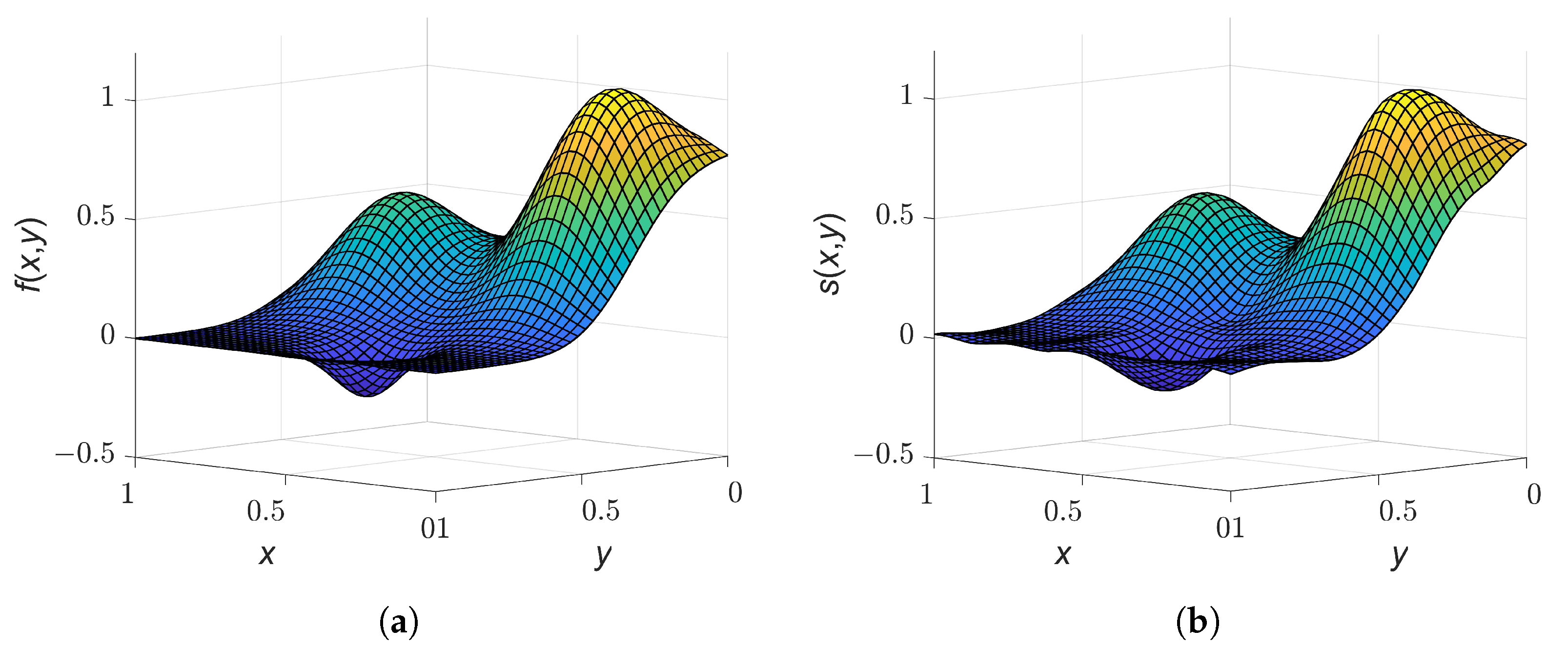
show the given data sets for each numerical example. Figure 9, Figure 10, Figure 11 and Figure 12 present the interpolated surfaces obtained from both cases where in case (a) no polynomials were added to the interpolation function and no constraint equations were introduced, and in case (b) three polynomials were added to the interpolation function and three constraint equations were taken into account.

In Figure 9, Figure 10, Figure 11 and Figure 12, the same phenomenon can be observed for each interpolation problem. This is, when the interpolation was performed without additional polynomials in the interpolation function and without constraint equations, see case (a), the interpolated surface has larger curvatures. On the other hand, when the interpolation was performed with additional polynomials and constraint equations, see case (b), the interpolated surface is smoother, and in two solutions, even has the shape of a plane, see Figure 9b and Figure 11b.

The goal of determining an interpolated surface that is as smooth as possible was probably the motivation for Duchon [8]’s investigations. Hardy [10] did not explicitly look for a surface that was as smooth as possible, but was rather interested in the surface tangents to coincide at specified points. Using numerical examples, it could be shown that the addition of polynomials and constraint equations can influence the smoothness of the interpolated surface, in some cases considerably, depending on the data set used.

Furthermore, it can be determined from the numerical investigations that the interpolation matrices $\mathbf{A}$ in case (a) (without consideration of polynomials and constraint equations) as well as ${\mathbf{A}}_{\mathrm{ext}}$ in case (b) (with consideration of polynomials and constraint equations) have full rank in each case. The condition numbers (23) of the matrices $\mathbf{A}$ and ${\mathbf{A}}_{\mathrm{ext}}$ are listed in

Table 13. Condition numbers of matrix $\mathbf{A}$ for the problems of case (a).

Data Set	Interpolation Matrix	${\mathit{k}}_2\left(\mathbf{A}\right)$
no. 1	${\mathbf{A}}_{(4\times 4)}$	1
no. 2	${\mathbf{A}}_{(4\times 4)}$	1
no. 3	${\mathbf{A}}_{(9\times 9)}$	8.02785191206729
no. 4	${\mathbf{A}}_{(9\times 9)}$	8.02785191206729

and

Table 14. Condition numbers of matrix ${\mathbf{A}}_{\mathrm{ext}}$ for the problems of case (b).

Data Set	Interpolation Matrix	${\mathit{k}}_2\left({\mathbf{A}}_{\mathbf{ext}}\right)$
no. 1	${\mathbf{A}}_{\mathrm{ext}(7\times 7)}$	5.27502881240579
no. 2	${\mathbf{A}}_{\mathrm{ext}(7\times 7)}$	5.27502881240579
no. 3	${\mathbf{A}}_{\mathrm{ext}(12\times 12)}$	38.2502065215967
no. 4	${\mathbf{A}}_{\mathrm{ext}(12\times 12)}$	38.2502065215967

.

The values in Table 13 and Table 14 show the interesting fact that the condition numbers in case (b) (with consideration of polynomials and constraint equations) each have a larger value than for case (a) (without consideration of polynomials and constraint equations). In particular, for the examples with data sets no. 1 and no. 2, the condition number yields $k_2\left(\mathbf{A}\right)=1$ in case (a), which means that the matrix $\mathbf{A}$ is well-conditioned in both examples. In contrast, the condition numbers of matrices ${\mathbf{A}}_{\mathrm{ext}}$ for the examples of the same data sets in case (b) are five times larger and the matrices are thus worse conditioned than in case (a). Similar conclusions can be drawn for the condition numbers of the examples with data sets no. 3 and no. 4.

In case (a), the examples with data sets no. 1 and no. 2 have interpolation matrices that are well-conditioned and this means that no digits are lost in the calculation of the solution with ${log}_{10}{k}_2\left(\mathbf{A}\right)=0$. For the examples with data sets no. 3 and no. 4, only 1 digit is lost when computing the solution with ${log}_{10}{k}_2\left(\mathbf{A}\right)=1$. In case (b), 1 digit is lost in the computation of the solution for the examples with data sets no. 1 and no. 2 with ${log}_{10}{k}_2\left({\mathbf{A}}_{\mathrm{ext}}\right)=1$, while 2 digits are lost for the examples with data sets no. 3 and no. 4 with ${log}_{10}{k}_2\left({\mathbf{A}}_{\mathrm{ext}}\right)=2$.

These numerical investigations have shown that by adding polynomials to the interpolation function and considering constraint equations, the interpolated surface is smoother, but the condition number of the interpolation matrix increases, leading to a loss of digits in the solution.

Finally, some considerations about the well-posedness of interpolation problems should be made. According to Isaacson and Keller [19] (p. 21), a problem is defined as well-posed if, and only if, three requirements are met. These are:

• A solution exists for the given data.
• The solution is unique (meaning that when the computation is performed several times with the same data, identical results are obtained).
• The solution depends continuously on the data with a constant that is not too large (meaning that “small” changes in the data, should result in only “small” changes in the solution).

ad 1. and 2.: For all interpolation problems, either of case (a) or of case (b), a solution exists. Additionally, this solution is unique since the interpolation matrix has, for each problem, full rank.

ad 3.: The numerical examples with data sets no. 1 and no. 2, of case (a), yielded a well-conditioned interpolation matrix. This means that for these examples, the solution depends continuously on the data. In contrast, in all other examples where the interpolation matrix is conditioned worse, an arbitrary “small” change in the data can lead to a “not so small” change in the solution for the parameters to be determined.

Consequently, based on the three requirements listed above, the problems with data sets no. 1 and no. 2, of case (a), are well-posed.

Regarding the well-posedness of interpolation with thin-plate splines, the following interesting statement by Fasshauer [4] (p. 71) is cited:

“There is no result that states that interpolation with thin-plate splines (or any other strictly conditionally positive definite function of order $m\ge 2$) without the addition of an appropriate degree $m-1$ polynomial is well-posed.”

However, the investigations carried out in this section have shown that surface interpolation with thin-plate splines can lead to a well-posed interpolation problem even without the addition of polynomial terms and corresponding constraint equations. Therefore, the above statement by Fasshauer [4] (p. 71) cannot be generalized for every interpolation problem with thin-plate splines.

8. Conclusions and Outlook

In this article, the scattered data approximation problem with thin-plate splines using the RBF approach was investigated. Using a numerical example chosen from the literature, it was shown that a solution is possible without the addition of polynomial terms and corresponding constraint equations. In addition, it was shown that in the solution selected from the literature, the constraint equations were merely introduced as additional observation equations in a determination of the unknown parameters according to the method of least squares. As a result, the constraint equations were not strictly fulfilled by the estimated parameters. Consequently, a solution of the approximation problem according to the method of least squares was presented under rigorous consideration of the constraint equations. Furthermore, it was shown that the addition of polynomial terms to the approximation function did not lead to an improvement of the condition number for the systems of equations to be solved.

The impact of the addition of polynomials and the corresponding constraint equations on the shape of the resulting surface in approximation and interpolation with thin-plate splines was investigated using numerical examples. The investigations carried out led to the conclusion that the addition of polynomial terms and corresponding constraint equations is not a necessary requirement for both surface interpolation and approximation to compute a solution at all, since the coefficient matrix (30) has full (column) rank. Modification of the functional model of the problem, i.e., by adding polynomials, should only be motivated by the user’s intention to obtain a solution with certain properties.

In the case of sparse point clouds, a significant smoothing of the resulting surface can be achieved by introducing polynomial terms and corresponding constraint equations. In the case of approximation, it was found that the resulting surface using polynomials and constraint equations was smoother than the surface without consideration of polynomials, see Figure 6. In the case of interpolation, the consideration of polynomials and constraint equations could yield a smoothing to such an extent that a plane resulted as interpolating surface, see Figure 9 and Figure 11.

In the case of dense point clouds, such as those obtained from terrestrial laser scanning, only a small influence of the polynomial terms on the approximating surface is to be expected. This can be seen, for example, when comparing the approximation with polynomials in Figure 3b with the one without polynomials in Figure 3c on the basis of the absolute numerical differences between the values of the original surface and the values of the approximated ones. Even when the noise level was increased from $3\%$ to $10\%$, there were no significant differences in the resulting approximated surfaces with and without polynomials and constraint equations, see Figure 4.

In the investigations carried out, the data sites were regarded as fixed (error-free) values, which leads to a linear adjustment problem that is quite easy to solve. In future investigations, the data sites should also be considered as measurements that are subject to random errors, which then leads to a non-linear adjustment problem.