Abstract
As is often the case in practice, classical control theory does not fully provide sufficient tools for solving applied problems of a certain specific class. Such problems include automatic control of waste heat boilers where physical restrictions are imposed on controls, namely, they must belong to the class of non-negative functions with restrictions on amplitude and growth rate. In the theoretical part of this paper, within the framework of the block approach, methods for the synthesis of general linear systems with one-sided restrictions on control actions and state variables were developed. Then, the developed algorithms were applied to the waste heat boiler control system under conditions of incomplete measurements of state variables and the action of parametric and external uncontrolled disturbances. The effectiveness of the proposed algorithms was confirmed by numerical simulation.
Keywords:
external disturbances; invariance; dynamic compensator; block control principle; decomposition; sat function; an industrial utility boiler MSC:
93C10
1. Introduction
Waste heat boilers are frequently used equipment in the production of electrical and thermal energy. Unlike steam generators, these devices play an auxiliary role and serve to improve the energy efficiency of the main equipment. Therefore, when automating waste heat boilers, as a rule, the tasks of maintaining a given volume and quality of produced steam in several stationary modes are set [1].
As a plant of automatic control, the waste heat boiler is characterized by a large dimension of the dynamic model, the presence of significant nonlinearities, and parametric and external disturbances, as well as an incomplete set of sensors. In addition, a number of specific questions arise: the unipolarity of control actions which have a specific physical nature and can only take on non-negative values, the action of control directly on the output variable and not on its speed or acceleration, and some others.
In the papers devoted to the control of waste heat boilers, as a rule, separate aspects of these problems are considered. When using classical controllers for automation of waste heat boilers, such as PID controllers [2], methods of robust stabilization of nonlinear systems based on linear matrix inequalities [3], synthesis algorithms using the approach and taking into account non-smooth nonlinearities of the dead zone type [4], modal synthesis [5], and linear quadratic regulators (LQRs) [6], it is very problematic to take into account restrictions on phase variables and controls.
On the other hand, it is difficult to use known approaches for synthesis under conditions of parametric uncertainty of the control plant model based on the methods of parameter identification [7,8] and adaptive control [9,10] with incomplete measurements of the state vector and under the influence of external disturbances. A whole range of problems arising in the synthesis of feedback under uncertainty is solved using sliding mode control and deep feedback, which have already become classical methods for ensuring invariance [11,12,13]. Known problems of the implementation of these methods in practical applications are removed with the simultaneous use of the state vector and disturbance observers in the feedback loop [14,15,16]. In this case, it becomes possible to implement combined control and compensate for the action of parametric and external disturbances using estimated signals, which reduces the control resource required to suppress uncertainties.
An alternative approach to the synthesis of invariant and robust systems is the method of dynamic disturbance compensation. It is used in particular cases when it is possible to create a dynamic model that adequately imitates the form of external influences [5,17,18]. This method, in contrast to systems with disturbance observers, has a roughness to parametric uncertainties since it does not require the use of combined control.
Currently, various approaches to the synthesis of feedback are being intensively developed, taking into account restrictions on controls and phase variables with the formation of controls in the form of linear functions with saturation (sat functions) [19,20,21] and sigma functions [22,23].
In this paper, control algorithms for waste heat boilers are proposed taking into account restrictions on the amplitude and rate of change of controls under the conditions of parametric uncertainties of the control plant model and under the influence of external disturbances of a given class. To solve the problem, block control methods [22], dynamic compensation [5], and piecewise linear feedback with saturation as applied to unipolar constraints on controls [21] were used in combination.
The paper is structured as follows. Section 2 considers first-order systems under the influence of external disturbances of various types. Approaches to the synthesis of stabilizing dynamic feedback are proposed, taking into account restrictions on the control and its derivative. In Section 2.1, we consider the case of arbitrary disturbances under two-sided constraints on controls; Section 2.2 considers the case of sign-definite disturbances and one-sided restrictions on the control. Section 2.3 presents a solution to the stabilization problem under the action of disturbances generated by a dynamic model of a known structure. In Section 3, the developed methods are extended to general linear systems under the influence of constant disturbances.
In Section 4, the obtained theoretical results are applied to the synthesis of the waste heat boiler control system. The effectiveness of the proposed algorithms is confirmed by numerical simulation in the MATLAB-Simulink environment.
2. Stabilization of First-Order Systems under the Action of an External Disturbance and the Presence of Restrictions on the Control
2.1. Systems with Uncontrollable Disturbances of a General Form
In practical applications, it is usually required that the magnitude of the control action be in a given range throughout the entire regulation process. This is quite difficult to ensure when using classical linear regulators. To fulfill these requirements, it is expedient to choose a control law from the class of bounded functions. For this purpose, we can use piecewise linear (continuous but non-smooth) bounded functions of two types. The first type is a symmetric function
the second type is a non-negative function in the general form
Let us consider the features of setting the parameters of linear controls with saturation under the action of external disturbances using the example of elementary systems. Let us first consider the first-order neutral system
where is the measurable state variable, is external influence which is assumed to be a known limited function of time with a limited derivative are known positive constants, and is piecewise linear control of the first type (1), namely,
Let us formulate the conditions that ensure the asymptotic stabilization of the state variable of the closed system (3) and (4) for any initial values .
For brevity, we use the notation .
To prove stability, we can use the second Lyapunov method and consider as a candidate for the Lyapunov function. Let us write the differential equation for the auxiliary variable . If then, by virtue of (1), the following estimate is valid for the derivative :
If then in a finite time , and it falls into the region where control (4) is linear
Further, we call such area zones of linear control (simplified as “linear zones”). Consequently, for , the closed system (3) and (4) takes the form and equality is ensured when . By virtue of (1), we have
whence follows the estimate of the control derivative:
If then is immediately in the linear zone and remains in it for if . This ensures equality .
Thus, is the Lyapunov function for the closed system (3) and (4), and the asymptotic stabilization of the state variable is provided for any if the control parameters (4) satisfy the inequality The maximum values and depend on the choice but the choice is not unique because
Let control (4) in system (3) have restrictions on the area and rate of change
By virtue of (5), the a priori requirements that ensure the physical realizability of the stabilizing controller (4), (6) have the form
Ensuring inequalities (7) at the design stage is necessary but not sufficient to fulfill the goal of control under constraints (6). The system of inequality for the choice of feedback parameters under which both inequalities (6) are satisfied, has the form
This system is compatible if together with a priori requirements (7), the following relation is provided at the design stage
Otherwise, the stabilizing controller (4) with restrictions (6) is physically unrealizable.
Now, consider the problem of stabilization of a first-order system with its own motion
where is the measured state variable and external influence, respectively, and the value is constant and known. The fundamental difference from system (3) is that in system (8), the control can take only non-negative values . Obviously in this case, it is possible to completely compensate for the external action and ensure the asymptotic stabilization of the closed system using the combined control law only when the external action is non positive . Otherwise, if additional conditions are met, it is possible to ensure that the state variable falls into a certain neighborhood of zero, the boundaries of which depend on the existing restrictions.
Consider the admissible case of system (8) under the following restrictions
where are known positive constants, In order to guarantee a non-negative range of control variation in the control process, we can use a piecewise linear function of the second type (2) to synthesize the control law, namely,
Next, let us formulate the conditions that ensure the asymptotic stabilization of the state variable of the closed system (8) and (9) for any initial values and different signs of the parameter
Let us first consider a simpler case where and free motion of the state variable is also stable. To adjust the controller parameters , we must investigate the behavior of the auxiliary variable at its initial values in three zones, where the control function (9) has a different form.
If then is immediately in the linear control zone, where . In this case, the solution of the closed system (8) and (9) is stable, and equality is ensured for any i.e., the a priori requirement for is redundant.
Let us now formulate sufficient conditions under which , fall into the linear zone in a finite time and remain in it. We can write a differential equation for an auxiliary variable and consider two options for initial values outside the linear zone.
If the inequality is satisfied, then by virtue of (9), we can write a differential equation To fulfill a sufficient condition guaranteeing monotone convergence to a linear zone, in this case, it is required to provide . Taking into account the above features of the control plant (8), we can write the following estimates:
If then due to (9), we can write the differential equation . In order to fulfill the sufficient condition in this case, it is required to provide ; therefore,
Thus, if these conditions are met, the auxiliary variable for any over a finite time falls into the linear zone and remains in it. The control goal is achieved for any by choice of controller parameters (9) based on inequalities
Obviously, in the case of a neutral system (8) where the indicated inequalities for choosing the parameters of the stabilizing control take the form A conservative estimate of the amplitude allows a priori requirements to fulfill the design constraints on the control:
As can be seen, when , setting the controller parameters (9) does not depend on the initial values of the controlled variable If in system (8) then the free motion is unstable and the possibility of asymptotic stabilization of system (8) and (9) depends on the initial value Let, for example, the range of acceptable initial values of the state variable be symmetric with respect to zero then,
In the linear zone , the asymptotic stabilization of the closed systems (8) and (9) is ensured by choosing The expression is the same as The control goal is provided by the choice of parameters satisfying the inequality namely: From the last inequality, we have a requirement that imposes an upper constraint on the allowable positive initial values of the controlled variable: When , ensuring the stabilization of system (8) where using the regulator (9), is not possible.
If then the choice is made on the basis of estimates of the derivative of the auxiliary variable so as to ensure to the left of the linear zone , to the right , and as a result, monotonic convergence to the linear zone. For and where the inequalities for the choice of parameters and , respectively, have the form
Thus, if in system (8) then for any , the control goal is achieved by choosing the parameters of the controller (9) based on the inequalities
These inequalities with the specified restrictions on the initial values can be used for a more general case when the coefficient in system (8) is an unknown but bounded function of time Thus, control law (9) is robust with respect to variations in the coefficient of system (8).
Analysis and synthesis of system (8) with non-positive control and positive external influence were performed in a similar way.
When synthesizing controls (4) and (9), we assumed that the external action is available for measurement. If the external influence was not measured, to implement the control laws (4) and (9), it was necessary to use the estimated signals obtained with the help of a state and disturbance observer. Such an observer can be constructed in two ways. In a particular case, when we have a dynamic model (disturbances generator) simulating an external influence, then the observer can be constructed as a copy of the system, extended by the disturbances generator. In this case, as a rule, asymptotically convergent estimates of the unmeasured signal are provided [15]. In the general case, when an adequate disturbance generator cannot be constructed, the problem of estimating an external signal can be solved with a given accuracy using a first-order disturbance observer [19,20], constructed as a copy of the dynamic model of the control plant. Let us briefly present the procedure for the synthesis of such an observer as applied to system (3).
The disturbance observer is constructed as a copy of system (3) in the form where is the state variable and is the corrective action of the observer. The system with respect to the observation error takes the form Observer synthesis consists of choosing the parameters of the piecewise linear corrective action so as to stabilize the observation error and its derivative with a given accuracy:
Taking into account the measurements , we can establish the following initial values that under the condition
provide the observation error in the linear zone where the differential equations for the observation error and its derivative take the form The state variables of this virtual system asymptotically converge to given neighborhoods of zero if we take
Thus, the corrective action of the observer serves as an estimate of the external action and can be used in control law (4): In system (3) with dynamic feedback of this type, it is possible to ensure the stabilization of the state variable only with some accuracy:
If the coefficient in system (8) is known, then a similar result can be obtained with the help of an observer Otherwise, with the help of an observer , an estimated signal can be obtained Then in the closed system (8), stabilization with a given accuracy is ensured by choosing the feedback parameters by analogy with a neutral system.
The following subsections consider alternative methods for constructing dynamic feedback that provide invariance with respect to disturbances belonging to a given class of functions.
2.2. Technique for Dynamic Compensation of Disturbances of a Given Class
Consider again the first-order neutral system
where is the measured state variable, is the control, and is an external disturbance that cannot be measured. It is assumed that the shape of the disturbance is adequately reproduced by the output signal of the dynamic generator
where and are, respectively, a matrix and a row vector of corresponding dimensions with known constant elements The solutions of system (10) are limited but its initial conditions are not known; the pair is observable, i.e., its observability matrix is square and nondegenerate:
Then, using a nondegenerate linear transformation , the mathematical model of the disturbance generator (11) can be represented in the canonical form
For system (10) with model disturbance (11) represented in the form (12), the problem of synthesizing dynamic feedback is formulated, which provides asymptotic stabilization of the state variable using the method of dynamic disturbance compensation. To this end, we constructed a dynamic compensator as a copy of system (12) in the form
where is the compensator state vector and the pair is obviously controllable. Note that in contrast to the dynamic observer, in the dynamic compensator, there is no corrective action that requires adjustment. The input of the compensator is supplied with a state variable of the control plant, which can be interpreted as a fictitious control, so the problem of feedback synthesis is solved in relation to the extended system (10) and (13), namely,
where here and below, is the zero matrix of the corresponding dimension.
It is easy to verify that the pair is controllable. Indeed, the controllability matrix of the extended system (14) of dimension is nondegenerate, it has a lower triangular form with respect to the side diagonal (ones are located on the side diagonal, all elements above the side diagonal are equal to zero):
Therefore, there is a linear control law
providing any given spectrum to the matrix Thus, in the closed system (14) and (15) by choosing the constant elements of the vector and namely,
it is possible to ensure the stability of the free motions of the extended vector
Additional requirements under which it is possible to compensate for the effect of an external disturbance on the controlled variable and ensure the asymptotic stability of the general motion are formulated in the following theorem
Theorem 1.
Any linear controller (15) and (16) that stabilizes the free motions of the extended system (14) guarantees asymptotic stabilization of the controlled variable if exists a matrix satisfying the matrix equations
Proof.
Let us introduce a nondegenerate variable transformation
taking into account which the closed system (14) and (15) takes the form
As we can see, if the matrix satisfies the matrix Equation (17), then there are no external disturbances in this system
and due to (16) and (18), the following asymptotic expressions are valid:
The first expression (19) means that Theorem 1 has been proved. □
As follows from the last expression (19), the variables of the dynamic compensator (13) asymptotically converge to a linear combination of the variables of the dynamic generator (12). This fact, when conditions (17) are satisfied, makes it possible to compensate for the effect of an external model disturbance on the controlled variable.
As is known, the problem of limiting control actions when using linear controllers of the form (15) is quite difficult, and as a rule, narrows the permissible range of initial values of the controlled variable. In the next subsection, we study the possibility of solving this problem using piecewise linear control laws.
2.3. Dynamic Compensation for Model Disturbances Taking into Account Control Restrictions
Let a linear controller (15) be found for the extended system (14), the parameters of which satisfy the requirement (16) and (17) and ensure the fulfillment of the target condition In order to deliberately limit the control action, we can use a piecewise linear function of the first type (1) in the extended system (14) instead of the linear controller (15), namely,
In the closed systems (14)–(20) in the linear zone , the control has the form (15), which ensures the fulfillment of the target condition To formalize the conditions for the auxiliary variable to fall into the linear zone, we can carry out an analysis similar to that performed in the synthesis of system (3) and (4). Consider as a candidate for the Lyapunov function. By virtue of (1), (14) and (20), the following estimates hold for the derivative of this function outside the domain :
According to a priori assumptions, the solutions of system (11) and consequently (12) are limited, in particular, . Therefore, in the process of regulation and achievement of (19), the variables of the closed extended systems (14)–(20) are also limited: . Thus, when choosing the control amplitude (20) based on the inequality
the derivative of the function is negative and the auxiliary variable converges to a linear zone in a finite time. Thus, in the closed systems (14), (20) and (21), the target condition is provided for any with the help of control action (20) limited in absolute value. Additional requirements for the choice of the parameter and the range of initial values are imposed if it is necessary to fulfill the design constraints (6). Unlike system (10), the extended system (14) is not neutral; therefore, the fulfillment of design constraints (6) depends not only on the range of changes in the external disturbance but also on the variables that need to be estimated a priori for the worst design case, taking into account the range of acceptable initial values of the variable state In this case, in the dynamic compensator (13), we can set any initial values, for example,
In system (10) with inputs of constant sign
we can use piecewise linear feedback of the second type (2), namely,
Let a linear controller (15) be found for the extended system (14), the parameters of which satisfy the requirement (16) and (17) and ensure the fulfillment of the target condition To select the parameters of the controller (23), it is necessary to analyze the closed system (14), similar to that performed in the synthesis of system (8) and (9), taking into account
Let then i.e., in this case, there are no factors that impose restrictions on the permissible range of initial values of the controlled variable.
In the linear zone , control (23) takes the form (15), and according to (16) and a priori assumptions, the target condition is provided.
When , control (23) takes the form The sufficient condition for the auxiliary variable to fall into the linear zone has the form . It is easy to see that is ensured by choosing the amplitude based on an inequality similar to (21), namely,
For , control (23) takes the form . A sufficient condition for the auxiliary variable to fall into the linear zone is provided by the choice
Taking into account (25) for the choice of amplitude (24), we can give a conservative estimate As can be seen, in closed systems (14), (22) and (23), it is possible to provide a priori design constraints on the control amplitude: In this case, only the second parameter (25) depends on the area of initial values of the controlled variable which in turn depends on the area of change If there are restrictions on the rate of change of the control action, there are upper restrictions on the choice of the parameter which require a narrowing of the area
Within the framework of the dynamic compensation method for system (10) and (11) with control restrictions, we considered two typical cases when there is reason to believe that the external action is a constant or a shifted harmonic signal.
Example 1.
Let us consider the problem of stabilization of system (10) and (11) with the help of bounded controls of various types under the assumption that the external disturbance is constant and its value is unknown but is in a known range . The parameters of the dynamic constant disturbance generator in terms of system (12) have the form.
Let us compose the dynamic compensator (13) for a constant disturbance then the extended system (14) takes the form
For this system, we can form a stabilizing feedback of the first type (20), namely,
In a linear zone , the free movement of a closed system
is stable. Obviously, in the case of a constant disturbance , it is required to ensure that only the first condition (17) is satisfied, from which one can uniquely determine . The conditions of Theorem 1 are satisfied and the target condition is ensured.
Condition (21), which ensures that the auxiliary variable falls into the linear zone, takes the form
Let, in system (26), the inputs be of a constant sign similar to (22) and the control be formed in the form (23). The target condition is provided when conditions (24) and (25) are satisfied, which in this case take the form:
Example 2.
Consider the stabilization problem for system (10) and (11) with inputs of a constant sign (22), when there is reason to believe that the external action has the form of a shifted harmonic signal, namely,
where
is measured, is the known angular frequency, the values are unknown, and the disturbance generator (11) in system (26) is initially presented in the canonical form (12),
To stabilize the controlled variable of system (26), we can form the feedback of the second type (2) in the form
where
In the linear zone, the extended closed system (26)–(28) is described by the system of equations
and the parameters are chosen similarly to (16) to ensure the stability of the free motions of system (29). Equation (17) can be used to determine the matrix
The entry of the auxiliary variableinto the linear zone atis ensured in a finite time when the control parameters (27) are chosen based on inequalities (24) and (25), where
In the next section, the results obtained in this section for the first-order control system (10) are extended to general linear systems subjected to external constant disturbances.
3. Linear Systems of General Form
Let us consider a linear stationary system of general form
where is the measurable state vector, is the control vector, is the vector of output (adjustable) variables, and are real matrices with constant known elements of corresponding dimensions. The pair is controllable, pair is observable, and is the vector of constant disturbances,
In system (30), using linear static feedback , one can provide a Hurwitz matrix and consequently, asymptotic stability of the free motions of state variables in a closed system . Then, the total motion at can be determined by the forced component, namely,
The problem of asymptotic stabilization of all variables of the state vector has a solution only when the action of external disturbances can be fully compensated with the help of combined control, which requires that the matching conditions [23] be satisfied. For system (30), the matching conditions have a form
This means that the columns of the matrix are a linear combination of the columns of the matrix namely, , and system (30) can be represented as If the matching conditions are not met, then only a part of the state vector variables (their linear combination) can be asymptotically stabilized, while the rest are forced to work out external influences in the steady state.
In this section, for system (30), we consider the problem of maintaining output variables at given values where the elements of the vector are known constants, . Note that in contrast to the stabilization problem , providing a solution to the control problem, namely, tracking output variables of arbitrary setting influences requires the fulfillment of additional conditions in system (30).
The problem of regulation (tracking problem) is traditionally solved on the basis of the transformation of the mathematical model of the control plant to an equivalent input-output form. In the particular case of a single-channel system (30) where the dimension of the “input-output” subsystem is equal to the relative degree of the system, which we denote The relative degree is the minimum number of derivations of the output variable in system (30) required to obtain an explicit relationship between the output and the input:
For multichannel systems, the relative degree vector of the system [5] is similarly introduced. Here, we consider the so-called multichannel square system (30), where the input and output dimensions are the same and (in the general case, there should be at least as many inputs as outputs, i.e., and ).
A vector is called a vector of relative degree of system (30) if the following conditions are met:
where is the -th row of matrix .
The first condition (31) means that the derivatives of the output variables up to the ( )-th order, inclusive, do not explicitly depend on the control , which appears only in the equation for the -th derivative, . The second condition (31) means that the matrix in front of the control in the equations for the -th derivatives of the output variables is nondegenerate; therefore, each output variable ( ) can be assigned its own control action . In this way, you can ensure that you follow “your” reference signal regardless of the behavior of other variables. Therefore, conditions (31) are also called solvability conditions for the narrow autonomous control problem [5].
If conditions (31) are satisfied, then system (30) can be represented using a nondegenerate linear transformation as -coupled canonical input-output subsystems, each of order If then the tracking problem is solved in the standard way. If then the subsystem of internal dynamics associated with it is added to the input-output subsystems. In non-minimum phase systems, an additional problem of ensuring the boundedness of internal dynamic variables arises, which has not yet been sufficiently studied for systems of a general form.
It should be noted that in a single-channel system, the pair is observable and the relative order always exists. In a multichannel observable and controlled system (30), if the first condition (31) is satisfied, the second condition may not be satisfied. In this case, within the framework of the geometric approach [5], the dynamic order of system (30) needs to be expanded by means of dynamic compensators that generate derivatives of control actions, followed by verification of similar conditions for the extended system.
To simplify the presentation of the approach to solving the problem and its further use in the practical part of this paper, we consider a special case when conditions (31) are satisfied in the multichannel system (30), where the relative order vector exists and all its elements are equal to one
In this case, system (30) can be represented using a nondegenerate linear transformation as two subsystems
where . The upper subsystem (32) is a subsystem of external dynamics and has an input-output block form consisting of one block i.e., it is elementary. The lower subsystem of system (30) is a subsystem of internal dynamics. Note that the controllability property is invariant to nondegenerate linear transformations, so the pair in the lower subsystem (32) is controllable. If the matching conditions are satisfied in system (30), then there are no external disturbances in the lower subsystem (32), i.e., Next, we consider the general case
To solve the problem , we introduce the replacement of output variables by control errors and group the reference signals and disturbing influences into one vector. Then, system (32) takes the form
where Next, we propose methods for solving the stated problem for minimal and non-minimal phase systems.
If system (30) is a minimal phase system, then in its representation in the form (33), the matrix is Hurwitz, and consequently, the solutions of the equations of internal dynamics are limited. If restrictions on control actions are not imposed and there is information about external disturbances, then the problem of stabilizing the output variables is asymptotically invariant with respect to disturbances and is solved using the combined control
where is Hurwitz. Then, the conditions are satisfied in the closed subsystem and the control goal is achieved.
If system (30) is a non-minimum phase system, then it is required to solve the problem of stabilizing the variables of the external dynamics and at the same time ensure the boundedness of the variables of the internal dynamics, which is not directly affected by the control. Using the ideology of the block control principle [22], we can interpret the control error in the second subsystem (33) as a fictitious control and introduce a stabilizing local connection
where the matrix is defined below. The matrix was chosen in such a way as to ensure the Hurwitz matrix , and consequently, the asymptotic stability of the free motions of the internal dynamic variables in system (33) are rewritten taking into account the transformation of variables (34) in the form
The solution of the problem of stabilization of output variables is asymptotically invariant with respect to disturbances and is solved using a combined control
where matrix is Hurwitz. Then, in the closed subsystem of system (35), asymptotic stabilization of the auxiliary variable is ensured, and by virtue of (34), we have:
Taking into account (36), in the lower subsystem of system (35), the asymptotic expression is valid in the steady state. From here and taking into account (36), the following equation follows for choosing the matrix in the local connection (34):
If there is a matrix that satisfies the specified matrix equation, then the control goal is achieved.
As we can see, in both cases, the basic laws of combined control are formed on the basis of the upper elementary subsystems of system (33) or (35). After a formal replacement , we can consider the synthesis problem autonomously for each output variable ( ). Thus, the solution of the problem of stabilization of a high-order elementary system is reduced to an independent synthesis of first-order subsystems. This fact makes it possible to use the methods developed in Section 2 for first-order systems: with uncontrolled disturbances and dynamic feedback with the disturbance observer (Section 2.1); with dynamic compensation of model disturbances without taking into account restrictions on control actions (Section 2.2); and with their allowance (Section 2.3).
Let us use the following example to demonstrate the possibility of extending the presented results to systems with a relative degree greater than one.
Example 3.
wherecorresponds to the coefficients of the Hurwitz polynomial and ensures the asymptotic stability of the free motions of the extended closed system (38) and (39). Let us introduce a nondegenerate transformation of variables
Consider the problem of stabilizing the output variable of a second-order system under the action of constant, inconsistent disturbances
We introduce a dynamic compensator and obtain an extended system
for which we form a linear stabilizing feedback
The essence of this replacement is that the transformed closed system (38) and (39) does not explicitly depend on external disturbances, namely,
System (40) is represented in the canonical form with a stable matrix; its variables asymptotically converge to zero:. Consequently, in the closed system (37)–(39), the asymptotic relations are held
and the control goalis achieved.
In the next section, the developed methods for the synthesis of invariant systems, taking into account restrictions on control actions, are used to solve problems of automatic control of processes in a waste heat boiler.
4. Synthesis of the Waste Heat Boiler Control System
4.1. Description of the Control Plant Model. Problem Formulation
The control plant is a waste heat boiler with forced circulation. Next, we briefly show the scheme of operation of such a control plant (see Figure 1).
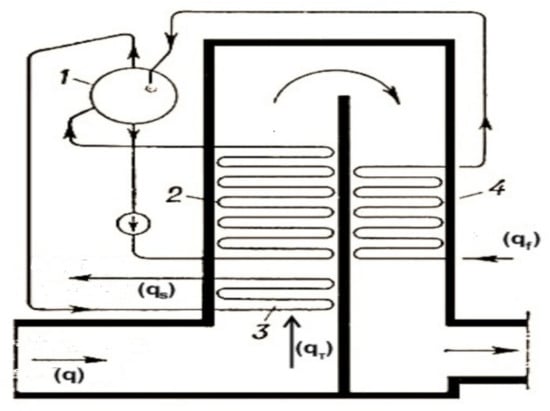
Figure 1.
Schematic of the utility boiler with forced circulation. Let us list the main parts of the boiler: 1—the drum; 2—the evaporation part; 3—the superheater; 4—the water economizer.
The control plant model consists of three interconnected circuits with input actions (controls) and output (controlled) variables , where:
- is feed water consumption ;
- is the heat flow in the pipe ;
- is the flow rate thermostat ;
- is the water level in the drum ;
- is the drum pressure ;
- is the steam temperature [°C].
The goal of the control is to keep the output variables at a given level. To describe the controlled processes, we can use the mathematical models proposed in [2].
The steam flow rate is a function of the steam pressure difference between the drum and the header. Using a modified form of Bernoulli’s law, we obtained the following relationship
where is a constant and and is the steam pressure in the drum and in the last stage of the superheater header, respectively.
To study the dynamics of pressure in the drum, the following empirical model was adopted
where the constant parameters were determined from the data on the steady load modes of the waste heat boiler.
Determining the water level in the drum is a difficult problem. Indirectly, the water level in the drum was determined based on the following considerations. Let be the total volume of the steam–water mixture and be the fluid density, which are related by the following differential equation:
To study the water level in the system, we could write the following relationship
The steam temperature dynamics are described by a system of third-order differential equations. The empirical model for studying the steam temperature has the form:
where is steam temperature [°C], is outlet temperature [°C], and is steam mass content (%).
A distinctive feature of the mathematical model of the considered control plant is that all parameters in Equations (41)–(45) are positive. In [2], this linearized model was used for the Syncrude Canada Ltd. (SCL) waste heat boiler under the assumption that there are three main steady state modes of its operation at low, medium, and high loads, respectively.
With regard to system (41)–(45), the problem of regulation is posed, namely, with the help of feedback, and it is necessary to maintain the values of output variables at given levels . This problem is reduced to the problem of stabilization of tracking errors:
It was assumed that the output variables are measured and the current values of the function are known.
In the process of regulation, the following restrictions are imposed on control actions:
4.2. Basic Control Laws
Let us use the ideology of the block approach [13,22] and divide the problem of synthesizing the tracking system into three independently solvable subproblems of a lower dimension.
At the first stage, the problem of maintaining the pressure in the drum at a given level is considered, which is the main one, while the other two subproblems (regulating the water level in the drum and the steam temperature) are considered auxiliary. The problem is that when solving control problem (46), it is necessary to ensure the fulfillment of conditions (47), i.e., the control action can take only non-negative values.
Let us present Equation (42), which describes the pressure dynamics in the drum with respect to the tracking error . Taking into account , we have:
where . Due to the , the free motion of system (48) is asymptotically stable; therefore, as shown in Section 2.1, the component can in principle be compensated using a non-negative control.
We chose the control in the form of a piecewise linear function of the second type (2)
We chose the parameters based on inequalities that are similar to those obtained in the analysis of system (8) and (9), namely:
where
and (47).
After entering the linear zone , the control is equal , and after substitution into (48), it can be seen that in a closed system
control goal (46) is achieved.
The results presented are practically significant if relation (47) is fulfilled. Note that one can influence the choice of amplitude by changing the gain . In addition, the amplitude also depends on the constraints on the control and its derivative , determined at the second stage.
The derivative of control is given by
and the following estimate holds Taking into account (50) and (51), we can write:
Next, we have the estimate
It can be seen from relation (52) that the upper (sufficient) estimate for the control derivative can be reduced by reducing the gain , and in addition, by limiting the control derivative . Thus, the constraint on the control derivative (47) is satisfied if
Note that as a result of stabilization of the tracking error (taking into account ), the mathematical model of the control plant (41)–(45) can be represented in a linear form, taking into account
Note that to eliminate the static tracking error, control (49) should be supplemented with an integral link
At the second stage, we can write a model that describes changes in the water level in the drum (43) and (44) under the following assumptions. According to the results of the first stage in the steady state, the steam consumption is a constant value and control operates in the linear zone
We can form the feedwater flow control as the output of a dynamic compensator of the form
For system (54), the following facts are obvious [21]. Let . Then, the following relations are valid:
Under these assumptions, the dynamic model of tracking error , taking into account (43), (44), (46), (53) and (54), has the form:
We chose a new control in the form of a piecewise linear function of the second type (2):
Let us show that by choosing the amplitude , it is possible to ensure the convergence to zero of the variables of the closed systems (55) and (56), taking into account and checking the convergence condition . If then , and taking into account (54) and , we have . If then , or taking into account , we have The choice of amplitude guarantees .
Equation (55) in the steady state implies equality . After substituting the equivalent control into (54), we have from which the steady-state values of the real control can be estimated as follows:
From Equation (48) in the steady state , we could obtain the steady value of the real control :
At the third stage, taking into account the results of the second stage, namely, we can write Equation (45) for the tracking error in the form
where the quantities
are considered as constant external disturbances. It is important that open-loop system (57) is stable for the parameters chosen below and the system matrix has eigenvalues
Let us consider some variants of the control action synthesis in system (57).
Variant 1. If the rate of convergence of open-loop system (57) is satisfactory, then we can choose the control as a function of constant disturbances. After equating the right-hand sides of (57) to zero, we have
From equating the right side of the last expression to zero, we have
To fulfill the control constraint (unipolarity requirement) for all three modes, the following implementation of the control action (58) is proposed:
Note that algorithms (58) and (59) do not use information about the state variables of system (57). In other words, control (58) is not a feedback control, and as a result, such a control algorithm is not rough to the variation of parameters.
Variant 2. In the general case, in the problem of tracking error stabilization as applied to system (57), we can follow the procedure from Section 3. Using a nondegenerate transformation of variables
we can transform it to a form similar to (33),
where
We note that the solutions of the equations of internal dynamics (the last two equations of system (60)) are unbounded, since the matrix of proper motions of the subsystem of zero dynamics at has the form
is not Hurwitz, and its eigenvalues are .
This means that it is impossible to directly use in the first subsystem (60) the combined control of the form Despite the fact that in this case, the first subsystem of system (60) is stable (the damping rate is determined by the choice of the gain ), the variables and consequently the control increase in absolute value without limit. In this case, one should use the recommendations on control synthesis in non-minimum phase systems (see Section 3).
In conclusion, we note that both considered variants of control synthesis have a common drawback, namely, they are not robust to the parametric uncertainties of system (60). To obtain robust steam temperature control algorithms in system (60), one should refer to the results of [7], where a solution to the tracking problem in non-minimal phase linear systems with one input and one output under conditions of parametric uncertainty and incomplete information about the state vector was proposed.
4.3. Simulation Results
Table 1 presents the steady-state values for the input and output variables of the waste heat boiler [2] for the three main modes.

Table 1.
Steady-state values for the input and output variables of the waste heat boiler.
Model parameters (2.1)–(2.5) were the same for all three modes: and
Only the corrections to the output variables were changed. involved taking values depending on one of the three steady-state modes (see Table 1).
The simulation was carried out in the MATLAB-Simulink environment. When modeling, the following parameters of control laws were adopted: in (48) and (49); in (55) and (56); in (57) and (59).
Figure 2, Figure 3 and Figure 4 show graphs of tracking errors for a given water level , pressure , and temperature during the transition of the control plant from one load mode to another, sequentially from low load to medium, then to high and back (see Table 1). Figure 5, Figure 6 and Figure 7 show the corresponding graphs of control actions and during the similar transition of the control plant from one load mode to another (see Table 1).
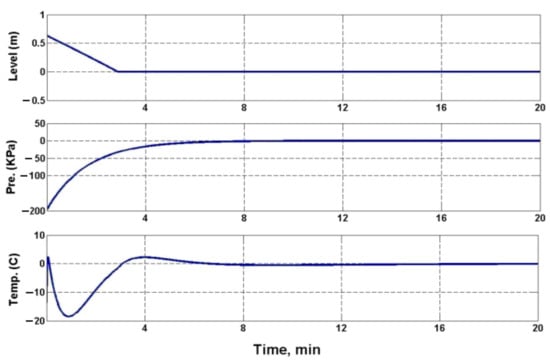
Figure 2.
Tracking error plots .
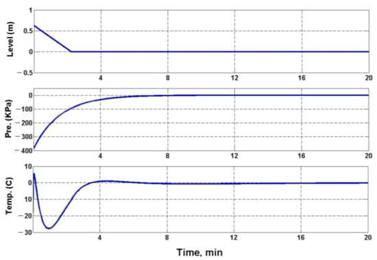
Figure 3.
Tracking error plots .
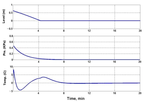
Figure 4.
Tracking error plots .
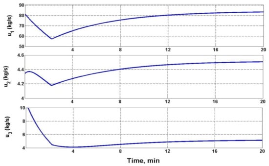
Figure 5.
Control action graphs .
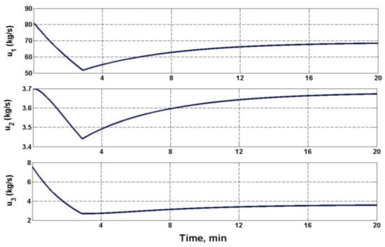
Figure 6.
Control action graphs .
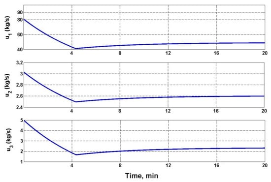
Figure 7.
Control action plots .
It can be seen from the figures that the processes in a closed system occurred sequentially according to the selected hierarchy of control loops: first, the steam pressure at the outlet of the waste heat boiler was set at a given level, then the set value of the water level was set, and finally, the set value of the superheated steam temperature was set.
5. Conclusions
In this paper, control algorithms for waste heat boilers were proposed, taking into account the restrictions on controls, which were formed in the form of linear functions with saturation using dynamic disturbance compensators. Taking into account the constraint on controls led initially linear models of control plants to nonlinear models. It is essential that the dynamic compensation method is not directly applicable to nonlinear systems, and its extension to the nonlinear case (taking into account constraints on controls) is the main theoretical result of this study.
In the theoretical part of the work, the main attention was paid to the problem of regulation by output variables under the action of constant disturbances and tasks (settings) using the method of dynamic disturbance compensation as applied to multiply connected linear systems. These results were applied to the synthesis of control laws for waste heat boilers. In particular, a step-by-step procedure was proposed that made it possible to linearize the model of the control plant by feedback due to the hierarchical sequence of solving control problems in separate circuits. To compensate for external disturbances and parametric uncertainties, the method of dynamic compensation was used, taking into account restrictions on controls.
When implementing the step-by-step procedure, in addition to the decomposition of the high-dimensional synthesis problem, it became possible at the first step to linearize the system after working out the given pressure in the drum. At the second step (water level), it became possible to assume that the disturbances in the remaining system are constant, and at the third step, it was possible to synthesize a controller of steam temperature without directly measuring it.
The effectiveness of the proposed algorithms was confirmed by numerical simulation in the MATLAB environment.
In the future, it is planned to apply the results obtained in the framework of this study to a number of applied problems of control to a nonlinear case, in particular, heat and power plants.
Author Contributions
Conceptualization and methodology, S.A.K. and V.A.U.; validation, investigation, and formal analysis, A.V.U. and S.A.K.; writing—original draft preparation, S.A.K. and V.A.U.; writing—review and editing, A.V.U. All authors have read and agreed to the published version of the manuscript.
Funding
This research received no external funding.
Conflicts of Interest
The authors declare no conflict of interest.
References
- Johan, A.K.; Bell, R.D. Drum boiler dynamics. Automatica 2000, 36, 363–378. [Google Scholar]
- Labibi, B.; Marquez, H.J.; Chen, T. Decentralized robust PI controller design for an industrial utility boiler. J. Process Control 2009, 19, 216–230. [Google Scholar] [CrossRef]
- Swarnakar, A.; Marquez, H.J.; Chen, T. Robust output feedback stabilization of nonlinear interconnected systems with application to an industrial utility boiler. In Proceedings of the IEEE Transactions on American Control Conference, Minneapolis, MN, USA, 14–16 June 2006; pp. 857–862. [Google Scholar]
- Ponce, I.U.; Bentsman, J.; Orlov, Y.; Aguilar, L.T. Aguilar generic nonsmooth output synthesis: Application to a coal-fired boiler/turbine unit with actuator dead zone. IEEE Trans. Control Syst. Technol. 2015, 23, 2117. [Google Scholar] [CrossRef]
- Wonham, W.F. Linear Multivariate Control: A Geometric Approach; Springer: New York, NY, USA, 1985. [Google Scholar]
- Singh, A.K.; Pal, B.C. An extended linear quadratic regulator for LTI systems with exogenous inputs. Automatica 2017, 76, 10–16. [Google Scholar] [CrossRef] [Green Version]
- Benevides, J.R.S.; Paiva, M.A.D.; Simplício, P.V.G.; Inoue, R.S.; Terra, M.H. Disturbance observer-based robust control of a quadrotor subject to parametric uncertainties and wind disturbance. IEEE Access 2022, 10, 7554–7565. [Google Scholar] [CrossRef]
- Rios, H.; Efimov, D.; Moreno, J.A.; Perruquetti, W.; Escobedo, J.G.R. Time-varying parameter identification algorithms: Finite and fixed-time convergence. IEEE Trans. Autom. Control 2017, 62, 3671–3678. [Google Scholar] [CrossRef] [Green Version]
- Afri, C.; Andrieu, V.; Bako, L.; Dufour, P. State and parameter estimation: A nonlinear Luenberger observer approach. IEEE Trans. Autom. Control 2017, 62, 973–980. [Google Scholar] [CrossRef] [Green Version]
- Yang, Z.; Zhang, D.; Sun, X.; Ye, X. Adaptive exponential sliding mode control for a bearingless induction motor based on a disturbance observer. IEEE Access 2018, 6, 35425–35434. [Google Scholar] [CrossRef]
- Utkin, V.I.; Guldner, J.; Shi, J. Sliding Mode Control in Electromechanical Systems; CRC Press: New York, NY, USA, 2009. [Google Scholar]
- Loukianov, A.G.; Domínguez, J.R.; Castillo-Toledo, B. Robust sliding mode regulation of nonlinear systems. Automatica 2018, 89, 241–246. [Google Scholar] [CrossRef]
- Kim, S.-K.; Ahn, C.K. Robust invariant manifold-based output voltage-tracking controller for DC/DC boost power conversion systems. IEEE Trans. Syst. Man Cybern. Syst. 2021, 51, 1582–1589. [Google Scholar] [CrossRef]
- Khalil, H.K.; Praly, L. High-gain observers in nonlinear feedback control. Int. J. Robust Nonlinear Control 2014, 24, 993–1015. [Google Scholar] [CrossRef]
- Andrievsky, B.; Furtat, I. Disturbance observers: Methods and applications. I. methods. Autom. Remote Control 2020, 81, 1563–1610. [Google Scholar] [CrossRef]
- Chen, W.H.; Yang, J.; Guo, L.; Li, S. Disturbance-observer-based control and related methods: An overview. IEEE Trans. Ind. Electron. 2016, 63, 1083–1095. [Google Scholar] [CrossRef] [Green Version]
- Ogata, K. Modern Control Engineering, 4th ed.; Prentice-Hall: Upper Saddle River, NJ, USA, 2001. [Google Scholar]
- Utkin, V.A.; Utkin, V.I. Design of invariant systems by the method of motion separation. Autom. Remote Control 1983, 44, 1559–1566. [Google Scholar]
- Pan, H.; Sun, W.; Gao, H.; Jing, X. Disturbance Observer-based adaptive tracking control with actuator saturation and its application. IEEE Trans. Autom. Sci. Eng. 2016, 13, 868–875. [Google Scholar] [CrossRef]
- Campos, E.; Monroy, J.; Abundis, H.; Chemori, A.; Creuze, V.; Torres, J. A nonlinear controller based on saturation functions with variable parameters to stabilize an AUV. Int. J. Nav. 2019, 11, 211–224. [Google Scholar] [CrossRef]
- Gulyukina, S.I.; Utkin, V.A. A block approach to CSTR control under uncertainty, state-space and control constraints. Control Sci. 2021, 5, 43–52. [Google Scholar]
- Krasnova, S.A.; Utkin, V.A.; Utkin, A.V. Block approach to analysis and design of the invariant nonlinear tracking systems. Autom. Remote Control 2017, 78, 2120–2140. [Google Scholar] [CrossRef]
- Antipov, A.S.; Krasnova, S.A.; Utkin, V.A. Methods of ensuring invariance with respect to external disturbances: Overview and new advances. Mathematics 2021, 9, 3140. [Google Scholar] [CrossRef]
Publisher’s Note: MDPI stays neutral with regard to jurisdictional claims in published maps and institutional affiliations. |
© 2022 by the authors. Licensee MDPI, Basel, Switzerland. This article is an open access article distributed under the terms and conditions of the Creative Commons Attribution (CC BY) license (https://creativecommons.org/licenses/by/4.0/).