Towards Explainable Machine Learning for Bank Churn Prediction Using Data Balancing and Ensemble-Based Methods

Abstract

The diversity of data collected on both social networks and digital interfaces is extremely increased, raising the problem of heterogeneous variables that are not often favourable to classification algorithms. Despite the significant improvement in machine learning (ML) and predictive analysis efficiency for classification in customer relationship management systems (CRM), their performance remains very limited by heterogeneous data processing, class imbalance, and feature scales. This impact turned out to be more important for simple ML methods which in addition often suffer from over-fitting. This paper proposes a succinct and detailed ML model building process including cross-validation of the combination of SMOTE to balance data and ensemble methods for modelling. From the conducted experiments, the random forest (RF) model yielded the best performance of 0.86 in terms of accuracy and f1-scoreusing balanced data. It confirms the literature summary about this topic which shows that RF was among the most effective algorithms for customer predictive classification issues. The constructed and optimized models were interpreted by Shapley values and feature importance analysis which shows that the “age” feature was the most significant while “HasCrCard” was the less one. This process has proven effective in bridging previously reported research gaps and the resulting model should be used for supporting bank customer loyalty decision-making.

1. Introduction

Customer relation management (CRM) tools are increasingly enriched with the use of Artificial Intelligence (AI) through machine learning (ML) algorithms for real-time predictions [1,2]. Using ML algorithms in CRM may be intended to help companies to predict scores on their opportunities, potential customers and purchases, customer reliability and loyalty [3,4], detect credit and insurance fraud [5,6], customer satisfaction [7,8], predict personalized recommendations for products and services [9,10], or the potential churn risk (loss of customers or subscribers) [11,12,13,14]. In this wide range of potential applications of ML in CRM decision support systems, the particular case of customer churn prediction is particularly interesting. Churn customer forecasting is an activity performed to predict whether a customer will leave the company. In addition, this was inspired by the fact that there are about 1.5 million bank churn customers annually, which is increasing each year [15]. Indeed, if it is difficult to win a customer, it is very easy on the other hand to lose him. The automatic predictions of customer churn would therefore be crucial to orientate the marketing operations of loyalty. Facing these major challenges and tough competition, involving ML algorithms would be better than simple tools now at the center of the digitalization of all companies.

The literature shows that several works have already been proposed to address the churn prediction problem [14,16]. However, not only are most of them focused on telecom customer churn (more recurrent and sensitive) but also the data, methods and experimental processes raise doubts about the results. For different ML algorithms applications as for bank churn prediction, the reliability of the built model closely depends on the data features involved [17,18]. Nowadays, the bank churn data is not only limited to information entered manually by the customers (sometimes not very reliable) but also includes other data from very operational activities such as interactions (active member status), tenure, estimated salary, etc., and also data collected from external sources (such as social networks) to enrich the banking information management system [6,19]. We speak of heterogeneous data. The main characteristic of heterogeneous data is that they are of several types (numerical, Boolean, scaled, nominal, …) and are merged from many different sources. To achieve the best performance of prediction algorithms, a transformation of these heterogeneous data is needed by appropriate preprocessing methods. Its optimization is one of the main challenges as currently no ML algorithm well processes non-digital data. Optimizing the transformation of this mosaic dataset for better prediction performance is the first goal we seek to achieve during preprocessing.

The binary classification constitutes a major part of the predictive classification problems [20], especially concerning the CRM applications such as bank churn prediction. However, this classification most often suffers from the problem of imbalance between the classes, which means that the majority class often tends to corrupt the decisions of the model in its favor, knowing that it is most often not the target of future correction. For example, in the case of bank churn, we want to predict which customers are likely to close their accounts and try to retain them. However, this class target (although important for bank customer loyalty) is in the minority (statistically) compared to the opposite. Some algorithms such as support vector machine (SVM), Naive Bayes (NB), k nearest neighbours (KNN), etc. are very affected by the class imbalance and unilaterally favor the majority class [18]. Methods such as decision trees (DT) and the derived ensemble methods are somewhat resistant to the impact of the majority class but the data balancing improves and stabilizes their performance. Moreover, transformed data presents a problem of different variable scales which affect many ML model performances. Standardization is an additional step in dealing with this problem but it has an adverse or favorable effect on the performance of certain algorithms that are said to be unstable to variable scales; knowing that a very large scale difference is more favourable for overfitting. Choosing ensemble methods overcomes this problem without the need to normalize the data [21]. The second contribution of this paper is to use the synthetic minority oversampling technique (SMOTE) method to balance the data while the third one is the building of stable and better performing models based on an ensemble approach.

To be useful and convincing to the targeted banking stakeholders, the ML models should be as transparent as possible by explaining how they proceeded to provide their decision. Thus, the fourth contribution of our study consists of explaining the constructed model using two variables, one based on the analysis of the Shapley values [22] of the model and the other on the importance of the features [23].

Following this work, Section 2 will investigate the literature on the application of machine learning techniques in bank churn prediction. Section 3 will depict the proposed methodology which constructs balanced data to train and explain our models. Then, Section 4 will analyze the performance results of the experiment, explain the results, and finally, Section 5 will conclude our work.

2. Related Work

Based on previous research, data mining models are currently very much needed to support or apply the effects of a CRM strategy [1] and this need does not date from today but it is growing with the central place that data has taken in recent years. The choice of a data mining model is based on the key CRM issues that the article wants to address. For example, clustering models are used more often for problems of automatic recommendation of products and services to customers [2,24], regression models are able to predict customer scoring, while classification models are more useful for predicting potential targets, reliability, loyalty and satisfaction [2] or customer churn prediction [11,12,13,14]. However, classification algorithms remain the most widely used for churn modeling and CRM learning problems. We can segment specific parts of a lead into groups to form an initial class of classification model strategy [1,25,26]. E.W.T. Ngai strategy [1] asserts for example that concerning loyalty programs, 83.3% used classification models to assist in decision-making. Furthermore, these problems often come down to the binary classification for which the most used methods are: SVM [27,28], DT [29,30,31], ANN [32,33], RF [30,31,34,35], etc. Among these works, only one [36] has addressed the problem of modeling bank churn in the form of clustering using the k-means algorithm, which has been outperformed by the KHM algorithm.

Overall, the task of automatic prediction of banking churn results, does not really have a classical dataset as for other problems, knowing that the subject is very active, the datasets often differ from one study to another depending on the country of the authors. which we present in more detail in Section 4.1. Various datasets have been used to test the majority of approaches proposed in the literature to predict the risk of bank churn. To better analyze the literature concerning the works publishing these approaches, we conducted a systematic survey to answer the questions:

• In which year was the paper published?
• Which ML algorithms were tested, which was the best and with what performance?
• What metrics were used to evaluate the proposed method(s)?
• Did the authors balance the data?
• Did the authors explain or interpret the ML models constructed?

The answers to the questions in this survey provide key information and even a benchmark on the elements involved in the process of building an efficient ML algorithm for the bank churn prediction task. The survey results are summarized in

Table 1. Summary of papers using ML for bank churn prediction. The best models are in bold.

Ref	Year	Algorithm	Metrics	Best Score	Balancing Data?	Explained Model?
[29]	2016	DT	Acc, pre, rec, f1	99.7, 91.8, 91.0, 90.96	No	Yes
[32]	2016	ANN	Acc	0.89	No	No
[37]	2014	SVM	Acc, sen, spe	83.1, 79.7, 83.7	No	No
[15]	2019	SVM	recall	0.73	Yes	No
[38]	2021	RF	Acc, AUC, f1	0.92, 0.91, 0.92	No	Yes
[35]	2020	RF	Acc, spe, sen, AUC	0.8, 0.81, 0.79, 0.84	No	Yes
[34]	2022	SVM, RF	Acc, f1	88.7, 91.90	Yes	No
[31]	2022	DT, KNN, SVM, RF	AUC	0.9	No	Yes
[36]	2019	k-means, KHM	Acc	91.4	No	No
[30]	2020	RF, DT	pre, f1	0.99, 0.76	Yes	No

below.

Table 1 summarizes the relevant papers that have dealt with direct bank churn prediction using machine learning approaches. It also gives details about the years of publication, the algorithms used, the performance metrics, the best scores and if the balancing of the data and the explanation (interpretation) of the model have been done. The topic has been active for a long time and is still active today with several publications in the year 2022. Among the most used ML algorithms, we have RF which most often gives the best performance, DT, SVM, etc. The most commonly used metrics include accuracy first, then specificity, sensitivity, precision, and recall which are often compromised by the f1 score, and finally, the AUC (area under the curve). Only three studies have balanced the data [15,30,34] and four others explained their models by the importance of features [29,31,35,38] but none used Shapley values or an approach involving both data balancing and model explanation.

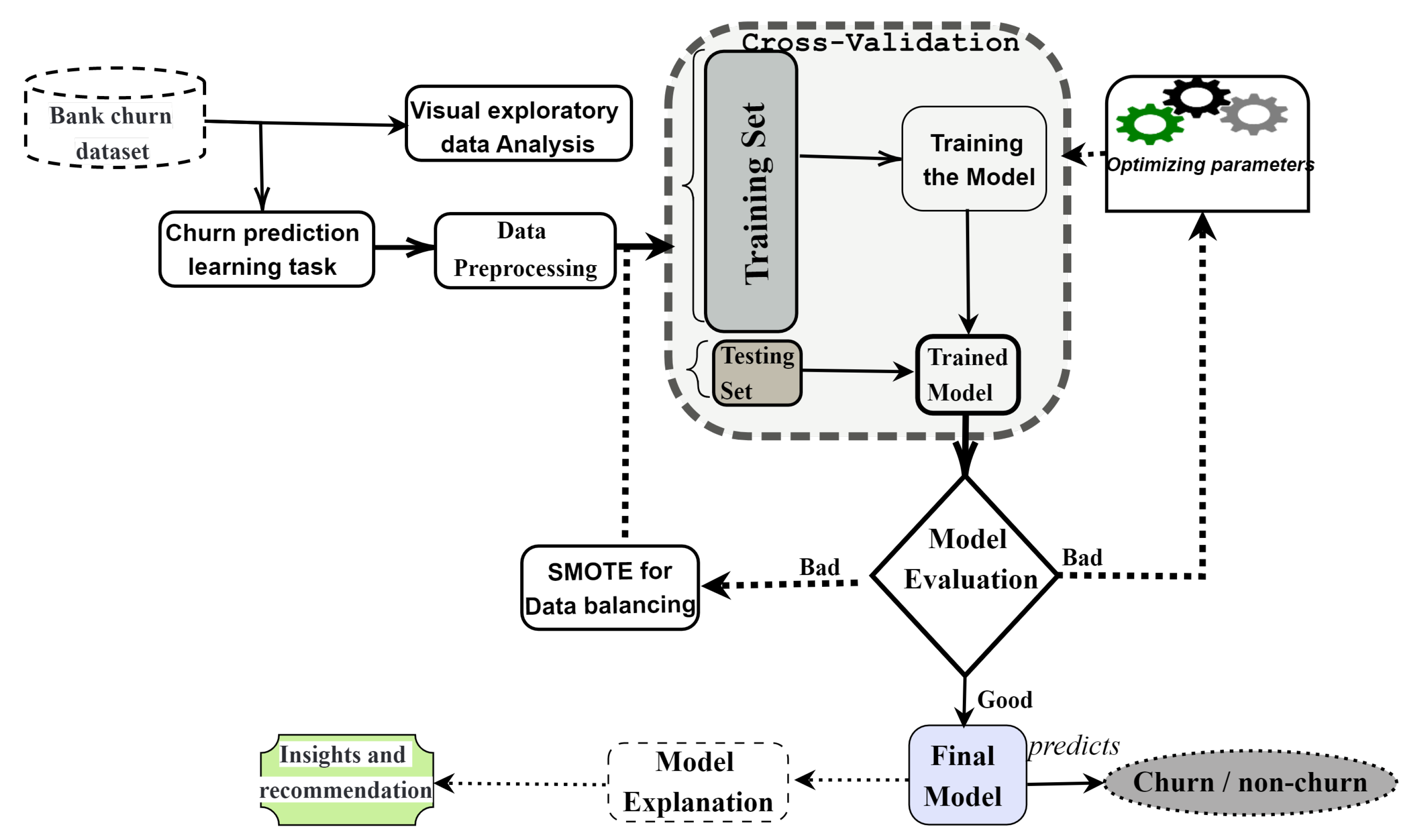
3. The Proposed Approach

Regarding the state of the art, we notice that ensemble methods have been little used for CRM prediction. However, this technique has proven itself in several challenges concerning predictive analysis. A concrete example remains its best performance at the Netflix challenge [39] which has made ensemble methods very famous and highly recommended for the scientific community. Several research contributions have been done to improve the ensemble methods which currently remain a major challenger of deep learning which is most used [21]. Recently, many studies [40,41,42,43] have shown that the combination of ensemble models with preprocessing techniques improves performance in modeling of the unbalanced classification problem. For a CRM dataset such as bank churn data having heterogeneous features and imbalance classes, appropriate data preprocessing is necessary to have the best model performance. Thus, the combination of features’ encoding, imbalanced processing techniques, and ensemble classifiers would improve the churn modeling prediction efficiency. Moreover, our model explanation by the joint analyses of Shapley values and features’ importance allow us to make reliable insights and recommendations to CRM managers on the indicators of variables directly affecting the bank churn decision. The flowchart in Figure 1 well depicts how we have constructed our proposed approach that will challenge existing approaches [30,31,34,36].

Following the collection of the bank customers’ churn data, we first perform their visual exploratory analysis to highlight the impact of the features on the customers’ churn decisions. After this analysis, the first step of our method is the data pre-processed (Section 3.1) before then starting the machine learning process to build the predictive model based on the ensemble methods (Section 3.3). The training data is first balanced by the SMOTE algorithm (Section 3.2) to mitigate the effects of the majority class on the algorithms’ efficiency. The constructed model is optimised and finally explained by the analysis of shap values and feature importance (Section 3.4).

3.1. Data Preprocessing

The preprocessing step turns out to be very important for the prediction process because the performance closely depends on it. Indeed, heterogeneous data are of different types including numerical, scaled, nominal, Boolean, etc. Since our dataset does not contain any missing values, the preprocessing of the data will consist much more of the transformation of the non-numerical data and the balancing. For the transformation of the non-numerical data, we followed the protocol used in [17,18] which consists of transforming specifically each categorical variable according to whether it is scaled, boolean or pure nominal.

3.2. SMOTE Method for Data Balancing

During the preprocessing phase, it is important to balance the instances of class records for accurate results. Refs. [30,34] used the imbalance methods including the synthetic minority oversampling technique (SMOTE) [44,45] algorithm, random oversampling (ROS), Random Balance (RB) [46], etc. in a similar context. In their work, the SMOTE algorithm proved to be the most relevant for balancing the data. Concerning random under-sampling of the majority class, previous authors have shown that this is not desirable, especially in combination with the ensemble method, as it can lead to data information loss [21]. SMOTE’s strategy is to create an artificial instance of a minority class through the following operating process: Considering an instance $x_i$ of the minority class, the algorithm starts by creating a new artificial instance from $x_i$ by first separating the k nearest neighbors to $x_i^{\prime }$, from the minority class. Then, randomly choose a neighbor and finally generate a synthetic example on the fictive line joining $x_i$ and the selected neighbor [21,40,44,47]. This process is clearly described by Algorithm 1. Several similar approaches will derive from this strategy, by which SMOTEBoost [48], Borderline-SMOTE [45], Majority-Weighted SMOTE [49], etc. However, we have not used them in this work for reasons of efficiency compared to SMOTE for VF data, but they could inspire many other researchers.

Algorithm 1 SMOTE algorithm [21]

Input: •      N: the number of instances in the minority classes;

•      n: the amount of SMOTE (in %);

•      $k$: the number of nearest neighbours;

•      minority data $D=x_i\in X,$ where $i=1,2,\dots ,N$.

Output: D′: synthetic data from D;

1: n ← (int)(n/100);

2: for i = 1 to N do

3:      Find the k nearest neighbours of $x_i$;

4:      while $n\ne 0$ do

5:            Select one of the k nearest neighbours of $x_i$

6:            Select a random number $\alpha \in$ [0, 1]

7:            x ← $x_i+\alpha (x-x_i)$

8:            Append x to D′

9:      end while

10: end for

3.3. Modelling and Prediction with Ensemble Methods

Ensemble-based methods consist of a combination of several independent basic classifiers that are in most cases decision trees (DT) but can also be artificial neural networks (ANN) or support vector machine (SVM), k-nearest neighbours (k-NN) or naive Bayes (NB) [21]. Each of these independent weak learners provides an alternative prediction of the whole problem and the final prediction results in a combination (usually by weighted or unweighted vote) of these alternative predictions [50]. The ensemble technique generally allows for more stable and accurate output prediction because the error is much smaller than that provided by one of the individual base models which form the ensemble model Ensemble learning techniques generally allow for more stable and accurate output predictions due to the much smaller errors than the individual basic models that make up the ensemble model [40,51]. The strategy involved in aggregation-weak learners is important and could affect the performance of the model [21]. Over time, several ensemble aggregation strategies have emerged, most of which are static or dynamic [40,52]. In each case, whether the final ensemble-based model corrects the error was actually done separately from the base model, significantly reducing the overall error. To be effective, the baseline model must be forced to meet two conditions: independence and being a weak learner with high diversity in terms of bias and variance [21]. This operation allows for building much more robust models allowing them to surpass the classical models not only in terms of performance but also by avoiding overfitting and by limiting data imbalance and the impact of variable scales.

3.4. Model Explanation with Shapley Values and Feature Importance

Explaining ML models remains one of its biggest challenges today. Indeed, an explained model gives more insights to support decision-making. However, when the ML model makes predictions, not all variables play the same role. Some variables have little effect, while others have a significant effect on model decision parameters. Calculating and analyzing the shape values allow us to know the contribution effect of each variable in prediction [53,54,55] that we also compare to the importance of the features [29,30,38]. Indeed, the objective of Shape and Shapely value as well as feature importance is to accurately quantify the contribution of each data feature in the final decision of the algorithm.

Shap values refer to Shapley values [56], a game theory jargon and these values are primarily composed of two elements: the game and the players, where “game” represents the outcome of the predictive model and “players” reflects the attributes of the model. Shapley calculates the value of each player’s input proportion to the game [53]. About our scenario, the SHAP value calculation is done by applying these components and determining the contribution proportion of each feature to the result of the model. The contribution sizes of individual players are processed by examining all possible combinations of i for all possible player coalitions or characteristics (i ranges from 0 to n), with n representing the total number of accessible features).

Unlike the importance of features which also plays the same role, the shap illustration highlights the positive and negative impact of each variable for the ML model. The visualization associated with the Shap values provides insight into the internal behavior of the predictive model used in this process and therefore, increases its transparency and reliability for users [54,55]. The shap strength visualization specifically provides an accessible overview of the variable indicators that influence the bank churn decision that non-technical users can quickly interpret.

4. Results Analysis and Discussion

This section discusses in turn the data used with exploratory visual analysis, the experimental protocol we followed and finally an in-depth analysis of the obtained results each time with the appropriate interpretation.

4.1. Bank Churn Dataset

The predictive modelling of customer churn consists of estimating the probability that a customer will be defected using historical, behavioural and socio-economic information. This prediction is very important because it can boost customer satisfaction and is likely to churn. It is generally approached by classification algorithms to learn the different models of churn and non-churn [57]. Nevertheless, the current overview classification algorithms are not well aligned with business objectives [58]. In our work, we handle bank churn data (https://www.kaggle.com/datasets/shrutimechlearn/churn-modelling of 10,000 customers in three countries including France, Germany and Spain.

Table 2. Details of bank churn dataset.

N	Attribute	Description	Type	Role
1	IDclient	A unique identifier for each customer	Categorical	feature
2	Surname	The surname of the customer	Categorical	feature
3	CreditScore	This number is between 300 and 850 and depicts the creditworthiness of a consumer	Numerical	feature
4	Gender	The customer’s gender: Female (0) and Male (1)	Boolean	feature
5	Age	The client’s current age, at the time of being a customer	Numerical	feature
6	Tenure	The number of years the client has been with the bank.	Numerical	feature
7	Balance	The actual bank balance of the customer	Numerical	feature
8	NumOfProducts	The number of banking products used by the client	Numerical	feature
9	HasCrCard	The number of credit cards obtained from the bank by the client	Boolean	feature
10	IsActiveMember	Binary status indicating whether or not the client was active with the bank before he left it.	Boolean	feature
11	EstimatedSalary	The estimated customers’ salary	Numerical	feature
12	Exited	Binary flag stating if the customer closed an account with the bank or not.	Boolean	target

gives more details about the data variables. The initial dataset contains 12 attributes including the target (Exited) which can take one of the values 0 (not exited) or 1 (exited) for each customer depending on whether the customer has quit or not. 2037 customers are tagged “exited” while 7963 are “not exited”, so it is an average imbalance between the two classes with a ratio of the majority class to the minority class. Since the “IDClient” and “Surname” variables were not significant in training the models, they were excluded before the machine learning steps. We will first try to do a visual exploratory analysis of our data in the next section.

4.2. Visual Exploratory Data Analysis

This section allows analyzing customer characteristics, such as geography, and age, balance, etc while highlighting how it affects customer decisions. Through these different analyses, the bank will be able to predict the savings behaviors of customers and identify which type of customer is most likely to make term deposits on the one hand or to predict future account closures to carry out the necessary loyalty actions [35]. The bank’s CRM can then focus its marketing efforts on these customers. This will not only allow the bank churn prevention but also increase customer satisfaction by reducing unwanted advertising to certain customers. To obtain a better understanding of the dataset, the distribution of key variables such as “age”, “geography”, “balance”, “estimated salary”, etc. and the relationships among them by graphical visualization of the following figures.

Figure 2a illustrates the age distribution of the clients: The bank clients in this dataset have a wide age range, from 18 to 92 years old with a standard deviation of 10.49 and a mean age of 39 years. However, the majority are between 30 and 40 years old (32 to 44 years old are in the 25th and 75th percentiles). The age distribution of the clients is fairly normal with moderate skewness and kurtosis values of 1.01 and 4.39, respectively. The Anderson-Darling statistic test is 142.19 which is well above each critical value for the corresponding significance level. For example, a significance level of $\alpha$ = 0.01 with a critical value of 1.092 shows that the results are significant at the 0.01 level of significance. The same analysis can be done for the other numerical variables. Correlating the age distribution with the target variable, as shown in Figure 2b, reveals that the age groups with the highest attrition rates are 45–55 and 55–65, while the rate is very low for those under 35.

The scatter matrix in Figure 3 reveals a very mixed relationship between age, balance, estimated salary, credit score, and target (Exited). To learn more, a correlation matrix was plotted with all quantitative variables in Figure 3. It is clear that the independent variables are not correlated at all with each other, which is quite good for the modeling. However, the strongest correlations are observed for the “age” and “balance” variables with the target. Their influence on the result of the campaign will be studied in more detail in the explanation of the models built in Section 4.5.

Figure 4 provides insights into the exploration of categorical variables and possibly indicators of variables that mostly affect the churn decision and that should be particularly targeted or controlled. As shown by bar charts in Figure 4a,c, female are more likely to churn than male members, and the same is true for non-active versus active members. Similarly, Figure 4b shows that German customers are two times churned more than French and Spanish customers. Finally, Figure 4d customers having a number of products of 3 or 4 should be closely screened because the churn rate is 100% and 82% for these two indicators, respectively.

4.3. Experimental Protocol

The purpose of this section is to highlight the different steps followed in the development of our simulation, the simulation tools, the experimental parameters related to both the data and models, then finally the performance evaluation metrics.

To detect the stability of the models on the different distributions of our dataset, we have evaluated them through the 5-fold cross-validation process as shown in Figure 5. All the experiments were carried out on a Windows operating system under python 3.7 involving principally Scikit-learn library [59]. We use the “Asus” brand computer having the following configuration: intel core i7 processor with 8 GB of RAM and an NVIDIA Geforce 930M for graphic card [21].

Regarding the models involved in our experiments, we first perform initial simulations of all models with default parameters to detect the most promising one for better performance. For the most promising model, we applied a grid search to determine its optimal parameters. After optimizing the model we explained its decision process through shape value analyses and the importance of the variables’ features.

Performance Measure

The predictive accuracy score of Equation (1) is the most commonly used classification metric, but it does not show how the model has correctly classified instances of minority classes, which are often the main purpose of this type of learning problem. Therefore, accuracy score is necessary but not sufficient as a performance metric for imbalanced classification problems. It is not an effective tool for evaluation. Knowing that our dataset is unbalanced [60], we will evaluate our models with additional performance measures and ideally f1-score. Indeed, f1-score is a compromise between precision and recall (also called TPR), thus taking into account both minority and majority classes [21]. The f1-score formula is given by Equation (2).

$$Accuracy-score=\frac{a+b}{b+c+d}$$

(1)

$$\mathrm{f}1\text{-}\mathrm{score}=\frac{2a}{2a+c+d}$$

(2)

a: represents the set of the correctly predicted “1”, b: is the set of the correctly predicted “0”, c: represents the number of false-positives, and d: refers to the number of false-negatives.

4.4. Results Analysis and Discussion

The main objective is to show the influence of hybrid imbalance and machine learning techniques in optimizing the performance of predictive analytic integrated into CRM which aims to conquer, acquire and retain target customers by predicting future churn. Cross-validation has been used to evaluate the involved models and the best one is interpreted through shap values and feature importance.

4.4.1. Cross-Validated Results without Balance Data

First, we evaluated the basic involved models without data balancing. The cross-validated results are illustrated in Figure 6 and the average scores are summered in

Table 3. Summary of the average cross-validated performance results of the models without and with data balancing. The best scores are highlighted in bold.

	ML Model		ML Model
Model	Accuracy	f1-Score	Accuracy	f1-Score
KNN	0.75	0.12	0.68	0.70
SVM	0.80	0.00	0.57	0.64
DT	0.79	0.50	0.80	0.80
LR	0.79	0.09	0.67	0.67
ANN	0.66	0.10	0.52	0.54
NB	0.79	0.13	0.72	0.74
RF	0.86	0.58	0.86	0.86
B	0.85	0.54	0.84	0.83
GB	0.87	0.59	0.84	0.84
ET	0.86	0.55	0.86	0.86
AB	0.86	0.57	0.83	0.83

. Without data balancing, the results were already quite interesting for the ensemble methods (RF, B, GB, ET, and AB) and simple machine learning-based methods (KNN, SVC, DT, LR, ANN, and NB). Among these ensemble-based methods, two stand out with the best performance notably RF and GB whose both average performance reached 0.86 and 0.66 for accuracy and f1-score, respectively. Moreover, the height of the boxes in Figure 6 show that the simple learning methods are more sensitive to the distribution of the data, thus unstable and especially very affected by the imbalance of the classes. Indeed, these methods predict the minority class only with an average score lower than 13% except for the decision trees.

For this first simulation, there is a large gap between the performance measured by accuracy and that of f1-score. This large gap in performance is due to the class imbalance data and this imbalance favors the majority class to the detriment of the minority class. To overcome this problem, it is necessary to balance the data for the two classes.

In the second experiment, we used the SMOTE method to balance the data between the two classes before using them to train the models. The SMOTE method has proved its effectiveness in several unbalanced class prediction problems. The cross-validated results, still in terms of accuracy and f1-score, are shown in Figure 7a,b, respectively. Once again the ensemble methods perform better overall than the individual methods. There is also near equality between the performances as measured by the accuracy and f1-score. This result shows that the minority class was predicted with the same chance as the majority class and more efficiently. RF and GB also keep the lead of the best performances.

These first two experiments allowed us to identify the most promising models in order to improve them by the optimization technique based on the grid search method before explaining them. In the following, we experiment only with the random forest method (RF) which is our best model.

4.4.2. Optimizing Random Forest Performances Results

Grid search is the most widely used parameter optimization technique in machine learning. However, many works lack transparency on this step. It consists of training the model with all the possible combinations of the different values that its key parameters can take to find the most efficient combination. This operation can be very time-consuming if the model is slow or if its parameters and their possible values are numerous. For the RF model in our case, its key parameters are the number of estimators which is 50, and the weak learner which is a decision tree with a random state.

4.5. Model Explanation

The ML models previously built often constitute black boxes which we interpret by analyzing the value of Shap and the importance of the features illustrated by Figure 8a,b, respectively.

The biggest difference between this shap value with the regular feature importance plots is that it shows the positive and negative relationships of the predictors with the target variable. Shap summary plot in Figure 8a looks dotty because it is made of all the dots in the train data. Both rankings aim to identify which feature or set of features influenced the prediction in descending order. The joint analysis of these two figures allows us to highlight two perspectives on the impacts of the “age” and “HasCrCard” variables, which for the first is by far the most important while the second is the least of all. The “Balance” characteristic is also among the most important variables according to both rankings. These two perspectives more or less validate the hypothesis put forward in Section 4.2 by doing the exploratory analysis of our data with the correlation matrices. It is also important to note that all the variables contribute to decision-making.

4.6. Discussion and Insights

Facing the diversification and the volume of data collected which are increasingly big and heterogeneous, the classification algorithms currently used are facing many challenges. Sometimes, they are limited by the size of the data which makes them slower and weakens their performance, the gap of scales between the variables that make them unstable, heterogeneity of data and especially non-numerical data that requires appropriate preprocessing affect the model performance. Moreover, when it comes to classification problems, more often than not there is an imbalance in the classes which greatly impacts the models. This impact turned out to be more important for simple ML methods such as SVM, KNN, DT, LR, etc., which in addition often suffer from overfitting. This paper proposed a succinct and detailed ML model-building process including cross-validation of the combination of SMOTE to balance data and ensemble methods for modelling. The constructed and optimized models were interpreted by analysis of shap value and feature importance. This process has proven to be effective in overcoming the problems previously reported by offering several insights for bank churn prediction issue.

Firstly, using data balancing methods like SMOTE would not only help improve the accuracy of the models but also make them more stable. The approach of [34] achieves best result when the SMOTE technique is applied to overcome the unbalanced dataset and also combines undersampling and oversampling. However, undersampling would not be highly recommended as it results in a loss of information that could have been used for the model.

Secondly, ensemble methods prove to be much more efficient than other methods, offering robust and stable models that are also resistant to the effects of feature scales and overfitting. The RF ensemble method has challenged other ML models in many studies which reinforce this hypothesis [30,31,34,35]. The robustness of these set methods makes it possible to avoid certain additional transformations during preprocessing such as the selection of attributes or the normalization of data.

Thirdly, the interpretation of the ML models built in parallel with the results of the exploratory data analysis gives perspectives on certain variables and indicators of variables that would directly or very little affect the bank churn decision. Thus, the age of bank customers would greatly affect their decision to churn, while the fact of having a credit card or not would have less impact. Indeed, [61] demonstrates that customer churn can be influenced by two other important factors: customer age and customer background. The investigation of [31] customers who have strong relationships with financial institutions, have a lot of goods and services, and borrow a lot from banks are less likely to close their accounts. A better understanding of churn features is expected to allow bank managers to consider several churn prevention strategies [29].

5. Conclusions and Perspectives

This paper discussed the explainable machine learning application to optimize the bank churn prediction by combining data balancing and ensemble based-methods. Its first summarizes the literature on this topic which shows that random forests and other ensemble methods were among the most promising algorithms for customer predictive classification issues. However, the classification problems, often suffer from data heterogeneity and class imbalance which greatly impact the machine learning models. This impact turned out to be more important for simple ML methods such as SVM, KNN, DT, LR, etc., which in addition often suffer from overfitting. This paper has proposed a succinct and detailed ML model building process including cross-validation of the combination of SMOTE to balance data and ensemble methods for modelling. RF model yielded the best performance of 0.86 in terms of accuracy and f1-score using balanced data. The constructed and optimized models were interpreted by analysis of shap value and feature importance analysis which show that the “age” feature was the most significant while “HasCrCard” was the less one. This process has proven to be effective in overcoming the previously reported research gaps and the obtained model should be used for customers that features are becoming more and more similar to the above-identified churn groups. Providing the facilities needed by clients, improving the service quality, identifying the needs of different groups, and improving customer service are included in these strategies [29].

References

1. Ngai, E.W.; Xiu, L.; Chau, D.C. Application of data mining techniques in customer relationship management: A literature review and classification. Expert Syst. Appl. 2009, 36, 2592–2602. [Google Scholar] [CrossRef]
2. Bahari, T.F.; Elayidom, M.S. An efficient CRM-data mining framework for the prediction of customer behaviour. Procedia Comput. Sci. 2015, 46, 725–731. [Google Scholar] [CrossRef] [Green Version]
3. Ranjan, J.; Bhatnagar, V. Critical success factors for implementing CRM using data mining. J. Knowl. Manag. Pract. 2008, 1, 7. [Google Scholar] [CrossRef]
4. Dick, A.S.; Basu, K. Customer loyalty: Toward an integrated conceptual framework. J. Acad. Mark. Sci. 1994, 22, 99–113. [Google Scholar] [CrossRef]
5. Chaudhary, K.; Yadav, J.; Mallick, B. A review of fraud detection techniques: Credit card. Int. J. Comput. Appl. 2012, 45, 39–44. [Google Scholar]
6. Bhattacharyya, S.; Jha, S.; Tharakunnel, K.; Westland, J.C. Data mining for credit card fraud: A comparative study. Decis. Support Syst. 2011, 50, 602–613. [Google Scholar] [CrossRef]
7. Garver, M.S. Using data mining for customer satisfaction research. Mark. Res. 2002, 14, 8. [Google Scholar]
8. Oralhan, B.; Kumru, U.; Oralhan, Z. Customer satisfaction using data mining approach. Int. J. Intell. Syst. Appl. Eng. 2016, 4, 63–66. [Google Scholar] [CrossRef] [Green Version]
9. Zhang, Z.; Lin, H.; Liu, K.; Wu, D.; Zhang, G.; Lu, J. A hybrid fuzzy-based personalized recommender system for telecom products/services. Inf. Sci. 2013, 235, 117–129. [Google Scholar] [CrossRef]
10. Díez, J.; Martínez-Rego, D.; Alonso-Betanzos, A.; Luaces, O.; Bahamonde, A. Optimizing novelty and diversity in recommendations. Prog. Artif. Intell. 2019, 8, 101–109. [Google Scholar] [CrossRef] [Green Version]
11. Au, W.H.; Chan, K.C.; Yao, X. A novel evolutionary data mining algorithm with applications to churn prediction. IEEE Trans. Evol. Comput. 2003, 7, 532–545. [Google Scholar]
12. Wei, C.P.; Chiu, I.T. Turning telecommunications call details to churn prediction: A data mining approach. Expert Syst. Appl. 2002, 23, 103–112. [Google Scholar] [CrossRef]
13. Verbeke, W.; Martens, D.; Baesens, B. Social network analysis for customer churn prediction. Appl. Soft Comput. 2014, 14, 431–446. [Google Scholar] [CrossRef]
14. Vafeiadis, T.; Diamantaras, K.I.; Sarigiannidis, G.; Chatzisavvas, K.C. A comparison of machine learning techniques for customer churn prediction. Simul. Model. Pract. Theory 2015, 55, 1–9. [Google Scholar] [CrossRef]
15. Karvana, K.G.M.; Yazid, S.; Syalim, A.; Mursanto, P. Customer churn analysis and prediction using data mining models in banking industry. In Proceedings of the 2019 International Workshop on Big Data and Information Security (IWBIS), Bali, Indonesia, 11 October 2019; pp. 33–38. [Google Scholar] [CrossRef]
16. Hung, S.Y.; Yen, D.C.; Wang, H.Y. Applying data mining to telecom churn management. Expert Syst. Appl. 2006, 31, 515–524. [Google Scholar] [CrossRef] [Green Version]
17. Tékouabou Koumétio, S.C.; Toulni, H. Improving KNN Model for Direct Marketing Prediction in Smart Cities. In Machine Intelligence and Data Analytics for Sustainable Future Smart Cities; Springer: Berlin/Heidelberg, Germany, 2021; pp. 107–118. [Google Scholar] [CrossRef]
18. Koumétio, C.S.T.; Cherif, W.; Hassan, S. Optimizing the prediction of telemarketing target calls by a classification technique. In Proceedings of the 2018 6th International Conference on Wireless Networks and Mobile Communications (WINCOM), Marrakesh, Morocco, 16–19 October 2018; pp. 1–6. [Google Scholar]
19. Cioca, M.; Ghete, A.I.; Cioca, L.I.; Gifu, D. Machine learning and creative methods used to classify customers in a CRM systems. In Applied Mechanics and Materials; Trans Tech Publications Ltd.: Bach, Switzerland, 2013; Volume 371, pp. 769–773. [Google Scholar]
20. Krawczyk, B. Learning from imbalanced data: Open challenges and future directions. Prog. Artif. Intell. 2016, 5, 221–232. [Google Scholar] [CrossRef] [Green Version]
21. Tékouabou, S.C.K.; Chabbar, I.; Toulni, H.; Cherif, W.; Silkan, H. Optimizing the early glaucoma detection from visual fields by combining preprocessing techniques and ensemble classifier with selection strategies. Expert Syst. Appl. 2022, 189, 115975. [Google Scholar] [CrossRef]
22. Konstantinov, A.V.; Utkin, L.V. Interpretable machine learning with an ensemble of gradient boosting machines. Knowl.-Based Syst. 2021, 222, 106993. [Google Scholar] [CrossRef]
23. Rodríguez-Pérez, R.; Bajorath, J. Interpretation of machine learning models using shapley values: Application to compound potency and multi-target activity predictions. J. Comput.-Aided Mol. Des. 2020, 34, 1013–1026. [Google Scholar] [CrossRef]
24. Alphy, A.; Prabakaran, S. A dynamic recommender system for improved web usage mining and CRM using swarm intelligence. Sci. World J. 2015, 2015, 193631. [Google Scholar] [CrossRef] [Green Version]
25. Chen, Y.L.; Hsu, C.L.; Chou, S.C. Constructing a multi-valued and multi-labeled decision tree. Expert Syst. Appl. 2003, 25, 199–209. [Google Scholar] [CrossRef]
26. Elmandili, H.; Toulni, H.; Nsiri, B. Optimizing road traffic of emergency vehicles. In Proceedings of the 2013 International Conference on Advanced Logistics and Transport, Sousse, Tunisia, 29–31 May 2013; pp. 59–62. [Google Scholar]
27. Lai, K.K.; Yu, L.; Wang, S.; Huang, W. An intelligent CRM system for identifying high-risk customers: An ensemble data mining approach. In International Conference on Computational Science; Springer: Berlin/Heidelberg, Germany, 2007; pp. 486–489. [Google Scholar]
28. Farquad, M.; Ravi, V.; Raju, S.B. Analytical CRM in banking and finance using SVM: A modified active learning-based rule extraction approach. Int. J. Electron. Cust. Relatsh. Manag. 2012, 6, 48–73. [Google Scholar] [CrossRef]
29. Keramati, A.; Ghaneei, H.; Mirmohammadi, S.M. Developing a prediction model for customer churn from electronic banking services using data mining. Financ. Innov. 2016, 2, 1–13. [Google Scholar] [CrossRef] [Green Version]
30. Li, B.; Xie, J. Study on the Prediction of Imbalanced Bank Customer Churn Based on Generative Adversarial Network. In Journal of Physics: Conference Series; IOP Publishing: Bristol, UK, 2020; p. 032054. [Google Scholar] [CrossRef]
31. de Lima Lemos, R.A.; Silva, T.C.; Tabak, B.M. Propension to customer churn in a financial institution: A machine learning approach. Neural Comput. Appl. 2022, 1–18. [Google Scholar] [CrossRef] [PubMed]
32. Bilal Zorić, A. Predicting customer churn in banking industry using neural networks. Interdiscip. Descr. Complex Syst. 2016, 14, 116–124. [Google Scholar] [CrossRef]
33. Boudhane, M.; Nsiri, B.; Toulni, H. Optical fish classification using statistics of parts. Int. J. Math. Comput. Simul. 2016, 10, 18–22. [Google Scholar]
34. Muneer, A.; Ali, R.F.; Alghamdi, A.; Taib, S.M.; Almaghthawi, A.; Ghaleb, E.A.A. Predicting customers churning in banking industry: A machine learning approach. Indones. J. Electr. Eng. Comput. Sci. 2022, 26, 539–549. [Google Scholar] [CrossRef]
35. Verma, P. Churn Prediction for Savings Bank Customers: A Machine Learning Approach. J. Stat. Appl. Probab. 2020, 9, 535–547. [Google Scholar] [CrossRef]
36. Naveen Sundar, G.; Narmadha, D.; Jebapriya, S.; Malathy, M. Optimized Methodology for Hassle-Free Clustering of Customer Issues in Banking. In Cognitive Informatics and Soft Computing; Springer: Berlin/Heidelberg, Germany, 2019; Volume 768, pp. 421–428. [Google Scholar] [CrossRef]
37. Farquad, M.A.H.; Ravi, V.; Raju, S.B. Churn prediction using comprehensible support vector machine: An analytical CRM application. Appl. Soft Comput. 2014, 19, 31–40. [Google Scholar] [CrossRef]
38. Deng, Y.; Li, D.; Yang, L.; Tang, J.; Zhao, J. Analysis and prediction of bank user churn based on ensemble learning algorithm. In Proceedings of the 2021 IEEE International Conference on Power Electronics, Computer Applications (ICPECA), Shenyang, China, 22–24 January 2021; pp. 288–291. [Google Scholar] [CrossRef]
39. Feuerverger, A.; He, Y.; Khatri, S. Statistical significance of the Netflix challenge. Stat. Sci. 2012, 27, 202–231. [Google Scholar] [CrossRef]
40. Roy, A.; Cruz, R.M.; Sabourin, R.; Cavalcanti, G.D. A study on combining dynamic selection and data preprocessing for imbalance learning. Neurocomputing 2018, 286, 179–192. [Google Scholar] [CrossRef]
41. Xiao, J.; Xie, L.; He, C.; Jiang, X. Dynamic classifier ensemble model for customer classification with imbalanced class distribution. Expert Syst. Appl. 2012, 39, 3668–3675. [Google Scholar] [CrossRef]
42. Woloszynski, T.; Kurzynski, M. A probabilistic model of classifier competence for dynamic ensemble selection. Pattern Recognit. 2011, 44, 2656–2668. [Google Scholar] [CrossRef]
43. Alhamidi, M.R.; Jatmiko, W. Optimal Feature Aggregation and Combination for Two-Dimensional Ensemble Feature Selection. Information 2020, 11, 38. [Google Scholar] [CrossRef] [Green Version]
44. Chawla, N.V.; Bowyer, K.W.; Hall, L.O.; Kegelmeyer, W.P. SMOTE: Synthetic minority over-sampling technique. J. Artif. Intell. Res. 2002, 16, 321–357. [Google Scholar] [CrossRef]
45. Han, H.; Wang, W.Y.; Mao, B.H. Borderline-SMOTE: A new over-sampling method in imbalanced data sets learning. In International Conference on Intelligent Computing; Springer: Berlin/Heidelberg, Germany, 2005; pp. 878–887. [Google Scholar] [CrossRef]
46. Díez-Pastor, J.F.; Rodríguez, J.J.; García-Osorio, C.; Kuncheva, L.I. Random balance: Ensembles of variable priors classifiers for imbalanced data. Knowl.-Based Syst. 2015, 85, 96–111. [Google Scholar] [CrossRef]
47. Faris, H.; Abukhurma, R.; Almanaseer, W.; Saadeh, M.; Mora, A.M.; Castillo, P.A.; Aljarah, I. Improving financial bankruptcy prediction in a highly imbalanced class distribution using oversampling and ensemble learning: A case from the Spanish market. Prog. Artif. Intell. 2020, 9, 31–53. [Google Scholar] [CrossRef]
48. Wu, Y.; Ding, Y.; Feng, J. SMOTE-Boost-based sparse Bayesian model for flood prediction. EURASIP J. Wirel. Commun. Netw. 2020, 2020, 1–12. [Google Scholar] [CrossRef] [Green Version]
49. Barua, S.; Islam, M.M.; Yao, X.; Murase, K. MWMOTE—Majority Weighted Minority Oversampling Technique for Imbalanced Data Set Learning. IEEE Trans. Knowl. Data Eng. 2014, 26, 405–425. [Google Scholar] [CrossRef]
50. Bolón-Canedo, V.; Alonso-Betanzos, A. Ensembles for feature selection: A review and future trends. Inf. Fusion 2019, 52, 1–12. [Google Scholar] [CrossRef]
51. Diez-Olivan, A.; Del Ser, J.; Galar, D.; Sierra, B. Data fusion and machine learning for industrial prognosis: Trends and perspectives towards Industry 4.0. Inf. Fusion 2019, 50, 92–111. [Google Scholar] [CrossRef]
52. Kuncheva, L.I. A theoretical study on six classifier fusion strategies. IEEE Trans. Pattern Anal. Mach. Intell. 2002, 24, 281–286. [Google Scholar] [CrossRef] [Green Version]
53. Padarian, J.; McBratney, A.B.; Minasny, B. Game theory interpretation of digital soil mapping convolutional neural networks. Soil 2020, 6, 389–397. [Google Scholar] [CrossRef]
54. Arjunan, P.; Poolla, K.; Miller, C. EnergyStar++: Towards more accurate and explanatory building energy benchmarking. Appl. Energy 2020, 276, 115413. [Google Scholar] [CrossRef]
55. Parsa, A.B.; Movahedi, A.; Taghipour, H.; Derrible, S.; Mohammadian, A.K. Toward safer highways, application of XGBoost and SHAP for real-time accident detection and feature analysis. Accid. Anal. Prev. 2020, 136, 105405. [Google Scholar] [CrossRef]
56. Lundberg, S.M.; Lee, S.I. A Unified Approach to Interpreting Model Predictions. In Proceedings of the 31st International Conference on Neural Information Processing Systems, NIPS’17, Long Beach, CA, USA, 4–9 December 2017; Curran Associates Inc.: Red Hook, NY, USA, 2017; pp. 4768–4777. [Google Scholar]
57. Bahnsen, A.C.; Aouada, D.; Ottersten, B. Example-dependent cost-sensitive decision trees. Expert Syst. Appl. 2015, 42, 6609–6619. [Google Scholar] [CrossRef]
58. Verbraken, T.; Verbeke, W.; Baesens, B. A novel profit maximizing metric for measuring classification performance of customer churn prediction models. IEEE Trans. Knowl. Data Eng. 2012, 25, 961–973. [Google Scholar] [CrossRef]
59. Raschka, S.; Mirjalili, V. Python Machine Learning: Machine Learning and Deep Learning with Python. In Scikit-Learn, and TensorFlow; Packt Publishing: Birmingham, UK, 2017. [Google Scholar]
60. Marinakos, G.; Daskalaki, S. Imbalanced customer classification for bank direct marketing. J. Mark. Anal. 2017, 5, 14–30. [Google Scholar] [CrossRef]
61. Chayjan, M.R.; Bagheri, T.; Kianian, A.; Someh, N.G. Using data mining for prediction of retail banking customer’s churn behaviour. Int. J. Electron. Bank. 2020, 2, 303–320. [Google Scholar] [CrossRef]
Figure 1. Flowchart of the proposed approach.
Mathematics 10 02379 g001
Figure 2. Visualizing age variable (a) distribution and (b) group by exited status.
Mathematics 10 02379 g002
Figure 3. Correlation matrices between numerical variables and target variables.
Mathematics 10 02379 g003
Figure 4. Visualizing the churn rate by (a) Gender (b) Country, (c) Active member status, and (d) Number of products.
Mathematics 10 02379 g004
Figure 5. Illustration of the experimental protocol (a) without and (b) with data balancing.
Mathematics 10 02379 g005
Figure 6. Performance results without balanced data (a) accuracy score and (b) f1 score.
Mathematics 10 02379 g006
Figure 7. Performance results after using smote to balance the data (a) accuracy score and (b) f1-score.
Mathematics 10 02379 g007
Figure 8. Visualizing the model explanation with the plotting of (a) shap values and (b) features importance.
Mathematics 10 02379 g008