On Finite/Fixed-Time Stability Theorems of Discontinuous Differential Equations

Abstract

We investigated the finite/fixed-time stability (FNTS/FXTS) of discontinuous differential equations (DDEs) in this paper. To cope with differential equations that were discontinuous on the right-hand side, we utilized the Filippov solution, which is widely used in engineering. Under the framework of the Filippov solution, we transformed this issue into an FNTS/FXTS problem in the corresponding functional differential inclusion. We proposed some new FNTS/FXTS criteria, which will have important applications in the field of control engineering. It is worth mentioning that the coefficient function in the inequality satisfied by the Lyapunov function (LF) could be indefinite. Moreover, our paper gave a new estimation for the settling time (ST). Finally, two illustrative examples were given to demonstrate the validity and feasibility of the proposed criteria.

1. Introduction

The term finite-time stability (FNTS) has been used to refer to situations in which the trajectories of the system can converge to an equilibrium point in finite-time and remain there for the rest of the time. The rudiments of the definition of FNTS can be traced back to 1963. Compared to the traditional Lyapunov asymptotic stability and exponential stability, FNTS has fast convergence, high accuracy and good robustness against various uncertainties [1,2]. Moreover, it is more reasonable and easy to obtain in practical applications because of the limited time required. By virtue of its wide application in industrial engineering, the relevant research has attracted a large number of scholars, which contributed to its vigorous development in the 1990s. Especially, in the 2000s, Bhat et al. [3] analyzed the FNTS of continuous autonomous systems. Hong et al. [1] analyzed FNTS and designed feedback laws for the studied system by exploiting a novel definition of finite-time input-to-state stability. Furthermore, FNTS has also been extensively studied for multi-agent systems, hybrid systems and so on [4,5,6,7,8]. For instance, Chen et al. [9] deeply researched the FNTS problem in switched nonlinear systems by adopting the common indefinite Lyapunov function (LF) and multiple indefinite LFs. Based on coupled matrix inequalities, Xu et al. [10] proposed sufficient conditions to study the FNTS of linear singular impulsive systems.

In particular, it is worth pointing out that the estimation of settling-time (ST) depends on the initial values in FNTS; however, sometimes it is hard, or even impossible, to obtain in some practical systems, which makes it difficult to estimate the ST. To deal with this, Polyakov [11] first introduced the definition of FXTS and studied the FXTS of the linear systems through a nonlinear feedback control strategy. Moreover, in 2015, the author investigated the fixed-time convergence of multi-agent systems [12]. As defined, FXTS requires both Lyapunov stability and fixed-time convergence, and it generally requires a fixed upper bound on the FNTS-based ST. Due to the importance of FXTS, several significant research findings on it have been published. For instance, Ni et al. [13] presented a new system based on FXTS theory and a novel control scheme that can be implemented for the control and synchronization problems for many complex systems. In [14], the FXTS for higher-order systems was studied by exploiting the sign function and power integrator. Moreover, ref. [15] was the first to study FXTS with the existence of stochastic processes in systems and proposed a new concept of FXTS in probability. Hu et al. [16] investigated the FXTS of neural networks with delays and impulses. However, the above studies of FXTS were based on the traditional FXTS theorem with stringent conditions, where the coefficient of ${\mathcal{U}}^{\alpha }$ was restricted to be a negative constant. To this regard, we proposed new and more applicable FXTS criteria.

On the other hand, differential equations possessing discontinuity on the right-hand side have arisen in many fields, such as neural networks, economics, biology and control systems [17,18,19,20,21]. It is obvious that continuous differential equations cannot be used to describe the nature of discontinuous dynamical systems. Moreover, the previous methods of continuous differential equations cannot be directly applied to discontinuous differential equations. To solve the problem of discontinuity, the first important theoretical issue is to give a proper definition of the solutions of discontinuous systems [22]. Some definitions for solutions of differential equations possessing discontinuity on the right-hand side can be found in the literature [23,24]. In 1964, Filippov developed a new framework named the Filippov framework [23] and since then it has been extensively studied. In fact, by constructing appropriate set-valued mapping, we can study the solution of discontinuous differential equations by studying the solution of the corresponding differential inclusion. However, both FNTS and FXTS considered in the paper introduced above were obtained under a strict assumption, in which the dynamics of the differential equation were assumed to be continuous. Therefore, it is natural for us to ask the question as to whether the study of FNTS/FXTS can be generalized from continuous differential equations to discontinuous differential equations. Fortunately, there have been some outstanding studies in recent years. For example, Hu et al. [25] investigated FXTS of coupled neural networks that have discontinuous activation functions, and they designed a discontinuous control law to study fixed-time synchronization. In [26], the authors studied robust FNTS of fractional-order neural networks under the Filippov framework. Cai et al. [27] discussed the FNTS/FXTS of discontinuous systems where the LF had an indefinite derivative. Moreover, the proposed results were applied to neural networks possessing discontinuous activation. The shortcomings of the research discussed above inspired our interest in this field; hence, we gave some new criteria for the study of FNTS/FXTS for discontinuous differential equations, where the coefficients could be relaxed to be indefinite. Furthermore, our results gave a better estimate of the ST.

Based on the considerations above, we investigated the FNTS/FXTS of discontinuous differential equations under the framework of differential inclusion in this paper. Some new results for FNTS/FXTS have been acquired, and the coefficient function in the inequality satisfied by LF could be indefinite. The results were more general than those of the previous research and could be applied to many other systems. The structure of the following parts of this paper is as follows. We give the description of the discontinuous nonlinear systems and several preliminaries in Section 2. In Section 3, some FNTS/FXTS theorems of discontinuous differential equations and several corollaries are proposed. In Section 4, two illustrative examples are presented to verify the feasibility of our theorems.

Notations: let $\mathbb{R}$, ${\mathbb{R}}_{+}$, ${\mathbb{R}}_{-}$ be the set of real numbers, positive real numbers and negative numbers, respectively; ${\mathbb{R}}^n$ is an n-dimensional vector space and $2^{{\mathbb{R}}^n}$ is the family of all nonempty subsets of ${\mathbb{R}}^n$; given a set $\mathbb{A}\in {\mathbb{R}}_n$, $\mu \left(\mathbb{A}\right)$ is the Lebesgue measure of $\mathbb{A}$; $\overline{co}\left[\mathbb{E}\right]$ represents the closure of the convex hull of $\mathbb{E}$.

2. Materials and Methods

Let us propose a nonlinear discontinuous differential equation (DDE) whose model is of the following form:

$$\begin{array}{c}\hfill \left\{\begin{array}{cc}\hfill \dot{\eta }\left(t\right)& =g(t,\eta (t\left)\right),\hfill \\ \hfill \eta \left(t_0\right)& ={\eta }_0.\hfill \end{array}\right.\end{array}$$

(1)

where $\eta \left(t_0\right)={\eta }_0$ is the initial value, $\eta \left(t\right)\in {\mathbb{R}}^n$ is the state vector; $g:{\mathbb{R}}_{+}\times {\mathbb{R}}^n⟶2^{{\mathbb{R}}^n}$ is essentially locally bounded and Lebesgure measurable. Moreover, $g(t,\eta )$ is discontinuous on variable $\eta$.

Definition 1

([18]). For any $\eta \in \mathbb{Z}\subseteq {\mathbb{R}}^n$, if there is always a corresponding nonempty set $\mathcal{F}\left(\eta \right)\subseteq {\mathbb{R}}^n$, then we claim that $F:\eta ⟼\mathcal{F}\left(\eta \right)$ is a multi-valued map. Moreover, if there always exists a neighborhood $\mathcal{I}$ of ${\eta }_0$ such that $\mathcal{F}\left(\mathcal{I}\right)\subseteq \mathbb{N}$, where $\mathbb{N}$ is any open set containing $\mathcal{F}\left({\eta }_0\right)$, then F is upper semi-continuous (USC) at ${\eta }_0$.

Taking account of a Filippov set-valued map $\mathcal{G}(t,\eta ):{\mathbb{R}}_{+}\times {\mathbb{R}}^n⟶2^{{\mathbb{R}}^n}$, we have the following:

$$\mathcal{G}(t,\eta )=\underset{\sigma >0}{\cap }\underset{\mu \left(\mathbb{A}\right)=0}{\cap }\overline{co}\left[g(t,\mathbb{D}(\eta ,\sigma ))\right],$$

where $\mu \left(\mathbb{A}\right)$ indicates the Lebeague measure of $\mathbb{A}$ and $\mathbb{D}(\eta ,\delta )=\{y:\parallel \eta -y\parallel <\sigma \}$.

Definition 2

([27]). Given a non-degenerate interval $\mathbb{I}$, $\eta \left(t\right)$ is a function defined on it. $\eta \left(t\right)$ is called a Filippov solution of system (1) if it is absolutely continuous on any compact subset of $\mathbb{I}$. Moreover, it fulfils the following differential inclusion (DI):

$$\begin{array}{c}\hfill \left\{\begin{array}{cc}\hfill \dot{\eta }\left(t\right)& \in \mathcal{G}(t,\eta (t\left)\right),\hfill \\ \hfill \eta \left(t_0\right)& ={\eta }_0.\hfill \end{array}\right.\end{array}$$

(2)

Definition 3.

For system (2) and any $t\in {\mathbb{R}}_{+}$, we say ${\eta }^{*}$ is an equilibrium point of system if ${\eta }^{*}\in \mathcal{G}(t,{\eta }^{*})$. In addition, if $0\in \mathcal{G}(t,0)$, then we claim $\eta =0$ is a trivial solution of system (2).

Definition 4.

The trivial solution of system (1) [or system (2)] is

(i) 

FNTS, if it satisfies Lyapunov stability and finite-time attractiveness. Moreover, the finite-time attractiveness means that there exists a $T(t_0,{\eta }_0)>0$ satisfying $\underset{t⟶T(t_0,{\eta }_0)}{lim}\eta (t_0,{\eta }_0)\left(t\right)=0$ and $\eta (t_0,{\eta }_0)\left(t\right)=0$ for all $t\ge T(t_0,{\eta }_0)$, where $T(t_0,{\eta }_0)$ is known as the ST.

(ii) 

Uniformly FNTS, if it has uniform Lyapunov stability and finite-time attractiveness.

(iii) 

Uniformly FXTS, if it is uniformly FNTS and $T(t_0,{\eta }_0)$ is uniformly bounded with respect to ${\eta }_0$, i.e., there exists a fixed constant $T_{max}>0$ for any initial state point ${\eta }_0$ values satisfying $T(t_0,{\eta }_0)\le t_0+T_{max}$.

Lemma 1

([3]). For a Lyapunov function $\mathcal{U}(t,\eta (t\left)\right)$, if

(1) 

$\mathcal{U}(t,\eta (t\left)\right)$ is positive definite,

(2) 

$\mathcal{U}(t,\eta (t\left)\right)$ is radially unbounded and

(3) 

there exist $m>0$, $0<\alpha <1$, such that

$$\dot{\mathcal{U}}(t,\eta \left(t\right))\le -m{\mathcal{U}}^{\alpha }(t,\eta \left(t\right)),$$

(3)

then the origin of system (1) is said to be FNTS and the ST is estimated by

$$T(t_0,{\eta }_0)=t_0+\frac{1}{m(1-\alpha )}.$$

Lemma 2

([11]). For a Lyapunov function $\mathcal{U}(t,\eta (t\left)\right)$, if

(1) 

$\mathcal{U}(t,\eta (t\left)\right)$ is positive definite,

(2) 

$\mathcal{U}(t,\eta (t\left)\right)$ is radially unbounded and

(3) 

there exist $m,n>0$, $0<\alpha <1$ and $1<\beta$, such that

$$\dot{\mathcal{U}}(t,\eta \left(t\right))\le -m{\mathcal{U}}^{\alpha }\left(\eta \right)-n{\mathcal{U}}^{\beta }(t,\eta \left(t\right)),$$

(4)

then the origin of system (1) is said to be FXTS and the ST is estimated by

$$T(t_0,{\eta }_0)\le t_0+T_{max}=t_0+\frac{1}{m(1-\alpha )}+\frac{1}{n(\beta -1)}.$$

Definition 5.

If $\phi \in C[{\mathbb{R}}_{+}^1,{\mathbb{R}}_{+}^1]$ is monotonically strictly increasing in the domain of the definition and satisfies $\phi \left(0\right)=0$, then we say $\phi \in K$. If $\phi \in K$ and $\underset{s\to +\infty }{lim}\phi \left(s\right)=+\infty$, we denote $\phi \in K_{\infty }$.

Definition 6

([18]). The Clarke generalized gradient of a locally Lipschitz continuous (LLC) function $\mathcal{U}(t,\eta ):{\mathbb{R}}_{+}\times {\mathbb{R}}^n⟶\mathbb{R}$ at $(t,\eta )$ is defined by

$$\partial \mathcal{U}(t,\eta )=\overline{co}[\underset{k⟶+\infty }{lim}\nabla \mathcal{U}(t_k,{\eta }_k):(t_k,{\eta }_k)⟶(t,\eta ),(t_k,{\eta }_k)\notin S\cup \Omega ].$$

where S is a set satisfying $\mu \left(S\right)=0$ and for every point of Ω the derivative of $\mathcal{U}(t,\eta )$ does not exist.

Definition 7

([28]). Let $\mathcal{U}\left(\eta \right):{\mathbb{R}}^n⟶\mathbb{R}$ be an LLC function, $D^{+}\mathcal{U}(\eta ,w)$ denotes the right-upper Dini derivative and ${\overline{D}}_c\mathcal{U}(\eta ,w)$ denotes the generalized directional derivative of $\mathcal{U}$ at η. For any $w\in {\mathbb{R}}^n$, we say $\mathcal{U}\left(\eta \right)$ is regular at η if ${\overline{D}}_c\mathcal{U}(\eta ,w)=D^{+}\mathcal{U}(\eta ,w)$, where ${\overline{D}}_c\mathcal{U}(\eta ,w)$ is defined as follows:

$${\overline{D}}_c\mathcal{U}(\eta ,w)=\underset{h⟶0^{+}y⟶\eta }{lim\; sup}\frac{\mathcal{U}(y+hw)-\mathcal{U}\left(y\right)}{h}.$$

Definition 8

([28]). For function $\mathcal{U}\left(\eta \right):{\mathbb{R}}^n⟶\mathbb{R}$, if it is regular at every $\eta \in {\mathbb{R}}^n$, $\mathcal{U}\left(\eta \right)>0$ for any $\eta \ne 0$, $\mathcal{U}\left(0\right)=0$. Moreover, $\mathcal{U}\left(\eta \right)⟶+\infty$ when $\Vert \eta \Vert ⟶+\infty$. Then we say $\mathcal{U}\left(\eta \right)$ is C-regular.

Lemma 3

([28]). Assume that $\mathcal{U}(t,\eta ):{\mathbb{R}}_{+}\times {\mathbb{R}}^n⟶\mathbb{R}$ is C-regular, $\eta \left(t\right)$ is a function which is absolutely continuous. For $a.a.$$(t,\eta )\in {\mathbb{R}}_{+}\times {\mathbb{R}}^n$, we say $\mathcal{U}(t,\eta )$ is differentiable and

$$\dot{\mathcal{U}}(t,\eta )=<\vartheta (t,\eta ),{(1,{\left(\dot{\eta }\right)}^T)}^T>,$$

(5)

where $\forall \vartheta (t,\eta )\in \partial \mathcal{U}(t,\eta ).$

Lemma 4

([29]). If $\chi ={({\chi }_1,{\chi }_2,...,{\chi }_n)}^T$ with ${\chi }_s>0$ and $0<{\omega }_1<{\omega }_2$, then

$${\left(\sum _{s=1}^n{\chi }_s^{{\omega }_2}\right)}^{\frac{1}{{\omega }_2}}\le {\omega }_2{\left(\sum _{s=1}^n{\chi }_s^{{\omega }_1}\right)}^{\frac{1}{{\omega }_1}}\le {\omega }_2{n}^{\frac{1}{{\omega }_1}-\frac{1}{{\omega }_2}}{\left(\sum _{s=1}^n{\chi }_s^{{\omega }_2}\right)}^{\frac{1}{{\omega }_2}}.$$

Lemma 5

([30]). If ${\chi }_1,{\chi }_2,...,{\chi }_n\ge 0$, $0<{\omega }_1\le 1$, and ${\omega }_2>1$, then

$$\sum _{s=1}^n{\chi }_s^{{\omega }_1}\ge {\left(\sum _{s=1}^n{\chi }_s\right)}^{{\omega }_1},\sum _{s=1}^n{\chi }_s^{{\omega }_2}\ge n^{1-{\omega }_2}{\left(\sum _{s=1}^n{\chi }_s\right)}^{{\omega }_2}.$$

3. Results

By using the change in variables, we studied the stability of ${\eta }^{*}$ in DDEs (1) via the stability of $\eta =0$ to the corresponding DI (2) in this section. We also assumed that 0 was a trivial solution of system (1) or system (2). Sometimes we used $\mathcal{U}\left(t\right)$ to represent $\mathcal{U}(t,\eta (t\left)\right)$, and we used $\eta \left(t\right)$ to represent $\eta (t_0,{\eta }_0)\left(t\right)$$\eta (t,t_0,{\eta }_0)$.

Theorem 1.

Suppose the function $d_1\in K_{\infty }$, l(t) is an indefinite integral function, r(t) is a negative integral function. If there exists an LLC and C-regular function $\mathcal{U}:{\mathbb{R}}_{+}\times C([t_0,+\infty ),{\mathbb{R}}^n)⟶{\mathbb{R}}_{+}$, $\mathcal{U}(t,0)=0$ for all $t\in \mathbb{R}$, such that the following conditions hold:

(H₁):

$d_1(\parallel \eta \parallel )\le \mathcal{U}(t,\eta \left(t\right));$

(H₂):

$\dot{\mathcal{U}}(t,\eta \left(t\right))\le l\left(t\right){\mathcal{U}}^{\alpha }(t,\eta \left(t\right))+r\left(t\right){\mathcal{U}}^{\gamma +\mathrm{sign}(\mathcal{U}-1)}(t,\eta \left(t\right)),\mathrm{for}\mathrm{a}.\mathrm{e}.t\in [t_0,+\infty )$, where $0<\gamma -1\le \alpha <1$;

(H₃):

there exists ${\lambda }_1>0$ satisfying

$${\int }_{t^{{}^{\prime }}}^t[l^{+}\left(s\right)+r\left(s\right)]ds\le -{\lambda }_1(t-t^{{}^{\prime }}),\forall t^{{}^{\prime }},t\in [t_0,+\infty ),$$

where $l^{+}\left(s\right)=max\{l\left(s\right),0\}$, $l^{+}\left(s\right)+r\left(s\right)$ is a negative continuous function.

Then DI (2) is FNTS and the ST $T(t_0,{\eta }_0)$ can be calculated by

$$T(t_0,{\eta }_0)=t_0+\frac{{\mathcal{U}}^{1-\alpha }(t_0,\eta \left(t_0\right))}{(1-\alpha ){\lambda }_1}.$$

Proof. 

From $\left(H_2\right)$ and the negativity of $r\left(t\right)$, we have

$$\begin{array}{cc}\hfill \dot{\mathcal{U}}(t,\eta \left(t\right))& \le l^{+}\left(t\right){\mathcal{U}}^{\alpha }(t,\eta \left(t\right))+r\left(t\right){\mathcal{U}}^{\alpha }(t,\eta \left(t\right)),\hfill \\ \hfill & =[l^{+}\left(t\right)+r\left(t\right)]{\mathcal{U}}^{\alpha }(t,\eta \left(t\right)),\mathrm{for}\mathrm{a}.\mathrm{e}.t\in [t_0,+\infty ).\hfill \end{array}$$

(6)

Multiplying both sides of the above formula by ${\mathcal{U}}^{-\alpha }(t,\eta \left(t\right))$, then

$$\dot{\mathcal{U}}(t,\eta \left(t\right)){\mathcal{U}}^{-\alpha }(t,\eta \left(t\right))\le l^{+}\left(t\right)+r\left(t\right),\mathrm{for}\mathrm{a}.\mathrm{e}.t\in [t_0,+\infty ).$$

(7)

Which leads to

$${\dot{\mathcal{U}}}^{1-\alpha }(t,\eta \left(t\right))\le (1-\alpha )[l^{+}\left(t\right)+r\left(t\right)],\mathrm{for}\mathrm{a}.\mathrm{e}.t\in [t_0,+\infty ).$$

(8)

Integrating both sides of (8) from $t_0$ to t, one obtains

$${\mathcal{U}}^{1-\alpha }(t,\eta \left(t\right))\le {\mathcal{U}}^{1-\alpha }(t_0,\eta \left(t_0\right))+(1-\alpha ){\int }_{t_0}^t[l^{+}\left(s\right)+r\left(s\right)]ds,$$

(9)

because $l^{+}\left(s\right)+r\left(s\right)$ is negative, one gets

$${\mathcal{U}}^{1-\alpha }(t,\eta \left(t\right))\le {\mathcal{U}}^{1-\alpha }(t_0,\eta \left(t_0\right)).$$

(10)

Since $\mathcal{U}(t_0,0)=0$ and $\mathcal{U}(t,\eta (t\left)\right)$ is continuous, for $\forall ϵ>0$, $\forall t_0\ge 0$, there exists a $\sigma =\sigma (ϵ,t_0)$ such that for any $\parallel \eta \left(t_0\right)\parallel <\sigma$, one has that

$$\mathcal{U}(t_0,\eta \left(t_0\right))<d_1\left(ϵ\right).$$

(11)

Recalling the condition $\left(H_1\right)$, from (10) and (11), we deduced that

$$\begin{array}{cc}\hfill \parallel \eta \left(t\right)\parallel & \le d_1^{-1}\left(\mathcal{U}(t,\eta \left(t\right))\right)\le d_1^{-1}\left(\mathcal{U}(t_0,\eta \left(t_0\right))\right),\hfill \\ \hfill & <d_1^{-1}\left(d_1\left(ϵ\right)\right)=ϵ.\hfill \end{array}$$

(12)

We improved system (2) so that it realizes Lyapunov stability. Next we demonstrated the finite convergence of the trivial solution to system (2).

From the inequality (9), we derive that

$${\mathcal{U}}^{1-\alpha }(t,\eta \left(t\right))\le {\mathcal{U}}^{1-\alpha }(t_0,\eta \left(t_0\right))+(1-\alpha )[-{\lambda }_1(t-t_0)].$$

(13)

From (13), we have

$$\begin{array}{c}\hfill \mathcal{U}(t,\eta \left(t\right))\le {\{{\mathcal{U}}^{1-\alpha }(t_0,\eta \left(t_0\right))+(1-\alpha )[-{\lambda }_1(t-t_0)]\}}^{\frac{1}{1-\alpha }},\end{array}$$

(14)

make ${\mathcal{U}}^{1-\alpha }(t_0,\eta \left(t_0\right))+(1-\alpha )[-{\lambda }_1(t-t_0)]\le 0$, then $\mathcal{U}\left(t\right)$ is always equal to 0 when $t\ge T(t_0,\eta \left(t_0\right))$, where

$$T(t_0,\eta \left(t_0\right))=t_0+\frac{{\mathcal{U}}^{1-\alpha }(t_0,\eta \left(t_0\right))}{(1-\alpha ){\lambda }_1}.$$

(15)

Therefore, $\eta \left(t\right)$ is always equal to 0 when $t\ge T(t_0,\eta \left(t_0\right))$, the trivial solution of system (2) is finite-time convergence. Thus the trivial solution of system (2) is FNTS. The proof is completed. □

Theorem 2.

Suppose the function $d_1,d_2\in K_{\infty }$, l(t) is an indefinite integral function, r(t) is a negative integral function. If there exists an LLC and C-regular function $\mathcal{U}:{\mathbb{R}}_{+}\times C([t_0,+\infty ),{\mathbb{R}}^n)⟶{\mathbb{R}}_{+}$, $\mathcal{U}(t,0)=0$ for all $t\in \mathbb{R}$, such that the following conditions hold:

• $\left(H_1^{{}^{\prime }}\right):d_1(\parallel \eta \parallel )\le \mathcal{U}(t,\eta \left(t\right))\le d_2(\parallel \eta \parallel );$
• $\left(H_2\right):\dot{\mathcal{U}}(t,\eta \left(t\right))\le l\left(t\right){\mathcal{U}}^{\alpha }(t,\eta \left(t\right))+r\left(t\right){\mathcal{U}}^{\gamma +\mathrm{sign}(\mathcal{U}-1)}(t,\eta \left(t\right)),\mathrm{for}\mathrm{a}.\mathrm{e}.t\in [t_0,+\infty )$, where $0<\gamma -1\le \alpha <1$;
• $\left(H_3\right):$ there exists ${\lambda }_1>0$ such that

$${\int }_{t_0}^t[l^{+}\left(s\right)+r\left(s\right)]ds\le -{\lambda }_1(t-t_0),\forall t\in [t_0,+\infty ),$$

where $l^{+}\left(s\right)=max\{l\left(s\right),0\}$ and $l^{+}\left(s\right)+r\left(s\right)$ is a negative continuous function.

Then DI (2) is uniformly FNTS and the ST $T(t_0,{\eta }_0)$ can be calculated by

$$T(t_0,{\eta }_0)=t_0+\frac{{\mathcal{U}}^{1-\alpha }(t_0,\eta \left(t_0\right))}{(1-\alpha ){\lambda }_1}.$$

Proof. 

In Theorem 1, the finite-time convergence was been improved. Next, the uniform Lyapunov stability is improved. According to condition $\left(H_1^{{}^{\prime }}\right)$, we obtain

$$\mathcal{U}(t_0,\eta \left(t_0\right))\le d_2(\parallel \eta \left(t_0\right)\parallel ).$$

(16)

Recalling the inequality (10) and (16), one acquires

$$\mathcal{U}(t,\eta \left(t\right))\le \mathcal{U}(t_0,\eta \left(t_0\right))\le d_2(\parallel \eta \left(t_0\right)\parallel ).$$

(17)

Using the hypothesis $\left(H_1^{{}^{\prime }}\right)$, from (17) we derive

$$\parallel \eta \left(t\right)\parallel \le d_1^{-1}\left(\mathcal{U}(t,\eta \left(t\right))\right)\le d_1^{-1}(d_2(\parallel \eta \left(t_0\right)\parallel \left)\right).$$

(18)

For $\forall ϵ>0$, $\forall t_0\ge 0$, there exists a $\sigma =d_2^{-1}\left(d_1\left(ϵ\right)\right)$, such that for any $\parallel \eta \left(t_0\right)\parallel <\sigma$, it yields that

$$\begin{array}{cc}\hfill \parallel \eta \left(t\right)\parallel & \le d_1^{-1}(d_2(\parallel \eta \left(t_0\right)\parallel \left)\right),\hfill \\ \hfill & \le d_1^{-1}\left(d_2\right(d_2^{-1}\left(d_1\left(ϵ\right)\right)=ϵ.\hfill \end{array}$$

(19)

The $\sigma =d_2^{-1}\left(d_1\left(ϵ\right)\right)$ we selected was positive and independent on $t_0$, so we have improved the uniform Lyapunov stability. The proof is completed. □

Remark 1.

Compared to the conventional FNTS criterion $\dot{\mathcal{U}}(t,\eta \left(t\right))\le -m{\mathcal{U}}^{\alpha }(t,\eta \left(t\right))$ presented in Lemma 1 and the inequalities $\dot{\mathcal{U}}(t,\eta \left(t\right))\le l\left(t\right){\mathcal{U}}^{\alpha }(t,\eta \left(t\right))+r\left(t\right){\mathcal{U}}^{\gamma +\mathrm{sign}(\mathcal{U}-1)}$$(t,\eta \left(t\right))\le (l^{+}\left(t\right)+r\left(t\right)){\mathcal{U}}^{\alpha }(t,\eta \left(t\right))$, from this perspective, the more free variables, the more flexible the results.

Remark 2.

Because $l\left(t\right)+r\left(t\right)\le l^{+}\left(t\right)+r\left(t\right)$, if $l^{+}\left(t\right)+r\left(t\right)$ is negative, then $l\left(t\right)+r\left(t\right)$ is negative too, so the condition $\left(H_3\right)$ in Theorem 1 can be replaced by the condition ${\int }_{t_0}^{t}l\left(s\right)+r\left(s\right)ds\le -{\lambda }_1(t-t_0)$. Similarly, condition $\left(H_3\right)$ in Theorem 2 can be modified according to the same principle.

Theorem 3.

Let the condition in Theorem 2 hold, We can further demonstrate that DI (2) is uniformly FXTS and the ST $T(t_0,{\eta }_0)$ can be calculated as $T(t_0,{\eta }_0)\le t_0+T_{max}$, where

$$T_{max}=\frac{1}{\gamma {\lambda }_1}+\frac{1}{(1-\alpha ){\lambda }_1}.$$

Proof. 

DI (2) is shown to be uniformly FNTS by using the same method in Theorem 2. Next, we prove the ST is bounded. Firstly, we assert that there exists $t_0\le t^{*}\le T_1=t_0+\frac{1}{\gamma {\lambda }_1}$, such that $\mathcal{U}(t^{*},\eta \left(t^{*}\right))\le 1$. Otherwise, suppose $\mathcal{U}(t,\eta (t\left)\right)>1$ for all $t\in [t_0,T_1]$, from condition $\left(H_2\right)$ we get

$$\begin{array}{cc}\hfill \dot{\mathcal{U}}(t,\eta \left(t\right))& \le l\left(t\right){\mathcal{U}}^{\alpha }(t,\eta \left(t\right))+r\left(t\right){\mathcal{U}}^{\gamma +1}(t,\eta \left(t\right)),\hfill \\ \hfill & \le [l^{+}\left(t\right)+r\left(t\right)]{\mathcal{U}}^{\gamma +1}(t,\eta \left(t\right)),\mathrm{for}\mathrm{a}.\mathrm{e}.t\in [t_0,T_1].\hfill \end{array}$$

(20)

Multiplying both sides of (20) by ${\mathcal{U}}^{-\gamma -1}(t,\eta \left(t\right))$, one obtains

$$\dot{\mathcal{U}}(t,\eta \left(t\right)){\mathcal{U}}^{-\gamma -1}(t,\eta \left(t\right))\le l^{+}\left(t\right)+r\left(t\right),\mathrm{for}\mathrm{a}.\mathrm{e}.t\in [t_0,T_1].$$

(21)

That leads to

$$\frac{1}{-\gamma }{\dot{\mathcal{U}}}^{-\gamma }(t,\eta \left(t\right))\le l^{+}\left(t\right)+r\left(t\right),\mathrm{for}\mathrm{a}.\mathrm{e}.t\in [t_0,T_1].$$

(22)

Integrating both sides of (22) from $t_0$ to $T_1$, as $T_1=t_0+\frac{1}{\gamma {\lambda }_1}$, one acquires

$$\begin{array}{cc}\hfill \frac{1}{-\gamma }[{\mathcal{U}}^{-\gamma }(T_1,\eta \left(T_1\right))-{\mathcal{U}}^{-\gamma }(t_0,\eta \left(t_0\right))]& \le {\int }_{t_0}^{T_1}[l^{+}\left(s\right)+r\left(s\right)]ds,\hfill \\ \hfill & \le -{\lambda }_1(T_1-t_0)=\frac{1}{-\gamma }.\hfill \end{array}$$

(23)

Clearly, we can obtain ${\mathcal{U}}^{-\gamma }(T_1,\eta \left(T_1\right))\ge 1$, this contradicts $\mathcal{U}(T_1,\eta \left(T_1\right))>1$.

Secondly, from condition $\left(H_2\right)$, we obtain that

$$\begin{array}{cc}\hfill \dot{\mathcal{U}}(t,\eta \left(t\right))& \le l\left(t\right){\mathcal{U}}^{\alpha }(t,\eta \left(t\right))+r\left(t\right){\mathcal{U}}^{\gamma +\mathrm{sign}(\mathcal{U}-1)}(t,\eta \left(t\right)),\hfill \\ \hfill & \le l^{+}\left(t\right){\mathcal{U}}^{\alpha }(t,\eta \left(t\right))+r\left(t\right){\mathcal{U}}^{\alpha }(t,\eta \left(t\right)),\hfill \\ \hfill & =[l^{+}\left(t\right)+r\left(t\right)]{\mathcal{U}}^{\alpha }(t,\eta \left(t\right)),\mathrm{for}\mathrm{a}.\mathrm{e}.t\in [t^{*},+\infty ).\hfill \end{array}$$

(24)

Multiplying both sides of the above formula by ${\mathcal{U}}^{-\alpha }(t,\eta \left(t\right))$, one gets

$${\dot{\mathcal{U}}}^{1-\alpha }(t,\eta \left(t\right))\le (1-\alpha )[l^{+}\left(t\right)+r\left(t\right)],\mathrm{for}\mathrm{a}.\mathrm{e}.t\in [t^{*},+\infty ).$$

(25)

Integrating both sides of (25) from $t^{*}$ to t leads to

$$\begin{array}{cc}\hfill {\mathcal{U}}^{1-\alpha }(t,\eta \left(t\right))& \le {\mathcal{U}}^{1-\alpha }(t^{*},\eta \left(t^{*}\right))+(1-\alpha ){\int }_{t^{*}}^t[l^{+}\left(s\right)+r\left(s\right)]ds,\hfill \\ \hfill & \le 1+(1-\alpha )[-{\lambda }_1(t-t^{*})],\mathrm{for}\mathrm{a}.\mathrm{e}.t\in [t^{*},+\infty ).\hfill \end{array}$$

(26)

From the above equation, one gets

$$\begin{array}{c}\hfill \mathcal{U}(t,\eta \left(t\right))\le {\{1+(1-\alpha )[-{\lambda }_1(t-t^{*})]\}}^{\frac{1}{1-\alpha }}.\end{array}$$

(27)

In (27), we can make $1+(1-\alpha )[-{\lambda }_1(t-t^{*})]\le 0$, then $\mathcal{U}\left(t\right)$ is always equal to 0 when $t\ge t^{*}+\frac{1}{{\lambda }_1(1-\alpha )}$. As $t^{*}\le T_1=t_0+\frac{1}{\gamma {\lambda }_1}$, then

$$t\ge t_0+\frac{1}{\gamma {\lambda }_1}+\frac{1}{(1-\alpha ){\lambda }_1}\doteq t_0+T_{max}.$$

(28)

Therefore, $\eta \left(t\right)$ is always equal to 0 when $t\ge t_0+T_{max}$. Since the above expression for $T_{max}$ is independent of the initial value, we know that the trivial solution of system (2) is FXTS. The proof is completed. □

Remark 3.

In Theorems 1–3, the condition $\left(H_2\right)$ plays an important role in realizing FNTS/FXTS. In addition, $d_2(\parallel \eta \parallel )$ in Theorem 2 and Theorem 3 is used to realize the Lyapunov uniform stability.

Remark 4.

There exist some other criteria to guarantee FXTS, such as the conventional criterion $\dot{\mathcal{U}}\left(t\right)\le -a{\mathcal{U}}^{\alpha }\left(t\right)-b{\mathcal{U}}^{\beta }\left(t\right)$, where $0<\alpha <1$, $\beta >1$, see [11]; or $\dot{\mathcal{U}}\left(t\right)\le -a{\mathcal{U}}^{1-\frac{1}{2\theta }}\left(t\right)-b{\mathcal{U}}^{1+\frac{1}{2\theta }}\left(t\right)$, where $\theta >1$, see [31]; or $\dot{\mathcal{U}}\left(t\right)\le -a{\mathcal{U}}^{\frac{m}{n}}\left(t\right)-b{\mathcal{U}}^{\frac{p}{q}}\left(t\right)$, where $m>n$, $p<q$, and they are all positive odd integers, see [32]. We propose new FXTS criteria $\dot{\mathcal{U}}(t,\eta \left(t\right))\le l\left(t\right){\mathcal{U}}^{\alpha }(t,\eta \left(t\right))+r\left(t\right){\mathcal{U}}^{\gamma +\mathrm{sign}(\mathcal{U}-1)}(t,\eta \left(t\right))$ in this paper. It is worth stating that all existing results require that the coefficients in the inequalities satisfied by $\mathcal{U}\left(t\right)$ are negative. However, only $l^{+}\left(t\right)+r\left(t\right)$ needs to be negative in our results, and $l\left(t\right)$ can be indefinite. Thus the FXTS criteria proposed for the first time in this article were more general. Moreover, in Condition $\left(H_2\right)$, the coefficients $l\left(t\right)$ and $r\left(t\right)$ were allowed to be time-varying functions, while the results listed above all required the coefficients to be constants.

In Theorem 3, if $l\left(t\right)=l,r\left(t\right)=r$, then the following corollary can be drawn.

Corollary 1.

Suppose the function $d_1,d_2\in K_{\infty }$, $l\in \mathbb{R}$, $r\in {\mathbb{R}}_{-}$. If there is an LLC and C-regular function $\mathcal{U}:{\mathbb{R}}_{+}\times C([t_0,+\infty ),{\mathbb{R}}^n)⟶{\mathbb{R}}_{+}$, $\mathcal{U}(t,0)=0$ for all $t\in \mathbb{R}$, such that:

• $\left(H_1^{{}^{\prime }}\right):d_1(\parallel \eta \parallel )\le \mathcal{U}(t,\eta \left(t\right))\le d_2(\parallel \eta \parallel );$
• $\left(H_2^{{}^{\prime }}\right)$: $\dot{\mathcal{U}}(t,\eta \left(t\right))\le l{\mathcal{U}}^{\alpha }(t,\eta \left(t\right))+r{\mathcal{U}}^{\gamma +\mathrm{sign}(\mathcal{U}-1)}(t,\eta \left(t\right)),\mathrm{for}\mathrm{a}.\mathrm{e}.t\in [t_0,+\infty )$, where $l+r\le 0$, $0<\gamma -1\le \alpha <1$.

Then DI (2) is uniformly FXTS and the ST $T(t_0,{\eta }_0)$ can be calculated by

$$T(t_0,{\eta }_0)\le t_0+T_{max}=t_0+\frac{1}{-r\gamma }+\frac{1}{(1-\alpha )(-l-r)}.$$

Remark 5.

Li et al. investigated the fixed-time synchronization of complex dynamical networks by using FXTS criteria in [33]. If $l\in {\mathbb{R}}_{-}$, condition $\left(H_2^{{}^{\prime }}\right)$ in Corollary 1 will degenerate to the condition of the FXTS criteria in [33] when impulses are not present. Moreover, $T_{max}=\frac{1}{-r\gamma }+\frac{1}{(1-\alpha )(-l-r)}$ in Corollary 1 is smaller than $T_{max}=\frac{1}{-r\gamma }+\frac{1}{-l(1-\alpha )}$ in [33]. This means that the result in Corollary 1 is more relaxed and the estimation of ST is tighter.

Remark 6.

Theorems and corollaries in this paper could deal with discontinuous differential systems while the traditional theorems in [3,11,32] were only suitable for continuous differential systems. In this regard, our results were more applicable.

Remark 7.

Wang et al. [34] investigated the fixed-time convergence of systems and proposed a novel corresponding theorem. The derivative of $\mathcal{U}\left(t\right)$ satisfies $\dot{\mathcal{U}}\left(t\right)\le p_1\left(t\right){\mathcal{U}}^{\alpha }(t,\eta \left(t\right))+p_2\left(t\right){\mathcal{U}}^{\beta }(t,\eta \left(t\right))$, where $p_1\left(t\right)$ is an indefinite function, $p_2\left(t\right)$ is a non-positive function and $0<\alpha <1<\beta$. However, ref. [34] only proved fixed-time convergence without taking into account the Lyapunov stability problem. In this paper, we make clever use of $r\left(t\right){\mathcal{U}}^{\gamma +\mathrm{sign}(\mathcal{U}-1)}(t,\eta \left(t\right))$ to the equation and obtain the Lyapunov stability in Theorem 3, which implies we could obtain FXTS.

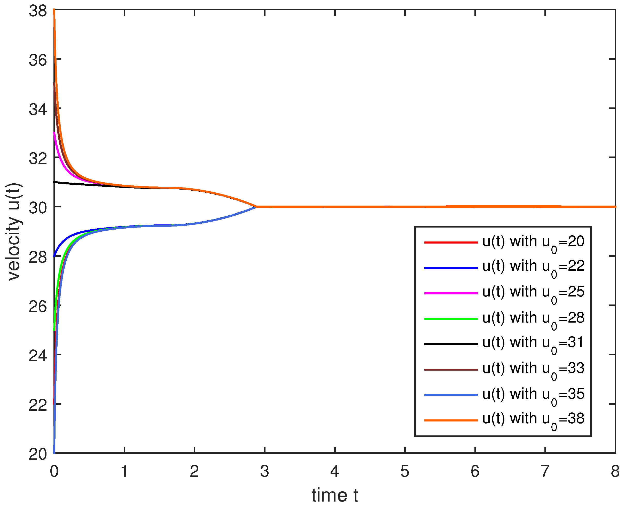
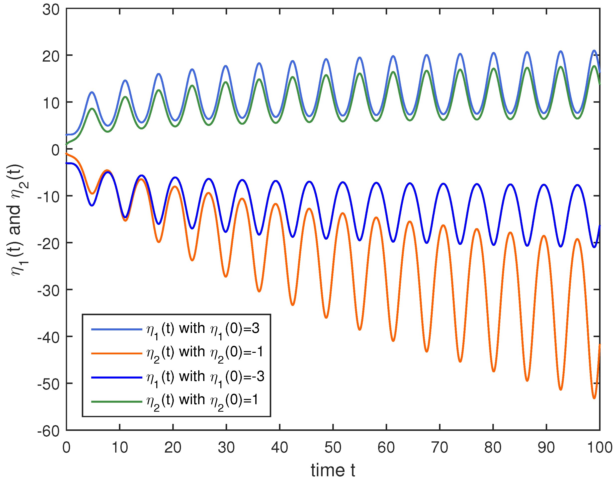
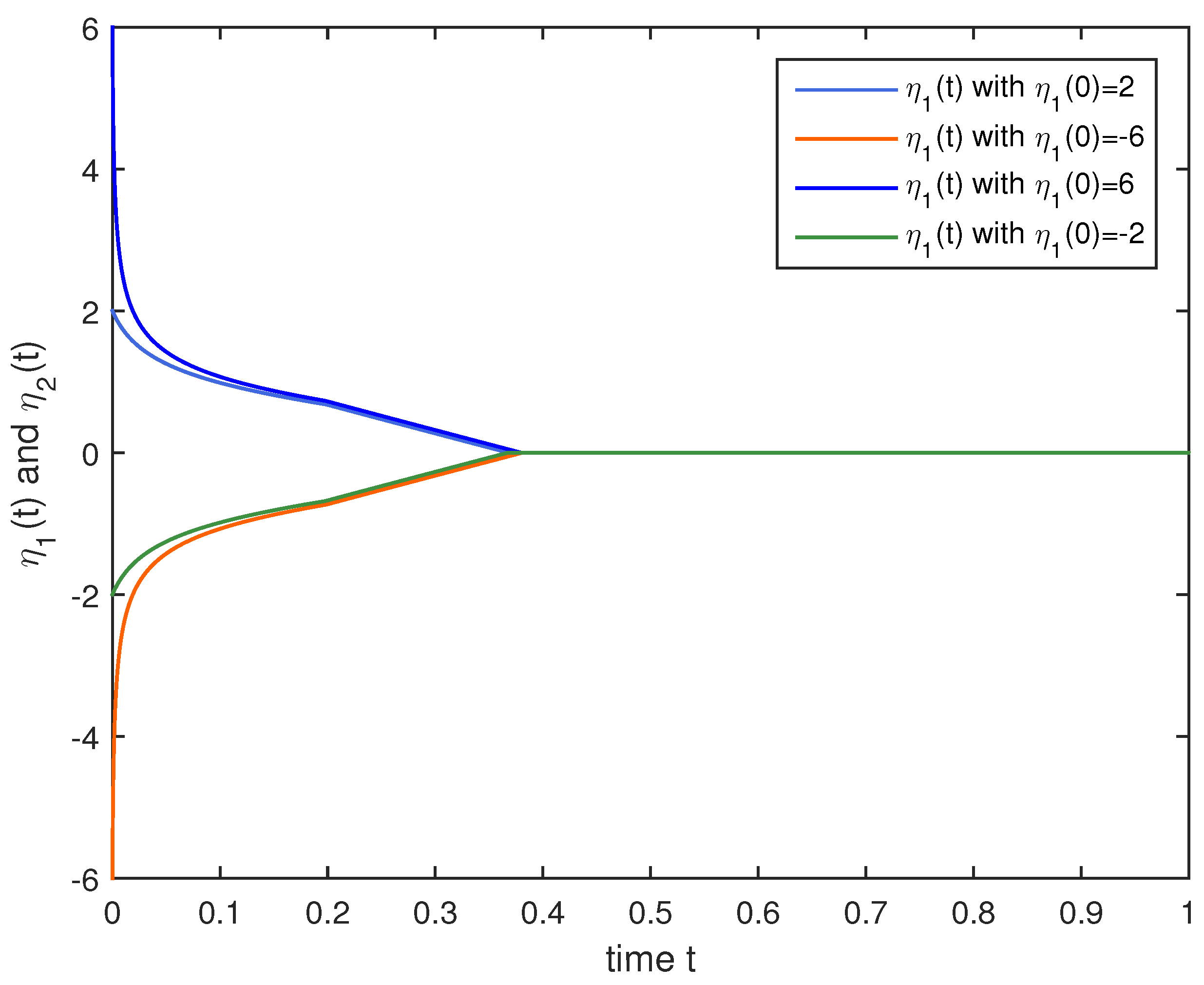
4. Numerical Simulations

In this section, we provide two examples to demonstrate the validity of the theoretical results in Section 3.

Example 1.

The ball motion model we considered is described as follows:

$$\dot{u}=a\left(t\right)\mathrm{sign}(u\left(t\right)-a)+b(t,u(t\left)\right)b\left(t\right),t\ge 0,$$

(29)

where $u\left(t\right)$ represents the velocity of a ball and the positive constant a is a threshold value of velocity. The function $a\left(t\right)$ represents the effect of external factors on the trajectory of the ball and discontinuous function $b(t,u(t\left)\right)$ defines a speed controller. If we chose

$$a\left(t\right)=\frac{2}{1+t^2}-\frac{t}{2}|cost|,$$

(30)

$$b(t,u(t\left)\right)=(-\frac{2}{1+t^2}-\frac{3}{8}){(u\left(t\right)-a)}^{2+2\mathrm{sign}({(u\left(t\right)-a)}^2-1)}\mathrm{sign}(u\left(t\right)-a),$$

(31)

and select the Lyapunov functional as

$$\mathcal{U}(t,u\left(t\right))={(u\left(t\right)-a)}^2,$$

(32)

then $\dot{\mathcal{U}}\le (\frac{4}{1+t^2}-t|cost|){\mathcal{U}}^{\frac{1}{2}}+(-\frac{4}{1+t^2}-\frac{3}{4}){\mathcal{U}}^{\frac{3}{2}+\mathrm{sign}({(u\left(t\right)-a)}^2-1)}$. It then follows from Theorem 3 that the conditions are fulfilled with $l\left(t\right)=\frac{4}{1+t^2}-t|cost|$, $r\left(t\right)=-\frac{4}{1+t^2}-\frac{3}{4}$, $\alpha =\frac{1}{2}$, $\gamma =\frac{3}{2}$, ${\lambda }_1=\frac{1}{2}$. Assume $a=30(m/s)$, and choose six different initial values as $u_0=20(m/s)$, $u_0=22(m/s)$, $u_0=25(m/s)$, $u_0=28(m/s)$, $u_0=31(m/s)$, $u_0=33(m/s)$, $u_0=35(m/s)$ and $u_0=38(m/s)$, then we can see the trajectories of the velocity with different initial values $u_0$ converge to 30 in fixed-time from Figure 1 and the ST $T=2.894\le T_{max}=3.5556$.

Example 2.

Consider the following discontinuous neural network and investigate its fixed-time stability by selecting appropriate external input, where $-\frac{1}{2}cost$ is the self-inhibition; $z_i\left(s\right)=tanh\left(s\right)+\mathrm{sign}s(i=1,2)$ represent activation functions; $u_1\left(t\right)$ and $u_2\left(t\right)$ are external inputs:

$$\begin{array}{c}\hfill \left\{\begin{array}{cc}\hfill {\dot{\eta }}_1\left(t\right)& =-\frac{1}{2}{\eta }_1\left(t\right)cost+\frac{1}{1+t}{z}_1\left({\eta }_1\left(t\right)\right)+u_1\left(t\right),\hfill \\ \hfill {\dot{\eta }}_2\left(t\right)& =-\frac{1}{2}{\eta }_2\left(t\right)cost+\frac{1}{1+\sqrt{t}}{z}_2\left({\eta }_2\left(t\right)\right)+u_2\left(t\right).\hfill \end{array}\right.\end{array}$$

(33)

Recourse to differential inclusion theory, from system (33)

$$\begin{array}{c}\hfill \left\{\begin{array}{cc}\hfill {\dot{\eta }}_1\left(t\right)& \in -\frac{1}{2}{\eta }_1\left(t\right)cost+\frac{1}{1+t}\overline{co}\left(z_1\left({\eta }_1\left(t\right)\right)\right)+u_1\left(t\right),\hfill \\ \hfill {\dot{\eta }}_2\left(t\right)& \in -\frac{1}{2}{\eta }_2\left(t\right)cost+\frac{1}{1+\sqrt{t}}\overline{co}\left(z_2\left({\eta }_2\left(t\right)\right)\right)+u_2\left(t\right).\hfill \end{array}\right.\end{array}$$

(34)

Similarly, there exists ${\varsigma }_1\left(t\right)\in \overline{co}\left(z_1\left({\eta }_1\left(t\right)\right)\right)$ and ${\varsigma }_2\left(t\right)\in \overline{co}\left(z_2\left({\eta }_2\left(t\right)\right)\right)$ for a.e. t, ${\varsigma }_i\left(t\right)$ satisfy ${\varsigma }_i\left(t\right)\le \left|{\eta }_i\left(t\right)\right|+1,i=1,2$, such that

$$\begin{array}{c}\hfill \left\{\begin{array}{cc}\hfill {\dot{\eta }}_1\left(t\right)& =-\frac{1}{2}{\eta }_1\left(t\right)cost+\frac{1}{1+t}{\varsigma }_1\left(t\right)+u_1\left(t\right),\hfill \\ \hfill {\dot{\eta }}_2\left(t\right)& =-\frac{1}{2}{\eta }_2\left(t\right)cost+\frac{1}{1+\sqrt{t}}{\varsigma }_2\left(t\right)+u_2\left(t\right).\hfill \end{array}\right.\end{array}$$

(35)

$\eta \left(t\right)=0$ is the trivial solution of (35) when $u_1\left(t\right)=u_2\left(t\right)=0$. Select the initial values as ${\eta }_0={(3,-1)}^T$, ${\eta }_0={(-3,1)}^T$. We derive the solution trajectory of system (35), which is depicted in Figure 2. As can be seen, the solution trajectory of system (35) can not converge to zero. In order to achieve the FXTS, the following external inputs are given:

$$\begin{array}{cc}\hfill u_1\left(t\right)=& \frac{1}{2}{\eta }_1\left(t\right)cost-\frac{1}{1+t}{\eta }_1\left(t\right)-\frac{1}{1+t}\mathrm{sign}\left({\eta }_1\left(t\right)\right)+(\frac{1}{1+t^2}-\frac{t|cost|}{2}){\left|{\eta }_1\left(t\right)\right|}^{\frac{1}{5}}\mathrm{sign}\left({\eta }_1\left(t\right)\right)\hfill \\ \hfill & -(\frac{4}{1+t^2}+4){\left|{\eta }_1\left(t\right)\right|}^{\frac{11}{5}+2\mathrm{sign}({\eta }_1^2\left(t\right)+{\eta }_2^2\left(t\right)-1)}\mathrm{sign}\left({\eta }_1\left(t\right)\right),\hfill \end{array}$$

(36)

$$\begin{array}{cc}\hfill u_2\left(t\right)=& \frac{1}{2}{\eta }_2\left(t\right)cost-\frac{1}{1+\sqrt{t}}{\eta }_2\left(t\right)-\frac{1}{1+t}\mathrm{sign}\left({\eta }_2\left(t\right)\right)+(\frac{1}{1+t^2}-\frac{t|cost|}{2}){\left|{\eta }_2\left(t\right)\right|}^{\frac{1}{5}}\mathrm{sign}\left({\eta }_2\left(t\right)\right)\hfill \\ \hfill & -(\frac{4}{1+t^2}+4){\left|{\eta }_2\left(t\right)\right|}^{\frac{11}{5}+2\mathrm{sign}({\eta }_1^2\left(t\right)+{\eta }_2^2\left(t\right)-1)}\mathrm{sign}\left({\eta }_2\left(t\right)\right).\hfill \end{array}$$

(37)

The Lyapunov function is selected as $\mathcal{U}(t,\eta \left(t\right))={\eta }_1^2\left(t\right)+{\eta }_2^2\left(t\right)$, then $\dot{\mathcal{U}}\left(t\right)\le (\frac{2^{\frac{7}{5}}}{1+t^2}-t|cost|){\mathcal{U}}^{\frac{3}{5}}\left(t\right)-(\frac{2^{\frac{7}{5}}}{1+t^2}\left(t\right)+2^{\frac{7}{5}}){\mathcal{U}}^{\frac{8}{5}+\mathrm{sign}(\mathcal{U}-1)}\left(t\right)$, where $l\left(t\right)=\frac{2^{\frac{7}{5}}}{1+t^2}-t|cost|$, $r\left(t\right)=-\frac{2^{\frac{7}{5}}}{1+t^2}$$-2^{\frac{7}{5}}$, $\alpha =\frac{3}{5}$, $\gamma =\frac{8}{5}$. We see that $l\left(t\right)$ is indefinite and $r\left(t\right)$, $l^{+}\left(t\right)+r\left(t\right)$ are negative, ${\lambda }_1=2^{\frac{7}{5}}$, the ST T satisfies $T=0.2681\le T_{max}=1.1841$. After that, it is clear that all the conditions in Theorem 3 are satisfied by utilizing the external inputs we have designed. In addition, the solution trajectories of system (35) with inputs (36) and (37) are pictured by Figure 3. Obviously, the state could converge to 0 in fixed-time.

To demonstrate that our estimate of ST in Corollary 1 is better than that in [33], consider system (35) with the following inputs:

$$\begin{array}{cc}\hfill u_1\left(t\right)=& \frac{1}{2}{\eta }_1\left(t\right)cost-\frac{1}{1+t}{\eta }_1\left(t\right)-\frac{1}{1+t}\mathrm{sign}\left({\eta }_1\left(t\right)\right)-2\mathrm{sign}\left({\eta }_1\left(t\right)\right)\hfill \\ \hfill & -2|{\eta }_1{\left(t\right)|}^{2+2\mathrm{sign}({\eta }_1^2\left(t\right)+{\eta }_2^2\left(t\right)-1)}\mathrm{sign}\left({\eta }_1\left(t\right)\right),\hfill \end{array}$$

(38)

$$\begin{array}{cc}\hfill u_2\left(t\right)=& \frac{1}{2}{\eta }_2\left(t\right)cost-\frac{1}{1+\sqrt{t}}{\eta }_2\left(t\right)-\frac{1}{1+t}\mathrm{sign}\left({\eta }_2\left(t\right)\right)-2\mathrm{sign}\left({\eta }_2\left(t\right)\right)\hfill \\ \hfill & -2|{\eta }_2{\left(t\right)|}^{2+2\mathrm{sign}({\eta }_1^2\left(t\right)+{\eta }_2^2\left(t\right)-1)}\mathrm{sign}\left({\eta }_2\left(t\right)\right).\hfill \end{array}$$

(39)

The Lyapunov function and initial values are selected as $\mathcal{U}(t,\eta \left(t\right))={\eta }_1^2\left(t\right)+{\eta }_2^2\left(t\right)$, ${\eta }_0={(2,-6)}^T$, ${\eta }_0={(-6,2)}^T$, respectively. Then $\dot{\mathcal{U}}\left(t\right)\le -4{\mathcal{U}}^{\frac{1}{2}}\left(t\right)-4{\mathcal{U}}^{\frac{3}{2}+\mathrm{sign}\mathcal{U}-1}\left(t\right)$, and it satisfies the conditions in Corollary 1 with $l=r=-4$, $\alpha =\frac{1}{2}$, $\gamma =\frac{3}{2}$. Denote $T_{max}$ in Corollary 1 and [33] as $T_{max}^1$ and $T_{max}^2$, after calculation, we obtain $T=0.3715<T_{max}^1=0.4167<$$T_{max}^2=0.7667$. The solution trajectories of system (35) with inputs (38) and (39) are pictured by Figure 4.

Remark 8.

In fact, the external inputs (36) and (37) used in Example 2 play important roles in achieving FXTS, and each part of them has a specific role. We can see that $-\frac{1}{2}{\eta }_1\left(t\right)cost+\frac{1}{1+t}{\varsigma }_1\left(t\right)$ and $-\frac{1}{2}{\eta }_2\left(t\right)cost+\frac{1}{1+\sqrt{t}}{\varsigma }_2\left(t\right)$ in system (35) are compensated by the terms $\frac{1}{2}{\eta }_i\left(t\right)cost$, $-\frac{1}{1+t}\mathrm{sign}\left({\eta }_i\left(t\right)\right)$ (i = 1,2), $-\frac{1}{1+t}{\eta }_1\left(t\right)$ and $-\frac{1}{1+\sqrt{t}}{\eta }_2\left(t\right)$. What is more, we introduce the terms $(\frac{1}{1+t^2}-\frac{t|cost|}{2}){\left|{\eta }_i\left(t\right)\right|}^{\frac{1}{5}}\mathrm{sign}\left({\eta }_i\left(t\right)\right)$, $-(\frac{4}{1+t^2}+4){\left|{\eta }_i\left(t\right)\right|}^{\frac{11}{5}+2\mathrm{sign}({\eta }_1^2\left(t\right)+{\eta }_2^2\left(t\right)-1)}\mathrm{sign}\left({\eta }_i\left(t\right)\right)$ (i = 1,2) to guarantee that the neural network achievese FXTS.

5. Conclusions

We established some novel FNTS/FXTS Lyapunov theorems for the trivial solution for DI (2) based on the Filippov solution and Lyapunov stability theory. Several sufficient conditions for estimating the ST were proposed. The results could be easily verified by numerical simulations. It was shown that the estimation of ST in Corollary 1 was more accurate than that in [33]. Moreover, the results in our paper were more general than that in [11,31,32,33] as the coefficients in the inequalities satisfied by the general LF could be time-varying functions and not all coefficients needed to be negative. To extend the main achievements of this paper, some topics could be further considered, such as FNTS/FXTS with impulsive effects and finite/fixed-time synchronization.

References

1. Hong, Y.; Jiang, Z.; Feng, G. Finite-time input-to-state stability and applications to finite-time control design. SIAM J. Control Optim. 2010, 48, 4395–4418. [Google Scholar] [CrossRef]
2. Nersesov, S.G.; Haddad, W.M. Finite-time stabilization of nonlinear impulsive dynamical systems. Nonlinear Anal. Hybrid Syst. 2008, 2, 832–845. [Google Scholar] [CrossRef]
3. Bhat, S.; Bernstein, D. Finite-Time stability of continuous autonomous systems. SIAM J. Control Optim. 2000, 38, 751–766. [Google Scholar] [CrossRef]
4. Xi, Q.; Liang, Z.; Li, X. Uniform finite-time stability of nonlinear impulsive time-varying systems. Appl. Math. Model. 2021, 91, 913–922. [Google Scholar] [CrossRef]
5. Wang, L.; Sun, S.; Xia, C. Finite-time stability of multi-agent system in disturbed environment. Nonlinear Dyn. 2012, 67, 2009–2016. [Google Scholar] [CrossRef]
6. Wang, Y.; Shi, X.; Wang, G.; Zuo, Z. Finite-time stability for continuous-time switched systems in the presence of impulse effects. IET Control Theory Appl. 2012, 6, 1741–1744. [Google Scholar] [CrossRef]
7. Orlov, Y. Finite Time Stability and Robust Control Synthesis of Uncertain Switched Systems. SIAM J. Control Optim. 2005, 43, 1253–1271. [Google Scholar] [CrossRef]
8. Yang, X.; Cao, J. Finite-time stochastic synchronization of complex networks. Appl. Math. Model. 2010, 34, 3631–3641. [Google Scholar] [CrossRef]
9. Chen, G.; Yang, Y. Finite-time stability of switched nonlinear time-varying systems via indefinite Lyapunov functions. Int. J. Robust Nonlinear Control 2018, 28, 1901–1912. [Google Scholar] [CrossRef]
10. Xu, J.; Sun, J. Finite-time stability of linear time-varying singular impulsive systems. IET Control Theory Appl. 2010, 4, 2239–2244. [Google Scholar] [CrossRef]
11. Polyakov, A. Nonlinear feedback design for fixed-time stabilization of linear control systems. IEEE Trans. Autom. Control 2012, 57, 2106–2110. [Google Scholar] [CrossRef] [Green Version]
12. Defoort, M.; Polyakov, A.; Demesure, G.; Djemai, M. Leader-follower fixed-time consensus for multi-agent systems with unknown non-linear inherent dynamics. IET Control Theory Appl. 2015, 9, 2165–2170. [Google Scholar] [CrossRef] [Green Version]
13. Ni, J.; Liu, L.; Liu, C.; Hu, X.; Li, S. Fast fixed-time nonsingular terminal sliding mode control and its application to chaos suppression in power system. IEEE Trans. Circuits Syst. Express Briefs 2017, 64, 151–155. [Google Scholar] [CrossRef]
14. Chen, C.; Sun, Z. Fixed-time stabilisation for a class of high-order non-linear systems. IET Control Theory Appl. 2018, 12, 2578–2587. [Google Scholar] [CrossRef]
15. Yu, J.; Yu, S.; Li, J.; Yan, Y. Fixed-time stability theorem of stochastic nonlinear systems. Int. J. Control 2019, 92, 2194–2200. [Google Scholar] [CrossRef]
16. Hu, J.; Sui, G.; Lv, X.; Li, X. Fixed-time control of delayed neural networks with impulsive perturbations. Nonlinear-Anal.-Model. Control 2018, 23, 904–920. [Google Scholar] [CrossRef] [Green Version]
17. Cai, Z.; Huang, L.; Zhang, L. Finite-time synchronization of master-slave neural networks with time-delays and discontinuous activations. Appl. Math. Model. 2017, 47, 208–226. [Google Scholar] [CrossRef]
18. Wang, Z.; Cao, J.; Cai, Z.; Abdel-Aty, M. A novel Lyapunov theorem on finite/fixed-time stability of discontinuous impulsive systems. Chaos 2020, 30, 013139. [Google Scholar] [CrossRef]
19. Cai, Z.; Zhu, M.; Huang, L.; Wang, D. Finite-time stabilization control of memristor-based neural networks. Nonlinear Anal. Hybrid Syst. 2016, 20, 37–54. [Google Scholar] [CrossRef]
20. Wang, D.; Huang, L.; Cai, Z. On the periodic dynamics of a general Cohen-Grossberg BAM neural networks via differential inclusions. Neurocomputing 2013, 118, 203–214. [Google Scholar] [CrossRef]
21. Wang, D.; Huang, L. Periodicity and global exponential stability of generalized Cohen-Grossberg neural networks with discontinuous activations and mixed delays. Neural Netw. 2014, 51, 80–95. [Google Scholar] [CrossRef] [PubMed]
22. Guo, Z.; Huang, L. Generalized Lyapunov method for discontinuous systems. Nonlinear Anal. Theory Methods Appl. 2009, 71, 3083–3092. [Google Scholar] [CrossRef]
23. Filipov, A.F. Differential Equations with Discontinuous Right-Hand Side; Kluwer Academic Press: Dordrecht, The Netherlands, 1988. [Google Scholar]
24. Kim, S.J.; Ha, I.J. Existence of Carathe/spl acute/odory solutions in nonlinear systems with discontinuous switching feedback controllers. IEEE Trans. Autom. Control 2004, 49, 1167–1171. [Google Scholar] [CrossRef]
25. Hu, C.; Yu, J.; Chen, Z.; Jiang, H.; Huang, T. Fixed-time stability of dynamical systems and fixed-time synchronization of coupled discontinuous neural networks. Neural Netw. 2017, 89, 74–83. [Google Scholar] [CrossRef]
26. Ding, Z.; Zeng, Z.; Wang, L. Robust Finite-Time Stabilization of Fractional-Order Neural Networks with Discontinuous and Continuous Activation Functions Under Uncertainty. IEEE Trans. Neural Networks Learn. Syst. 2018, 29, 1477–1490. [Google Scholar] [CrossRef]
27. Cai, Z.; Huang, L.; Wang, Z. Finite/Fixed-Time stability of nonautonomous functional differential inclusion: Lyapunov approach involving indefinite derivative. IEEE Trans. Neural Networks Learn. Syst. 2021. Early Access. [Google Scholar] [CrossRef] [PubMed]
28. Clarke, F. Optimization and Nonsmooth Analysis; Wiley Press: Hoboken, NJ, USA, 1983. [Google Scholar]
29. Kong, F.; Zhu, Q.; Huang, T. Fixed-Time Stability for Discontinuous Uncertain Inertial Neural Networks with Time-Varying Delays. IEEE Trans. Syst. Man Cybern. Syst. 2021, 52, 4507–4517. [Google Scholar] [CrossRef]
30. Hardy, G.H.; Littlewood, J.E.; Polya, G. Inequalities; Cambridge University Press: Cambridge, UK, 1988. [Google Scholar]
31. Parsegov, S.E.; Polyakov, A.E.; Shcherbakov, P. Nonlinear fixed-time control protocol for uniform allocation of agents on a segment. Dokl. Math. Vol. 2013, 87, 133–136. [Google Scholar] [CrossRef]
32. Zuo, Z.; Tie, L. Distributed robust finite-time nonlinear consensus protocols for multi-agent systems. Int. J. Syst. Sci. 2016, 47, 1366–1375. [Google Scholar] [CrossRef]
33. Li, N.; Wu, X.; Yang, Q. Fixed-Time Synchronization of Complex Dynamical Network with Impulsive Effects. IEEE Access 2020, 8, 33072–33079. [Google Scholar] [CrossRef]
34. Wang, Z.; Cao, J.; Cai, Z.; Huang, L. Periodicity and fixed-time periodic synchronization of discontinuous delayed quaternion neural networks. J. Frankl. Inst. Eng. Appl. Math. 2020, 357, 4242–4271. [Google Scholar] [CrossRef]
Figure 1. Trajectories of the velocity u ( t ) in Example 1.
Mathematics 10 02221 g001
Figure 2. State−trajectories without externalcontrol input in Example 2.
Mathematics 10 02221 g002
Figure 3. State−trajectories with external inputs (36) and (37).
Mathematics 10 02221 g003
Figure 4. State−trajectories with external inputs (38) and (39).
Mathematics 10 02221 g004
Publisher’s Note: MDPI stays neutral with regard to jurisdictional claims in published maps and institutional affiliations.