Permutation Tests for Metaheuristic Algorithms

Abstract

Many metaheuristic approaches are inherently stochastic. In order to compare such methods, statistical tests are needed. However, choosing an appropriate test is not trivial, given that each test has some assumptions about the distribution of the underlying data that must be true before it can be used. Permutation tests (P-Tests) are statistical tests with minimal number of assumptions. These tests are simple, intuitive and nonparametric. In this paper, we argue researchers in the field of metaheuristics to adopt P-Tests to compare their algorithms. We define two statistic tests and then present an algorithm that uses them to compute the p-value. The proposed process is used to compare 5 metaheuristic algorithms on 10 benchmark functions. The resulting p-values are compared with the p-values of two widely used statistical tests. The results show that the proposed P-test is generally consistent with the classical tests, but more conservative in few cases.

1. Introduction

Many optimization problems can be defined as follows,

$$\begin{array}{c}\hfill \min f\left(x\right),\\ \hfill s.t.x\in \mathcal{S}\end{array}$$

(1)

where x is a candidate solution to the given optimization problem (we use the boldface to indicate vectors), i.e., a D-dimensional vector $x=(x_1,x_2,\dots ,x_D)$ where each $x_i$ is a variable, $f\left(·\right)$ is the objective function (that we assume, without loss of generality, to be minimized), and $\mathcal{S}$ is the search space domain, that in bound-constrained optimization is a hyper-rectangle defined by lower and upper bounds, respectively $l=(l_1,l_2,\dots ,l_D)$ and $u=(u_1,u_2,\dots ,u_D)$, s.t., $l_i\le x_i\le u_i\forall i\in \{1,2,\dots ,D\}$.

Most classic algorithms that try to solve the above problem are deterministic and may require gradient information such as the well-known Newton–Raphson method. If the function is not differentiable, nongradient algorithms such as Nelder–Mead are preferred [1].

Stochastic optimization algorithms, on the other hand, have two types: heuristic and metaheuristic. Heuristic means to discover by trial and error. Heuristic methods may find the optimal solution to an optimization problem but there is no guarantee for this. Hence, they work most but not all of the time.

Heuristic algorithms are typically problem-dependent but metaheuristic algorithms are high-level, problem-independent frameworks. These algorithms produce acceptable solutions to complex problems in a reasonable time.

Examples of well-known metaheuristic approaches are Ant Colony Optimization (ACO) [2], Particle Swarm Optimization (PSO) [3] and Differential Evolution (DE) [4].

Some recent noteworthy examples of metaheuristic algorithms include, but are not limited to:

• Novel bio-inspired algorithms (e.g., the Harris hawks optimization algorithm [5], the slime mould algorithm [6], the Multi-Verse Algorithm [7]);
• Variations of existing techniques, such as variants of the Flower Pollination algorithm [8], PSO [9,10,11], or DE [12,13,14];
• Hybrid algorithms obtained by combining for instance ACO with chaotic sequences [15] and PSO with local solvers [16].

Many of the newly proposed metaheuristics lacked novelty. They often reiterate ideas introduced in older metaheuristics such as PSO, but using new natural metaphors. This created something like a “metaphor bubble” in the area of metaheuristics. For more details, please refer to [17,18]. Therefore, the results of an algorithm should be validated using appropriate statistical tests. Parametric tests such as t-tests cannot be used without ensuring that the assumptions (e.g., the normality assumption for the results) required for those tests are met by the obtained results. Nonparametric tests such as Wilcoxon’s test [19] do not assume particular characteristics for the underlying data distribution. Thus, if the assumptions of parametric tests do not hold or are not checked, nonparametric tests should be used. However, nonparametric tests are less powerful than parametric tests [20]. Nevertheless, the parametric tests’ assumption often fails to hold when comparing the results of metaheuristic algorithms. Consequently, nonparametric tests should be used [21]. The recommendation is to use Wilcoxon’s test to compare the performance of two metaheuristic algorithms [21].

Once the p-values are calculated using the appropriate statistical test, a correction method (e.g., Bonferroni–Dunn [22]) must be used to counteract the effect of multiple comparisons, by controlling either the family-wise error rate, or the false discovery error rate [23].

Permutation tests [24] are nonparametric tests that are very simple, intuitive and require very few assumptions. Thus, in many bioinformatics applications, for example, where there is no evidence to assume normality, the nonparametric permutation tests are a widely used technique [25]. This lack of normality assumption also applies to the field of metaheuristics. This is why in this paper, we propose using it to compute statistical significance.

The paper is organized as follows: Section 2 explains permutation tests along with an illustrating example. The approach to use permutation tests to compare the performance of two metaheuristic approaches is presented in Section 3. Experimental results are discussed in Section 4. Section 5 concludes the paper.

2. Permutation Tests (P-Tests)

Permutation tests [24] are general, nonparametric and computationally fool-proof way to prove significance [26]. If a hypothesis is supported by the real data, a new data set constructed by randomly shuffling the original data should be less likely to support the hypothesis.

To use P-tests, a statistic reflecting the hypothesis about the data should be defined. For example, if we want to discover if there is a correlation between gender and height, a possible statistic is the difference between the mean height of men and women [26].

Once a test statistic has been defined, the statistic is calculated for the original data. For our height–gender example, the difference between the mean height of men and women is computed. Let us call that difference d.

Then, the real data are randomly shuffled (i.e., permuted). In our example, a new data set is constructed by randomly assigning gender to the original outcome variables. Then, the statistic is computed for the shuffled data and it is recorded. This process is repeated N times. Now, we have a distribution of statistics produced by the N random permutations.

The rank of the test statistics on the actual data (i.e., d) among the distribution of statistic values resulting from the N random permutations determines the p-value. More specifically, p-value is the number of statistic values more extreme than (or as extreme as) d divided by $N+1$.

Figure 1a shows that the real statistic value, d, (as a vertical dashed line) lies on the right of the distribution, demonstrating a significant difference. Contrast this with Figure 1b, where d lies in the middle of the distribution (i.e., no significant difference).

The accuracy of P-tests depends on the number of permutations, N, which should be $\left(\genfrac{}{}{0pt}{}{2n}{n}\right)$, where n is the sample size. It is clear that N is extremely large even for very modest sample sizes. Thus, P-tests can be computationally very intensive. Some studies have tried to investigate reducing the number of permutations (e.g., [25,27]). In practice, we typically randomly sample a large number of permutations from the total number that are available. The resulting test is no longer “exact”, but we can make it as accurate as we wish by choosing a suitable number of random permutations. The more, the better. When we use a sample of all possible permutations, the resulting test is referred to as a randomization test.

In this paper, we will focus on the primitive form of P-tests (i.e., randomization tests), which can be implemented by anyone with basic programming skills.

Example

An example of how P-tests work is adopted from https://www.r-bloggers.com/2019/04/what-is-a-permutation-test/ (accessed on February 2022) with slight modifications.

Suppose that two students, Jane and John, sit a pre-semester test and a final exam. The students’ scores are shown in

Table 1. Student score example.

Exam	Jane	John	(Sample) Average
Pre-Semester Test:	70	75	72.5
Final Exam:	76	72	74.0

.

Based on this very small sample, we are interested in whether the course improves students’ knowledge of the course material. Let the null hypothesis be that there is no improvement in knowledge and let the test statistic be the difference between the “after” and “before” sample average scores. Then, d = (74.0 – 72.5) = 1.5.

Given that there are 4 scores in Table 1, and the 2 scores associated with the pre-semester test can be assigned in $4!/(2!2!)=6$ ways (i.e., $N=6$). The 6 possible permutations are listed in

Table 2. Permutation possibilities based on the students scores where “P” and “F” refer to the pre-semester test and final exam.

Permutation i	70	72	75	76	${\mathit{d}}_{\mathit{i}}$
1	P	P	F	F	4.5
2	P	F	P	F	1.5 (d)
3	P	F	F	P	0.5
4	F	P	P	F	−0.5
5	F	P	F	P	−1.5
6	F	F	P	P	−4.5

.

The p-value is then calculated as $2/6=0.333$ (which is the fraction of the 6 $d_i$ values greater than or equal to d). If the significance level, $\alpha$, is 0.05, we cannot reject the null hypothesis and we can say that there is no evidence that the course led to improvement in students’ knowledge.

3. P-Tests for Metaheuristics

In this section, we will show how P-tests can be used in the context of comparing metaheuristic algorithms.

First, let us check if P-tests can be used to compare metaheuristics. The main assumption of a P-test is the exchangeability of the data (i.e., shuffling the observed data points keeps the data-set just as likely as the original one). To be more precise, this means that the distribution of the test statistic under the null hypothesis must be invariant to any permutation of the data. This is valid when comparing metaheuristic algorithms since each metaheuristic is applied to a problem n times generating n objective function values. To compare two algorithms, we will have $2n$ values that are exchangeable.

Second, a test statistic should be defined. Usually, it is the difference between the means. However, since the distribution of the objective function values are generally not normally distributed, we will use the medians instead of the means. This will be more consistent with the recommendations of using nonparametric tests when comparing metaheuristic methods [20]. In addition, we will use the absolute value of the differences between the medians since we are interested in finding if there is a significant difference between two algorithms. Thus, our test statistic, d, is defined as

$$d=\left|m_A-m_B\right|$$

(2)

where $m_A$ and $m_B$ are the median values of the n objective function values for metaheuristic A and B, respectively.

Finally, the P-test is applied according to Algorithm 1. The Algorithm takes two data sets $S_A$ and $S_B$ representing the n best objective function values obtained by metaheurisitc methods A and B, respectively. The test statistic, d, is then computed. The two sets are merged and randomly shuffled. The shuffled data set is divided into two data sets, $S_A^{\prime }$ and $S_B^{\prime }$, of size n each. The test statistic is re-computed and saved. This is repeated N times and a distribution of N statistics is generated. Finally, the rank of d within the distribution is determined and the p-value is calculated.

Figure 2 shows the P-test implemented using the Wolfram Language. A Python implementation is available at https://github.com/i0mar/Permutation-Test-for-Metaheuristics (accessed on February 2022).

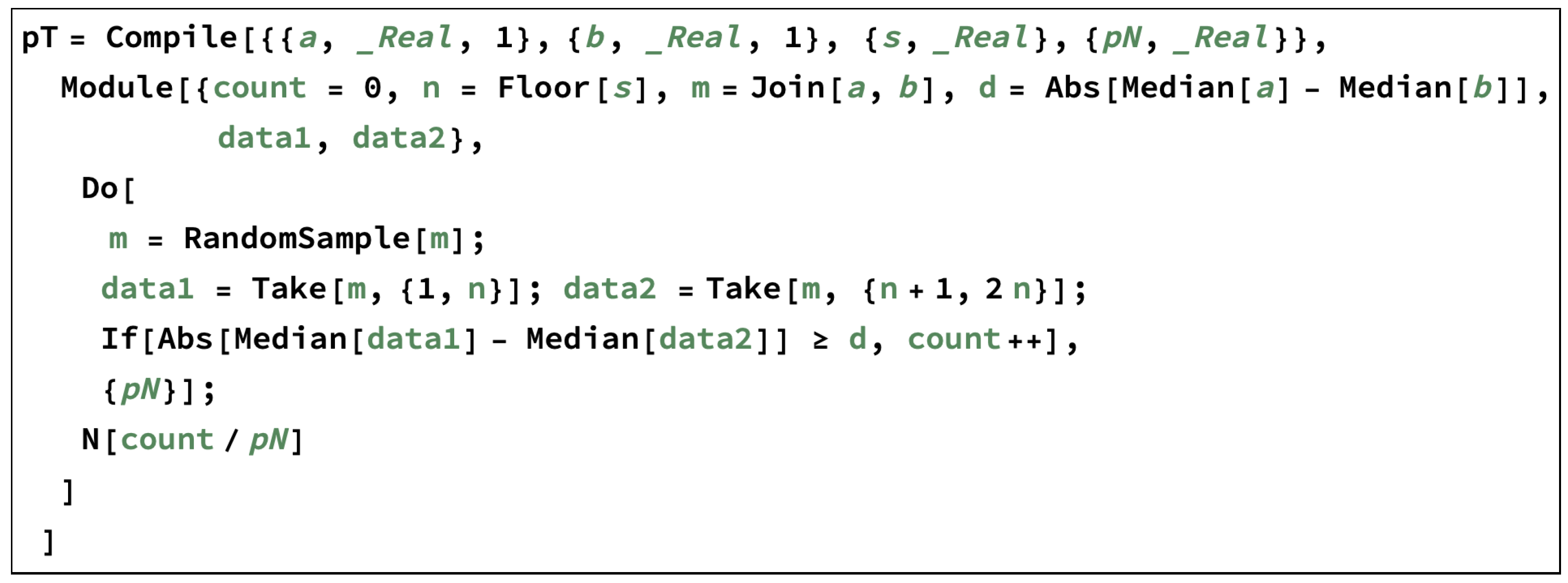
Algorithm 1 P-test for two algorithms

Inputs: $n_A$ best solutions obtained by Alg. A ($S_A$), and $n_B$ best solutions obtained by Alg. B ($S_B$) (in our case $n_A=n_B$). The number of permutations generated, N. Compute the median of $S_A$ and save it as $m_A$ and the median of $S_B$ and saved it as $m_B$. Compute the absolute difference between $m_A$ and $m_B$ and save it as d using Equation (2). while$i<N$  do     Merge the two lists $S_A$ and $S_B$ into one list S.     Randomly permute S.     Partition S into two lists $S_A^{\prime }$ (of size $n_A$) and $S_B^{\prime }$ (of size $n_B$).     Compute the median of $S_A^{\prime }$ and $S_B^{\prime }$ and save them as $m_A^{\prime }$ and $m_B^{\prime }$.     Compute the difference between $m_A^{\prime }$ and $m_B^{\prime }$ and save it as $d_i$ using Equation (2).     $i:=i+1$. end while Count the $d_i$’s that are more extreme than d (i.e., $d_i\ge d$) and save it as c. Compute the p-value as $c/(N+1)$.

4. Experimental Results

In this section, we will investigate the use of the proposed P-test as a statistical test to compare the performance of different metaheuristic approaches. Five representative approaches have been chosen:

• Honey Badger Algorithm (HBA) [28];
• Jaya [29];
• Jellyfish Search (JS) [30];
• SHADE [31]; and
• L-SHADE [12].

Simply put, Jaya is a very simple metaheuristic approach, HBA and JS are very recent metaphor-based metaheuristics, while SHADE and L-SHADE are state-of-the-art methods. The five approaches are tested on the 10 benchmark functions used at the CEC 2020 competition on single objective bound-constrained numerical optimization [32].

Table 3. Summary of the CEC 2020 benchmark functions.

Function	Type	Optimum Value
F1	Unimodal function	100
F2	Basic function	1100
F3	Basic function	700
F4	Basic function	1900
F5	Hybrid function	1700
F6	Hybrid function	1600
F7	Hybrid function	2100
F8	Composition function	2200
F9	Composition function	2400
F10	Composition function	2500

summarizes the 10 CEC 2020 benchmark functions. The first four functions are shifted and rotated well-known functions. The next three functions are hybrid, which means they are linear combinations of several basic functions. Finally, the last three functions are compositions, i.e., couplings between the previous functions considered in different parts of their optimization domains. All functions are scalable, which means that they can be computed for different numbers of problem dimensions D. Accordingly, the search range for all functions is ${[-100,100]}^D$. In our experiments, we set D to 20. The mathematical description of each function can be found in [32].

Each of the compared algorithms was executed for 50 independent runs (i.e., n = 50) using 50,000 function evaluations. The pseudo random number generator used is the default random generator for the NumPy Package in Python, using a seed of 123,456,789.

4.1. Descriptive Statistics and Plots

The detailed statistics of HBA, Jaya, JS, SHADE, and L-SHADE, in terms of median, mean, standard deviation (SD), minimum (i.e., best), and maximum (i.e., worst) objective function values (across the best function values obtained at the end of the allotted budget in all the available runs for each problem) on the CEC 2020 benchmark functions are reported in

Table 4. The CEC 2020 ($D=20$) function values achieved by HBA over 50 runs and 50,000 function evaluations.

Function	Median	Mean	SD	Min	Max
F1	3.65E + 03	3.95E + 03	2.94E + 03	1.00E + 02	9.28E + 03
F2	2.69E + 03	2.73E + 03	6.18E + 02	1.68E + 03	4.55E + 03
F3	7.83E + 02	7.86E + 02	1.83E + 01	7.52E + 02	8.39E + 02
F4	1.90E + 03	1.90E + 03	1.93E + 00	1.90E + 03	1.91E + 03
F5	5.86E + 04	6.52E + 04	3.84E + 04	5.43E + 03	1.95E + 05
F6	1.80E + 03	1.80E + 03	0.00E + 00	1.80E + 03	1.80E + 03
F7	1.83E + 04	4.13E + 04	1.46E + 05	3.69E + 03	1.06E + 06
F8	2.30E + 03	2.62E + 03	9.36E + 02	2.30E + 03	7.07E + 03
F9	2.91E + 03	2.95E + 03	9.99E + 01	2.84E + 03	3.25E + 03
F10	2.96E + 03	2.96E + 03	3.51E + 01	2.90E + 03	3.02E + 03

,

Table 5. The CEC 2020 ($D=20$) function values achieved by Jaya over 50 runs and 50,000 function evaluations.

Function	Median	Mean	SD	Min	Max
F1	2.20E + 09	2.28E + 09	4.85E + 08	1.43E + 09	3.83E + 09
F2	4.93E + 03	4.87E + 03	3.49E + 02	4.01E + 03	5.61E + 03
F3	8.88E + 02	8.92E + 02	1.80E + 01	8.61E + 02	9.40E + 02
F4	1.91E + 03	1.91E + 03	1.49E + 00	1.91E + 03	1.92E + 03
F5	1.08E + 06	1.24E + 06	8.39E + 05	1.32E + 05	3.36E + 06
F6	1.74E + 03	1.74E + 03	4.55E − 13	1.74E + 03	1.74E + 03
F7	3.49E + 05	4.61E + 05	3.14E + 05	1.29E + 05	1.46E + 06
F8	2.59E + 03	4.18E + 03	2.02E + 03	2.43E + 03	7.09E + 03
F9	2.94E + 03	2.94E + 03	1.09E + 01	2.91E + 03	2.96E + 03
F10	3.02E + 03	3.03E + 03	4.51E + 01	2.97E + 03	3.23E + 03

,

Table 6. The CEC 2020 ($D=20$) function values achieved by JS over 50 runs and 50,000 function evaluations.

Function	Median	Mean	SD	Min	Max
F1	6.00E + 02	1.20E + 03	1.73E + 03	1.00E + 02	8.65E + 03
F2	2.33E + 03	2.44E + 03	5.69E + 02	1.35E + 03	3.55E + 03
F3	8.02E + 02	8.03E + 02	1.93E + 01	7.61E + 02	8.64E + 02
F4	1.91E + 03	1.91E + 03	4.61E + 00	1.90E + 03	1.92E + 03
F5	9.20E + 04	9.77E + 04	3.79E + 04	3.52E + 04	2.11E + 05
F6	1.68E + 03	1.68E + 03	0.00E + 00	1.68E + 03	1.68E + 03
F7	2.38E + 04	2.99E + 04	1.90E + 04	4.53E + 03	1.02E + 05
F8	2.30E + 03	2.30E + 03	8.10E − 01	2.30E + 03	2.30E + 03
F9	2.85E + 03	2.85E + 03	1.80E + 01	2.82E + 03	2.91E + 03
F10	3.00E + 03	2.98E + 03	2.37E + 01	2.91E + 03	3.02E + 03

,

Table 7. The CEC 2020 ($D=20$) function values achieved by SHADE over 50 runs and 50,000 function evaluations.

Function	Median	Mean	SD	Min	Max
F1	1.00E + 02	1.00E + 02	0.00E + 00	1.00E + 02	1.00E + 02
F2	1.64E + 03	1.64E + 03	1.54E + 02	1.26E + 03	1.86E + 03
F3	7.42E + 02	7.42E + 02	4.18E + 00	7.34E + 02	7.54E + 02
F4	1.90E + 03	1.90E + 03	6.24E − 01	1.90E + 03	1.90E + 03
F5	1.97E + 03	1.96E + 03	1.16E + 02	1.74E + 03	2.32E + 03
F6	2.05E + 03	2.05E + 03	0.00E + 00	2.05E + 03	2.05E + 03
F7	2.27E + 03	2.28E + 03	1.03E + 02	2.13E + 03	2.56E + 03
F8	2.30E + 03	2.30E + 03	0.00E + 00	2.30E + 03	2.30E + 03
F9	2.83E + 03	2.83E + 03	5.60E + 00	2.82E + 03	2.84E + 03
F10	2.91E + 03	2.91E + 03	5.08E − 01	2.91E + 03	2.91E + 03

and

Table 8. The CEC 2020 ($D=20$) function values achieved by L-SHADE over 50 runs and 50,000 function evaluations.

Function	Median	Mean	SD	Min	Max
F1	1.00E + 02	1.00E + 02	0.00E + 00	1.00E + 02	1.00E + 02
F2	1.37E + 03	1.38E + 03	1.06E + 02	1.17E + 03	1.59E + 03
F3	7.27E + 02	7.27E + 02	1.87E + 00	7.24E + 02	7.32E + 02
F4	1.90E + 03	1.90E + 03	2.30E − 01	1.90E + 03	1.90E + 03
F5	1.87E + 03	1.87E + 03	8.39E + 01	1.73E + 03	2.06E + 03
F6	2.05E + 03	2.05E + 03	0.00E + 00	2.05E + 03	2.05E + 03
F7	2.13E + 03	2.15E + 03	5.53E + 01	2.10E + 03	2.31E + 03
F8	2.30E + 03	2.30E + 03	0.00E + 00	2.30E + 03	2.30E + 03
F9	2.81E + 03	2.81E + 03	2.77E + 00	2.80E + 03	2.82E + 03
F10	2.91E + 03	2.91E + 03	1.83E − 02	2.91E + 03	2.91E + 03

, respectively.

Scatter plots comparing the 50 best objective function values obtained by each algorithm on each problem are shown in Figure 3. The scatter plots show that SHADE and L-SHADE generally obtain the smallest objective function values (except on F6). In addition, the plots show that HBA and JS have similar performance while Jaya is generally the worst performer. The Box-and-Whiskers plots depicted in Figure 4 confirm these observations.

4.2. Permutation Tests

After presenting the summary statistics of each approach and comparing the different algorithms visually using scatter plots and Box-and-Whiskers plots, statistical tests were used to validate our conclusions. We only used nonparametric tests since, in general, the distribution of data is not normal [20]. In this subsection, the proposed P-test is compared with two nonparametric tests:

• Wilcoxon rank-sum test [19]; and
• Kolmogorov–Smirnov (KS) test [26].

The Wilcoxon test is very popular in the metaheuristic literature [20]. However, LaTorre et al. (2021) recommend using Wilcoxon signed-rank test, while we believe that Wilcoxon rank-sum test should be used [20]. The signed-rank test is used for paired tests (similar to the before and after treatment type of experiment) while the rank-sum is used for independent samples. When comparing two metaheuristic approaches, we should consider their results as independent samples.

The KS-test compares the cumulative distribution functions (cdfs) of the two distributions and assesses how similar they are. The KS-test has few technical assumptions and can be applied to many problems [26].

These two classical tests are compared with the P-test using 100,000 (100 K), 1,000,000 (1 M) and 10,000,000 (10 M) permutations.

The above tests were used to compare the following pairs of algorithms:

• SHADE vs. L-SHADE;
• HBA vs. JS; and
• SHADE vs. Jaya.

We have chosen the above combinations since they represent different scenarios; the first one compares an approach to its improved variant; the second compares two different algorithms with similar performance; and the last scenario compares a good algorithm against a poor one.

Table 9. The p-values obtained from Wilcoxon rank-sum, KS and permutation tests when comparing SHADE and L-SHADE. When $\alpha =0.05$, the results for the tests are consistent except for F10 where KS and P-Test are more conservative than rank-sum.

Function	Rank-Sum	KS	P-Test (100 K)	P-Test (1 M)	P-Test (10 M)
F1	1.00E + 00	1.00E + 00	1.00E + 00	1.00E + 00	1.00E + 00
F2	1.59E − 12	1.32E − 10	0.00E + 00	0.00E + 00	0.00E + 00
F3	6.86E − 18	1.98E − 29	0.00E + 00	0.00E + 00	0.00E + 00
F4	8.72E − 18	9.81E − 26	0.00E + 00	0.00E + 00	0.00E + 00
F5	1.23E − 04	5.82E − 04	3.10E − 04	4.09E − 04	3.96E − 04
F6	1.00E + 00	1.00E + 00	1.00E + 00	1.00E + 00	1.00E + 00
F7	3.99E − 11	1.32E − 10	0.00E + 00	0.00E + 00	0.00E + 00
F8	1.00E + 00	1.00E + 00	1.00E + 00	1.00E + 00	1.00E + 00
F9	7.28E − 18	1.98E − 27	0.00E + 00	0.00E + 00	0.00E + 00
F10	2.96E − 02	1.79E − 01	6.45E − 02	6.46E − 02	6.48E − 02

,

Table 10. The p-values obtained from Wilcoxon rank-sum, KS, and permutation tests when comparing HBA and JS. When $\alpha =0.05$, the results for the tests are generally consistent, except for F2, F6, F7, and F8. On these functions, the P-Test is the most conservative test.

Function	Rank-Sum	KS	P-Test (100 K)	P-Test (1 M)	P-Test (10 M)
F1	3.86E − 06	4.93E − 07	1.00E − 05	4.00E − 06	4.90E − 06
F2	3.09E − 02	2.17E − 02	6.85E − 02	6.75E − 02	6.76E − 02
F3	1.64E − 05	3.80E − 05	0.00E + 00	4.00E − 06	5.10E − 06
F4	3.89E − 13	5.02E − 12	0.00E + 00	0.00E + 00	0.00E + 00
F5	2.69E − 05	9.91E − 05	2.00E − 05	2.40E − 05	2.87E − 05
F6	6.86E − 18	1.98E − 29	8.42E − 01	8.42E − 01	8.42E − 01
F7	1.26E − 02	6.78E − 02	6.32E − 02	6.35E − 02	6.34E − 02
F8	7.88E − 01	2.83E − 03	1.08E − 01	1.07E − 01	1.08E − 01
F9	3.38E − 10	2.62E − 09	0.00E + 00	0.00E + 00	0.00E + 00
F10	3.86E − 06	4.93E − 07	1.00E − 04	8.30E − 05	9.04E − 05

and

Table 11. The p-values obtained from Wilcoxon rank-sum, KS, and permutation tests when comparing SHADE and Jaya. When $\alpha =0.05$, the results for the tests are very consistent except for F6 where P-Test indicates no significant difference.

Function	Rank-sum	KS	P-Test (100 K)	P-Test (1 M)	P-Test (10 M)
F1	6.86E − 18	1.98E − 29	0.00E + 00	0.00E + 00	0.00E + 00
F2	6.86E − 18	1.98E − 29	0.00E + 00	0.00E + 00	0.00E + 00
F3	6.86E − 18	1.98E − 29	0.00E + 00	0.00E + 00	0.00E + 00
F4	6.86E − 18	1.98E − 29	0.00E + 00	0.00E + 00	0.00E + 00
F5	6.86E − 18	1.98E − 29	0.00E + 00	0.00E + 00	0.00E + 00
F6	6.86E − 18	1.98E − 29	8.42E − 01	8.42E − 01	8.42E − 01
F7	6.86E − 18	1.98E − 29	0.00E + 00	0.00E + 00	0.00E + 00
F8	6.86E − 18	1.98E − 29	0.00E + 00	0.00E + 00	0.00E + 00
F9	6.86E − 18	1.98E − 29	0.00E + 00	0.00E + 00	0.00E + 00
F10	6.86E − 18	1.98E − 29	0.00E + 00	0.00E + 00	0.00E + 00

show the details of the comparisons. The conclusions drawn from all the tests in Table 9 are consistent. The only exception is in F10 where the rank-sum test indicates significant difference between SHADE and L-SHADE (using $\alpha$ = 0.05), while the KS-test and P-tests indicates that the difference is not significant. However, the difference between the p-value of rank-sum and P-tests is not big. Moreover, Table 9 shows that the three versions of P-test are consistent. This means that 100 K permutations were enough. Another interesting observation is that P-tests may return a p-value of zero. Theoretically, a p-value of zero is not possible in the context of permutation tests: the minimum is $1/N_{all}$, where $N_{all}$ is the number of all possible permutations. This is because one of the permuted label configurations is identical to the original one, under which the test statistic is computed [25]. However, as we mentioned in Section 2 we are using a random sample of permutations and a p-value of zero may occur.

When comparing two comparable algorithms (i.e., HBA and JS), Table 10 shows that the tests agree on six functions. However, on F2, although the p-values of the tests are comparable, if we use $\alpha$ = 0.05 the conclusions will be different where the P-tests are more conservative than the other two. However, if we use ($\alpha$ = 0.01), then all tests have the same conclusion (no significance difference). On F6, P-tests are more conservative than rank-sum test and KS-test (more about this function in the next paragraph). The KS-test and P-tests are consistent on F7, while the rank-sum test is slightly different. Finally, on F8, the rank-sum and P-tests are consistent. In all these cases, the conclusion of P-tests were more conservative than the other two tests.

Table 11 shows that all the tests are consistent on all functions except F6. F6 is a hybrid of four classical functions, namely Expanded Schaffer Function, HGBat Function, Rosenbrock’s Function and Modified Schwefel’s Function [32]. For the algorithms considered in this paper, the standard deviation obtained on F6 is zero (or almost zero in Jaya where the standard deviation is 4.55 × 10⁻¹³). It means that the tested algorithms find the same final value for each of the 50 runs. It appears that F6 and F7 are the only hybrid functions that use the expanded Schaffer and HGbat [32]. Hence, the only difference between F6 and F7 is that F7 also uses the easy Elliptic function. Hence, the expected reason for the failure of the algorithms to improve is probably due to Schaffer or HGbat. However, by examining the landscapes of both functions (see Figure 5), it seems that the competing algorithms can easily be trapped into a local minimum on the Schaffer function. Given that on F6 all algorithms have a standard deviation of zero, which is a very rare case, our statistics as defined in Equation (2) will not work. In such rare cases, using the mean instead of the median is recommended, i.e.,

$$\overline{d}=\left|{\mu }_A-{\mu }_B\right|$$

(3)

where ${\mu }_A$ and ${\mu }_B$ are the means of the n objective function values for metaheuristic A and B, respectively.

If Equation (3) is used, the p-value will be 0 on F6, which is consistent with the other two classical tests.

The results shown in the three tables show that the p-values computed by 100 K, 1 M, and 10 M permutations are very consistent. This means that for these data sets, using 100 K permutations is a good choice.

The distributions of statistic values from random permutations for representative functions are shown in Figure 6.

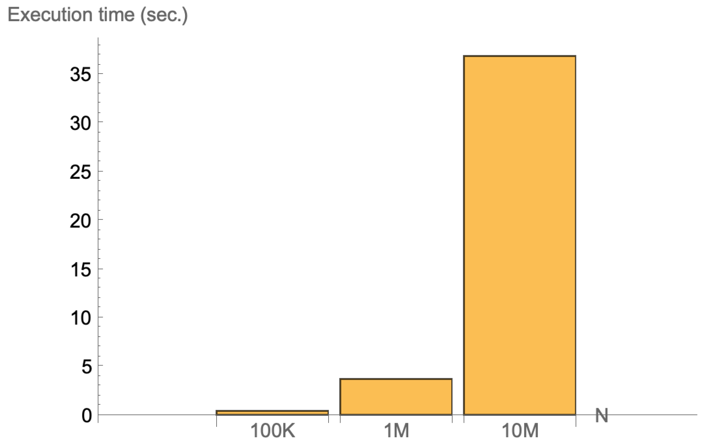
Permutation Tests Execution Time

In this subsection, we report the execution time (in seconds) for P-test using 100 K, 1 M, and 10 M random permutations. Figure 7 shows the typical execution time for the three configurations of the P-test using a MacBook Pro with 2.4 GHz Quad-Core Intel Core i5, 8 GB RAM, running Mathematica 12.3 on macOS Monterey. Figure 7 shows that we need less than half a second to perform the P-test using 100 K permutations. Less than 4 s are needed for 1 M permutations and around 37 s for 10 M permutations.

5. Conclusions and Future Work

In this paper, we advocate the use of permutation tests when comparing the performance of metaheuristic approaches. P-tests are simple and have very few assumptions about the underlying data distribution.

A test statistic was defined as the absolute difference between the medians of the samples. An algorithm is then presented for how to apply the proposed test on the results of metaheuristic methods. The proposed algorithm is implemented in Python and Wolfram Language.

The proposed P-test is compared with two classical and widely used nonparametric tests and the results show that the P-test is generally consistent with both tests. However, if there is any difference the P-test is typically more conservative than the other two tests.

We have investigated three different values for the number of permutations, N, (namely, 100,000, 1,000,000, and 10,000,000). All three values yield similar conclusions, which means that 100,000 permutations were enough for this data set.

The proposed test statistic, d, works well in most cases, except for the rare case where the standard deviation of the sample is equal to zero. In that case, the sample’s mean should be used as in Equation (3).

For future work, we will investigate using a reduced number of permutations. These permutation values are computed based on tail approximation, which is obtained by using a generalized Pareto distribution, as suggested by [25].

References

1. Yang, X.S. Nature-Inspired Optimization Algorithms; Elsevier: Amsterdam, The Netherlands, 2014. [Google Scholar]
2. Dorigo, G.D.C.M. The Ant Colony Optimization meta-heuristic. In New Ideas in Optimization; Corne, D., Dorigo, F.G.M., Eds.; McGraw Hill: London, UK, 1999; pp. 11–32. [Google Scholar]
3. Kennedy, J.; Eberhart, R. Particle Swarm Optimization. In Proceedings of the IEEE International Conference on Neural Networks, Perth, WA, Australia, 27 November–1 December 1995; pp. 1942–1948. [Google Scholar]
4. Storn, R.; Price, K. Differential Evolution—A Simple and Efficient Adaptive Scheme for Global Optimization over Continuous Spaces; Technical Report; ICSI: Berkeley, CA, USA, 1995. [Google Scholar]
5. Heidari, A.A.; Mirjalili, S.; Faris, H.; Aljarah, I.; Mafarja, M.; Chen, H. Harris hawks optimization: Algorithm and applications. Future Gener. Comput. Syst. 2019, 97, 849–872. [Google Scholar] [CrossRef]
6. Li, S.; Chen, H.; Wang, M.; Heidari, A.A.; Mirjalili, S. Slime mould algorithm: A new method for stochastic optimization. Future Gener. Comput. Syst. 2020, 111, 300–323. [Google Scholar] [CrossRef]
7. Hosseini, E.; Ghafoor, K.Z.; Emrouznejad, A.; Sadiq, A.S.; Rawat, D.B. Novel metaheuristic based on multiverse theory for optimization problems in emerging systems. Appl. Intell. 2021, 51, 3275–3292. [Google Scholar] [CrossRef] [PubMed]
8. Nabil, E. A Modified Flower Pollination Algorithm for Global Optimization. Expert Syst. Appl. 2016, 57, 192–203. [Google Scholar] [CrossRef]
9. Han, F.; Zheng, M.; Ling, Q. An improved multiobjective particle swarm optimization algorithm based on tripartite competition mechanism. Appl. Intell. 2022, 52, 5784–5816. [Google Scholar] [CrossRef]
10. Ning, Y.; Peng, Z.; Dai, Y.; Bi, D.; Wang, J. Enhanced particle swarm optimization with multi-swarm and multi-velocity for optimizing high-dimensional problems. Appl. Intell. 2019, 49, 335–351. [Google Scholar] [CrossRef]
11. Chaitanya, K.; Somayajulu, D.V.L.N.; Krishna, P.R. Memory-based approaches for eliminating premature convergence in particle swarm optimization. Appl. Intell. 2021, 51, 4575–4608. [Google Scholar] [CrossRef]
12. Tanabe, R.; Fukunaga, A. Improving the search performance of SHADE using linear population size reduction. In Proceedings of the Congress on Evolutionary Computation (CEC), Beijing, China, 6–11 June 2014; IEEE: Piscataway, NJ, USA, 2014; pp. 1658–1665. [Google Scholar]
13. Li, Y.; Wang, S.; Liu, H.; Yang, B.; Yang, H.; Zeng, M.; Wu, Z. A backtracking differential evolution with multi-mutation strategies autonomy and collaboration. Appl. Intell. 2022, 52, 3418–3444. [Google Scholar] [CrossRef]
14. Zhong, X.; Cheng, P. An elite-guided hierarchical differential evolution algorithm. Appl. Intell. 2021, 51, 4962–4983. [Google Scholar] [CrossRef]
15. Dos Santos Coelho, L.; Mariani, V.C. Use of chaotic sequences in a biologically inspired algorithm for engineering design optimization. Expert Syst. Appl. 2008, 34, 1905–1913. [Google Scholar] [CrossRef]
16. Kayhan, A.H.; Ceylan, H.; Ayvaz, M.T.; Gurarslan, G. PSOLVER: A new hybrid particle swarm optimization algorithm for solving continuous optimization problems. Expert Syst. Appl. 2010, 37, 6798–6808. [Google Scholar] [CrossRef]
17. Sörensen, K. Metaheuristics—The metaphor exposed. Int. Trans. Oper. Res. 2015, 22, 3–18. [Google Scholar] [CrossRef]
18. Camacho-Villalón, C.L.; Stützle, T.; Dorigo, M. Success-history based parameter adaptation for differential evolution. In Proceedings of the Grey Wolf, Firefly and Bat Algorithms: Three Widespread Algorithms that Do Not Contain Any Novelty, ANTS Conference 2020, Auckland, New Zealand, 29 June–4 July 2020; pp. 121–133. [Google Scholar]
19. Wilcoxon, F. Individual comparisons by ranking methods. Biom. Bull. 1945, 1, 80–83. [Google Scholar] [CrossRef]
20. LaTorre, A.; Molina, D.; Osaba, E.; Poyatos, J.; Ser, J.D.; Herrera, F. A Prescription of Methodological Guidelines for Comparing Bio-inspired Optimization Algorithms. Swarm Evol. Comput. 2021, 67, 100973. [Google Scholar] [CrossRef]
21. Derrac, J.; García, S.; Molina, D.; Herrera, F. A practical tutorial on the use of nonparametric statistical tests as a methodology for comparing evolutionary and swarm intelligence algorithms. Swarm Evol. Comput. 2011, 1, 3–18. [Google Scholar] [CrossRef]
22. Dunn, O. Multiple comparisons among means. J. Am. Can. Stat. Assoc. 1961, 56, 52–64. [Google Scholar] [CrossRef]
23. Aickin, M.; Gensler, H. Adjusting for multiple testing when reporting research results: The Bonferroni vs Holm methods. Am. J. Public Health 1996, 86, 726–728. [Google Scholar] [CrossRef] [Green Version]
24. Edgington, E. Randomization Tests; Marcel Dekker, Inc.: New York, NY, USA, 1980. [Google Scholar]
25. Knijnenburg, T.; Wessels, L.; Reinders, M.; Shmulevich, I. Fewer permutations, more accurate P-values. Bioinformatics 2009, 25, i161–i168. [Google Scholar] [CrossRef] [Green Version]
26. Skiena, S. The Data Science Design Manual; Springer: Berlin/Heidelberg, Germany, 2017. [Google Scholar]
27. Kunert-Graf, J.; Sakhanenko, N.; Galas, D. Optimized permutation testing for information theoretic measures of multi-gene interactions. BMC Bioinform. 2021, 22, 180. [Google Scholar] [CrossRef]
28. Hashim, F.A.; Houssein, E.H.; Hussain, K.; Mabrouk, M.S.; Al-Atabany, W. Honey Badger Algorithm: New metaheuristic algorithm for solving optimization problems. Math. Comput. Simul. 2022, 192, 84–110. [Google Scholar] [CrossRef]
29. Rao, R.V. Jaya: A simple and new optimization algorithm for solving constrained and unconstrained optimization problems. Int. J. Ind. Eng. Comput. 2016, 7, 19–34. [Google Scholar]
30. Chou, J.S.; Truong, D.N. A novel metaheuristic optimizer inspired by behavior of jellyfish in ocean. Appl. Math. Comput. 2021, 389, 125535. [Google Scholar] [CrossRef]
31. Tanabe, R.; Fukunaga, A. Success-history based parameter adaptation for differential evolution. In Proceedings of the Evolutionary Computation (CEC), Cancun, Mexico, 20–23 June 2013; IEEE: Piscataway, NJ, USA, 2013; pp. 71–78. [Google Scholar]
32. Yue, D.; Price, K.; P, S.; Liang, J.; Ali, M.; Qu, B.; Awad, N.; Biswas, P. Problem Definitions and Evaluation Criteria for CEC 2020 Competition on Single Objective Bound Constrained Numerical Optimization; Technical Report; Zhengzhou University: Zhengzhou, China; Nanyang Technological University: Singapore, 2019. [Google Scholar]
Figure 1. P-tests score significance by the position of d on actual data (represented as a vertical dashed line) against a distribution of statistic values generated by random permutations. (a) A position on the extreme tail shows significant difference. (b) A position within the distribution shows no significant difference.
Mathematics 10 02219 g001
Figure 2. The P-test in the Wolfram language.
Mathematics 10 02219 g002
Figure 3. Scatter plots of the competing algorithms on the 10 functions.
Mathematics 10 02219 g003
Figure 4. Box-and-Whiskers plots comparing the performance of the algorithms on the 10 functions.
Mathematics 10 02219 g004
Figure 5. The landscapes of the Expanded Schaffer (left) and HGbat (right) functions.
Mathematics 10 02219 g005
Figure 6. The distribution of statistic values from random permutations for representative functions. The dashed vertical line indicates the observed data test statistic, d.
Mathematics 10 02219 g006
Figure 7. The execution time (in seconds) of P-Test using 100,000, 1,000,000, and 10,000,000 permutations.
Mathematics 10 02219 g007