The New Second-Order Sliding Mode Control Algorithm

Abstract

A new class of regulators on the basis of the second-order sliding mode control is proposed. For the second-order system with smooth disturbances, special feedback is chosen with a discontinuous component and a radical function component. The synthesized control law provides a transient oscillatory process with decaying amplitudes, which converge to zero in finite time. In contrast to existing algorithms, the condition of homogeneity of the closed-loop system differential equations is omitted. In comparison to the “twisting”-algorithm, which is well known, designed feedback provides an invariance property with respect to smooth external perturbation with less relay amplitude. With the help of a special Lyapunov function, the convergence proof is considered by using the averaging approach. It is shown that the average oscillation period convergence speed is strictly negative, and the estimation of the convergence time is presented. The simulation results of the designed control law for the one link robot-manipulator are presented, which shows less steady-state oscillations in comparison to existing approaches.

1. Introduction

The sliding mode technique is a well-known method suitable for solving control and observation problems for systems under the influence of external perturbations and mathematical model uncertainties [1,2]. There are three main properties concerned with the sliding mode control approach:

• finite time convergence to the sliding manifold;
• full suppression of bounded external perturbations, which belong to the control space;
• reduction of the dynamical order of the system during motion along the sliding manifold.

The conventional sliding mode technique implies that the control input appears after the first differentiation of the sliding manifold [1,2]; in other words, the relative degree of the sliding manifold is equal to one. For the systems where the relative degree is greater than one, higher-order sliding mode methods have been developed, which have attracted considerable research interest in the last three decades [3,4,5,6,7,8]. In this paper, the new second-order sliding mode control law is developed. According to the definitions [5,8,9], for the second-order sliding mode, the relative degree is equal to two and the trajectories of the system converge to the intersection of the sliding manifold and its derivative in finite time. It is proposed to modify the, so called, “twisting” algorithm [5] by excluding one of the discontinuous components from the control law. This can be done with the help of the recent results in the invariance theory [10,11], with the help of the “vortex” algorithm. The proposed class of regulators is not a combination of any algorithm. We propose another paradigm. The designed control input includes continuous and discontinuous components. The discontinuous one provides nonlinear oscillations in the closed-loop system as it was done in “twisting” [12] or ”super-twisting” algorithms [13,14,15,16] and their modifications [12,17,18]. The continuous component yields the amplitudes of the oscillations to zero in finite time. The continuous term is the sum of the linear function and non-Lipschitz function [19]. In this paper, the radical function with power from zero to one is chosen as the non-Lipschitz candidate function. The continuous component has an infinite gain coefficient in origin, and this feature causes the finite time convergence property of the closed-loop system. It is necessary to note that using feedback with an arbitrary radical function has not been considered previously in the second-order sliding mode controllers, and the convergence proof for such a type of function is the challenge. From other points of view, the super-twisting algorithm supposes that the control input appears after the first differentiation of the sliding manifold. In our problem statement, the sliding surface must be twice differentiated to get the control input on the right-hand side. This is the main distinction with respect to the super-twisting algorithm and all its modifications, and it corresponds to the restriction on the class of the control plants for the super-twisting control methodology. The main advantage of the proposed controller is the reduction of the discontinuous term amplitude, which can be chosen as two times less in comparison to the ”twisting” algorithm. This is a very valuable result for adaptive [12,16] or modified [17] ”twisting” controllers, where the tuning relay bounds may be twice reduced from below.

It is necessary to note that all properties discussed above are valid only for the “ideal sliding mode”, which implies infinite switching frequency of the discontinuous control input [1]. In real practice, application designers and engineers must consider the “real sliding mode” with a finite switching frequency when the trajectories of the system belong to some small $\Delta$-vicinity of the sliding manifold. This phenomenon is called the “chattering” effect [1,7], and it is concerned with imperfections of the discontinuous functions in the real world. During “chattering”, the small amplitude oscillations appear in the output variable, which causes extra heat losses, time life reduction of the mechanical parts of the plant and low control accuracy. The steady-state oscillations amplitude strictly depends on the discontinuous control bounds, and one of the direct ways to decrease “chattering” is to reduce these. This idea is realized for the “twisting” second-order sliding mode algorithm, which is modified by the approach proposed above.

This paper is organized as follows. In Section 2, the basic definitions are introduced, and the main methods used in the paper are described. The problem statement and main idea of the synthesis of the proposed control law are presented in Section 3, and the properties of the radical function are also discussed. In Section 4, the convergence of the closed-loop system with the combined control law containing arbitrary radical function and discontinuous components is proven by qualitative analysis of the transient process and the Lyapunov function method is applied to prove the finite time reaching of the second-order sliding mode set and to get its reaching time estimation. The efficiency of the designed control laws is demonstrated in Section 5 for the one-link robot manipulator regulation. Finally, in Section 6, some concluding comments about the presented results are given and further investigation directions are discussed.

2. Basic Definitions and Methods

Consider the dynamical system

$$\dot{x}=f(t,x)$$

(1)

where $x\in R^n$ is the state space vector, t is the time, $f(t,x)={(f_1,f_2,\cdots ,f_n)}^{\mathrm{T}}$, $f(t,x)$ is the piece-wise continuous vector function in a finite domain G of an $(n+1)$-dimensional space that undergoes discontinuities on the manifold

$$s(t,x)=0,s\in R.$$

Definition 1

([20]). The solution of (1) is a continuous vector function $x\left(t\right)$ determined in the time interval I, for which the differential inclusion is fulfilled almost everywhere.

$$\dot{x}\in F(t,x),$$

(2)

where set $F(t,x)$ contains one point if $f(t,x)$ is continuous, and if $f(t,x)$ is discontinuous, the set $F(t,x)$ is given by

$$F=conv{F}_0(t,x),$$

(3)

where $F_0(t,x)$ is the set of all possible limits of $f(t,x)$ as $x^{*}\left(t\right)\notin s(x,t)=0,x^{*}\to x$, where $x^{*}$ is the continuity point of $f(t,x)$; conv means convex closure.

Definition 2

([5]). Let Γ be a smooth manifold. The set Γ itself is called the first-order sliding point set. The second-order sliding point set is defined as the set of points $x\in \Gamma$, where $F\left(x\right)$ lies in the tangential space $T_y\Gamma$ of manifold Γ at the point x.

Definition 3

([5]). It can is said that there exists the first (or the second)-order sliding mode on the manifold Γ in the vicinity of a first (or second)-order sliding point $x_0$ if, in the vicinity of the point $x_0$, the first (or second)-order sliding set is an integral set, i.e., consists of the Filippov’s sense solutions.

Consider the closed-loop control system

$$\dot{x}=f(t,x,u),$$

(4)

$$u=U(t,x,\zeta ),$$

(5)

$$\dot{\zeta }=\Psi (t,x,\zeta ),$$

(6)

where $u\in R^1$ is a control input, which may be chosen in an appropriate way, U is a feedback operator, ζ is a special auxiliary parameter. The initial value of ζ may be defined by a special function $\zeta \left(t_0\right)={\zeta }_0(t_0,x_0)$ or considered to be arbitrary.

Let $s(t,x)=0,s\in R^1$ be the desirable constraint $s\in C^1$, ${\nabla }_{x}s\ne 0$.

Definition 4

([1]). With the help of an equivalent control method, the motion of system (4) with $s(t,x)=0$ is described by the equation

$$\dot{x}=f(t,x,u_{eq}(t,x)),$$

where $u_{eq}(t,x)$ is the equivalent control that is evaluated from the equation

$$\dot{s}=s_t^{\prime }(t,x)+s_x^{\prime }(t,x)f(t,x,u_{eq}(t,x))=0,$$

(7)

where $s_t^{\prime },s_x^{\prime }$ are the corresponding derivatives.

Definition 5

([5]). Equations (5) and (6) are called the first and second-order sliding algorithms on constraint $s(x,t)=0$ if a stable sliding mode of the first (second)-order on the manifold $s(x,t)=0$ is achieved, and with every initial condition $(t_0,x_0)$ the state x is transformed to the sliding mode in finite time.

Definition 6

([5]). Let $(t,x(t,\epsilon \left)\right)$ from (4) be a family of trajectories indexed by $\epsilon \in R$ with the common initial condition $(t_0,x_0)$, and let $t\ge t_0$ (or $t\in [t_0,T]$). Assume that there exists $t_1\ge t_0$ (or $t_1\in [t_0,T]$) such that on every segment $[t^{\prime },t^{″}]$, where $t^{\prime }\ge t_1$ (or on $[t_1,T]$), the function $s(t,x(t,\epsilon \left)\right)$ tends uniformly to zero with ε tending to zero. In this case, we call such a family a real sliding family on the constraint $s(x,t)=0$. We call the motion on the interval $[t_0,t_1]$ a transient process and the motion on the interval $[t_1,\infty ]$ (or $[t_1,T]$) a steady-state process.

Definition 7

([5]). Let $\gamma \left(\epsilon \right)$ be a real-valued function such that $\gamma \left(\epsilon \right)\to 0$ as $\epsilon \to 0$. A real sliding algorithm on the constraint $s=0$ is said to be of the second-order with respect to $\gamma \left(\epsilon \right)$ if, for any compact set of initial conditions, and for any time interval $[T_1,T_2]$, there exists a constant C, such that the steady-state process satisfies

$$|s(t,x(t,\epsilon ))|\le {C|\gamma \left(\epsilon \right)|}^2$$

for $t\in [T_1,T_2]$.

Let $(t,x(t,\epsilon \left)\right)$ be a real sliding family with $\epsilon \to 0$, t belongs to a bounded interval. Let $s(t,x)$ be a smooth constraint function, and $r=2$ be the real sliding order with respect to $\tau \left(\epsilon \right)$, where $\tau \left(\epsilon \right)>0$ is the smallest time interval of smoothness of the piecewise smooth function $x(t,\epsilon )$.

Proposition 1

([5]). If the derivative $\dot{s}(t,x(t,\epsilon ))$ is uniformly bounded in ε for the steady-state part of $x(t,\epsilon )$, then there exists a positive constant $C_1$ such that for the steady-state process, the following inequality holds

$$|\dot{s}(x,t)|\le C_1\epsilon .$$

There are not so many methods for investigation of the systems with higher-order sliding modes. One of the most used approaches is to provide, if it is possible, the homogeneity property of the closed-loop system with an appropriate choice of the control input [6,21,22]. In particular, if an asymptotic convergence of the closed-loop system is proven, then for the system of homogeneous differential equations, it leads to finite time convergence. The homogeneity requirement restricts the class of systems and control algorithms that can be used during feedback design.

The classical Lyapunov functions method [23] has been extended for the systems with differential inclusions (2) in [24,25]. In [26], a non-smooth Lyapunov function is used to prove the finite-time convergence of the closed-loop system with one of the second-order sliding mode control algorithms.

The modification of V.I. Zubov’s method [27,28,29] for finding the appropriate Lyapunov function for the second-order sliding mode algorithm is proposed in [30,31,32].

The difficulties of the evaluation of a suitable Lyapunov function are slightly relaxed in [33], where an alternative approach on the basis of the combination of the Lyapunov method and the averaging approach [34] is introduced for the stability proof. This can be performed by evaluating the average decaying rate of a positive semi-definite function of the state space variables. If the upper negative bound is found for the average decaying speed, then it yields to the second-order sliding mode. This method is used in this paper for the finite time convergence proof and its estimation. The benefit of this approach is that only the upper bound of the average descending speed of some positive semi-definite function must be estimated, and only the functions for which this estimation is negative must be found. Due to this methodology, in the oscillation period, the derivative of the Lyapunov candidate function may be positive for some time interval, and in this period, only the averaged derivative must be negative. This alternative way sufficiently simplifies the search for the Lyapunov candidate function.

The methods of the classical mathematical analysis [19] are used as an auxiliary tool during each proof step.

3. Problem Statement

Consider the system

$$\begin{array}{ccc}{\dot{s}}_1\hfill & =& s_2,\hfill \\ {\dot{s}}_2\hfill & =& u+\xi \left(t\right),\hfill \end{array}$$

(8)

where $s_1,s_2\in \mathbb{R}$ are the measured state variables, $u\in \mathbb{R}$ is the control input, $|\xi (t)|<\Xi =\mathrm{const}>0$ is an unknown function of external perturbations of the system, which is assumed to be bounded and differentiable with respect to time:

$$|\dot{\xi }\left(t\right)|\le \overline{\Xi }=\mathrm{const}>0,$$

(9)

the constants $\Xi$ and $\overline{\Xi }$ are known.

The problem of the stabilization of state variables in a finite time is stated in

$$s_1\left(t\right)=s_2\left(t\right)=0,\forall t>t_r$$

(10)

by synthesis, the static feedback $u=U(s_1,s_2)$. The constant $t_r$ is not predetermined, and only its existence and evaluation are investigated.

4. Main Result

4.1. Motivation

There exists the well-known “twisting”, algorithm [3,4,5], which solves the stated problem (10). According to this feedback law, the control input is chosen in the form

$$u=-M_2\mathrm{sign}\left(s_2\right)-M_1\mathrm{sign}\left(s_1\right),$$

(11)

where $M_1=\mathrm{const}>0,M_2=\mathrm{const}>0$, $(·)$ is the sign function

$$\mathrm{sign}\left(y\right)=\left\{\begin{array}{c}1,y>0;\hfill \\ -1,y<0,\hfill \end{array}\right.$$

for $y=0$ the solutions of the closed-loop system are (8), (9) and (11) are understood in Filippov’s sense of (2) and (3), $\mathrm{sign}\left(y\right)\in [-1,1]$.

In [1,5,21,30,31], it was proven that “twisting” is a second-order sliding mode algorithm (Definition 5) under conditions

$$M_1>M_2+\Xi ,M_2>\Xi .$$

(12)

All second-order sliding mode algorithms are based on relay feedback [7,9], which provides an oscillatory character of the transient process for system variables. Adding to relay some signal that dissipates the energy, the asymptotic or finite-time convergence of controlled variables to zero can be established. In [10,11], it was shown that using the static feedback

$$u=-\alpha s_2-M\mathrm{sign}\left(s_1\right),M>\Xi ,\alpha (M-\Xi )>\overline{\Xi },$$

(13)

in (8) leads to asymptotic convergence of the variables $s_1$ and $s_2$ to the origin. The control algorithm (13) was named “vortex” due to the image of the transient process. Moreover, if the twice differentiable disturbance is included on the right-hand side of the equation for $s_1$, then the asymptotic convergence is provided for the “unmatched” perturbation (out of control space).

The nonlinear oscillator is organized by the relay component $-M\mathrm{sign}\left(s_1\right)$, and the $-\alpha s_2$ component, such as viscous friction, ensures energy dissipation in the closed-loop system. According to the stated problem, the dissipation component may be chosen in such a way to provide finite time convergence. In this paper, it is proposed to add a radical function to the feedback. It is well known [35,36,37] that the differential equation for scalar variable y with the square root function

$$\dot{y}=-\sqrt{|y|}\mathrm{sign}\left(y\right)$$

has the property of finite-time convergence. In the next subsection, a radical function will be used in the control law to provide the finite time convergence property.

4.2. Control Algorithm Choice

In this subsection, the following control input is introduced

$$\begin{array}{c}u=-\alpha s_2-\alpha {|s_2|}^{\beta }\mathrm{sign}\left(s_2\right)-M\mathrm{sign}\left(s_1\right),\beta =\mathrm{const}>0,0<\beta <1;\\ \alpha (M-\Xi )>\overline{\Xi },M>\Xi ,\alpha =\mathrm{const}>0,M=\mathrm{const}>0.\end{array}$$

(14)

Further, it will be proven that (14) is the second-order sliding mode control algorithm (Definition 5), and this result for systems (8) and (9) is achieved with two times less relay amplitude in comparison to (11).

For further considerations, the following comparison system is used

$$\begin{array}{c}{\dot{y}}_1=y_2,\hfill \\ {\dot{y}}_2=-\alpha y_2-M\mathrm{sign}\left(y_1\right)+\Xi \mathrm{sign}\left(y_2\right).\hfill \end{array}$$

(15)

The component $-M\mathrm{sign}\left(s_1\right)$ provides the oscillating behavior of the phase trajectories, and the phase portrait methods analysis is one of the main methods that can be used for convergence proof. However, for different initial conditions, the transient process for the closed-loop system can vary significantly. Further analysis will show that after one or two times switching the relay function, the state variables are involved in the oscillating character of the convergence process. In this regime, the previous results [10,11] may be used for asymptotical convergence proof. Let us clarify this idea. The following area is introduced into consideration

$$|s_2|+|s_2{|}^{\beta }\le {\displaystyle \frac{M-\Xi }{\alpha }}.$$

(16)

It is obvious that (the formula was changed from $|s_2|+|s_2{|}^{\beta }\mathrm{sign}\left(s_2\right)\ge |s_2|$)

$$|s_2|+|s_2{|}^{\beta }\ge |s_2|.$$

(17)

In this area, it was shown in [10,11] that for identical initial conditions, phase portraits of (8), (14) and (15) have the form depicted in Figure 1. It can be seen from (8), (14) and (15) that

$$\begin{array}{c}{\displaystyle \frac{\partial y_2}{\partial y_1}}={\displaystyle \frac{-\alpha y_2-M\mathrm{sign}\left(y_1\right)+\xi \left(t\right)}{y_2}},\hfill \\ {\displaystyle \frac{\partial s_2}{\partial s_1}}={\displaystyle \frac{-\alpha s_2-\alpha {|s_2|}^{\beta }\mathrm{sign}\left(s_2\right)-M\mathrm{sign}\left(s_1\right)+\xi \left(t\right)}{s_2}}.\hfill \end{array}$$

(18)

Figure 1. Phase portraits of systems (8), (14) and (15).

For example, if the third quadrant is investigated, for any points of the phase portrait $s_{2-}=y_2<0$, and the time instant t in the third quadrant is according to (14), (15) and (17)

$$\begin{array}{c}{\displaystyle \frac{\partial y_2}{\partial y_1}}={\displaystyle \frac{\alpha |s_{2-}|+M-\Xi }{s_{2-}}}<0,{\displaystyle \frac{\partial s_2}{\partial s_1}}={\displaystyle \frac{\alpha (|s_{2-}|+|s_{2-}{|}^{\beta })+M+\xi \left(t\right)}{s_{2-}}}<0;\hfill \\ {\displaystyle \frac{\left(\frac{\partial y_2}{\partial y_1}\right)}{\left(\frac{\partial s_2}{\partial s_1}\right)}}={\displaystyle \frac{\alpha |s_{2-}|+M-\Xi }{\alpha (|s_{2-}|+|s_{2-}{|}^{\beta })+M+\xi \left(t\right)}}<1.\hfill \end{array}$$

This means that curve b corresponding to the phase portrait of system (15) covers the phase portrait a of (8) and (14).

By analogy, in the second quadrant, curve b corresponding to the phase portrait of (15), covers the phase portrait a of (8) and (14), because from (16) and (18) the variable growth rate $s_2\left(t\right)$ for any point of the phase portrait $s_{2+}=y_2>0$ is less than the growth rate of the variable $y_2\left(t\right)$ (the following formula was added to the paper’s text)

$$\begin{array}{c}{\displaystyle \frac{\partial y_2}{\partial y_1}}={\displaystyle \frac{-\alpha |s_{2+}|+M+\Xi }{s_{2+}}}>0,{\displaystyle \frac{\partial s_2}{\partial s_1}}={\displaystyle \frac{-\alpha (|s_{2+}|+|s_{2+}{|}^{\beta })+M+\xi \left(t\right)}{s_{2+}}}>0;\hfill \\ {\displaystyle \frac{\left(\frac{\partial y_2}{\partial y_1}\right)}{\left(\frac{\partial s_2}{\partial s_1}\right)}}={\displaystyle \frac{-\alpha |s_{2+}|+M+\Xi }{-\alpha (|s_{2+}|+|s_{2+}{|}^{\beta })+M+\xi \left(t\right)}}>1.\hfill \end{array}$$

Of course, these arguments only are valid in space and not in time, but the phase portrait of (15) is majorant for the phase curve of (8) and (14) in the area (16). From the asymptotic stability of (15) it follows that the variables of (8) and (14) converge to zero asymptotically also

$$\underset{t\to +\infty }{lim}|s_1\left(t\right)|=0,\underset{t\to +\infty }{lim}|s_2\left(t\right)|=0.$$

Convergence to the zone (16) must be considered more carefully due to different images of the phase portrait depending on the initial conditions. For further analysis, the full transient process for (8) and (14) is separated into three main stages:

(1)

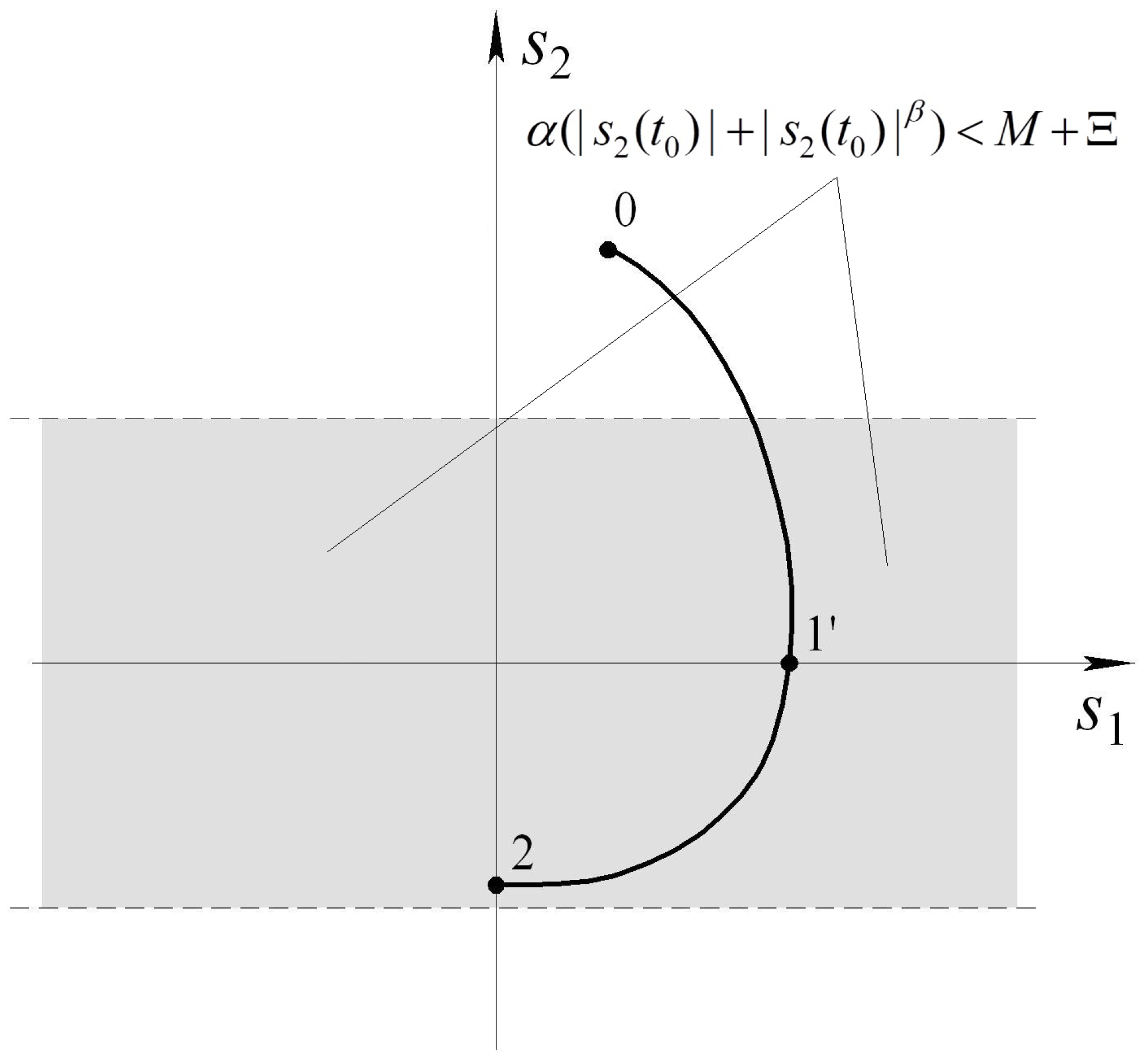
hitting the area

$$|s_2\left(t\right)|\le {\epsilon }_1={\displaystyle \frac{M+\Xi }{\alpha }};$$

(2)

convergence to the zone

$${\epsilon }_2\le |s_2\left(t\right)|\le {\displaystyle \frac{M+\Xi }{\alpha }},$$

where ${\epsilon }_2$ is some positive constant, which will be introduced below;

(3)

movement in the vicinity of the origin

$$|s_2\left(t\right)|\le {\epsilon }_2$$

to zero in finite time.

During the proof, the following notations are used, which correspond to different stages of the convergence process:

(1)

$t_0$ is the initial moment of time;

(2)

$t_1$ is the time instant at which $s_1\left(t_1\right)=0,|s_2\left(t_1\right)|+|s_2\left(t_1\right){|}^{\beta }>{\displaystyle \frac{M+\Xi }{\alpha }}$;

(3)

$t_1^{{}^{\prime }}$ is the time instant at which $s_2\left(t_1^{{}^{\prime }}\right)=0$;

(4)

$t_2$ is the time instant at which $s_1\left(t_2\right)=0,|s_2\left(t_2\right)|\le {\epsilon }_1$;

(5)

$t_3$ is the time instant at which $s_1\left(t_3\right)=0,|s_2\left(t_3\right)|\le {\epsilon }_2$;

(6)

$t_3^{{}^{\prime }}$ is the time instant at which $|s_2\left(t_3^{{}^{\prime }}\right)|\le {\epsilon }_2$, $s_1\left(t_3^{\prime }\right)=0$;

(7)

$t_r$ is the time instant of second-order sliding mode arising.

Note that depending on the initial conditions, not all of the listed stages occur in reality. Further, all possible scenarios for the events evolution will be considered in detail.

4.3. Estimation of the Time to Hit ${\epsilon }_1$-Area

Situation 1.

Consider the case with the following initial conditions (see Figure 2)

$$\alpha (|s_2\left(t_0\right)|+|s_2\left(t_0\right){|}^{\beta })>M+\Xi ,s_1\left(t_0\right)s_2\left(t_0\right)<0.$$

(19)

Figure 2. Phase portraits under initial conditions from the second and fourth quadrants (Situation 1).

This situation corresponds to the case when the initial point of the phase portrait is in the second and the fourth quadrants of the phase plane. Let us show that the greater the decreasing rate of the variable $s_2\left(t\right)$, then the larger the estimation of the time interval $t_1-t_0$ (stages 1–2). For this, we consider the system

$$\begin{array}{c}{\dot{s}}_1^{*}=s_2^{*},\hfill \\ {\dot{s}}_2^{*}=-v\mathrm{sign}\left(s_1^{*}\right),\hfill \\ s_1^{*}\left(t_0\right)=s_1\left(t_0\right),s_2^{*}\left(t_0\right)=s_2\left(t_0\right),v=\mathrm{const}>0\hfill \end{array}$$

and introduce some value $s_1^{\prime }=\mathrm{const}>0,0<s_1^{\prime }<|s_1\left(t_0\right)|$.

After integration, the solution of this system is

$$\left\{\begin{array}{c}|s_2^{*}\left(t\right)|=|s_2^{*}\left(t_0\right)|-v(t-t_0),\hfill \\ |s_1^{*}\left(t\right)|=|s_1^{*}\left(t_0\right)|-|s_2^{*}\left(t_0\right)|(t-t_0)\mathrm{sign}\left(s_1^{*}\right)+{\displaystyle \frac{{(t-t_0)}^2}{2}}v\mathrm{sign}\left(s_1^{*}\right),\hfill \end{array}\right.t\ge t_0$$

and the estimation of the time interval $t_0^{\prime }-t_0$ ($t_0^{\prime }$ corresponds $|s_1^{*}\left(t_0^{\prime }\right)|=s_1^{\prime }$) can be computed from the second equality of this system by solving quadratic equation:

$$t_0^{\prime }-t_0\le {\displaystyle \frac{2(|s_1\left(t_0\right)|-s_1^{\prime })}{|s_2\left(t_0\right)|+\sqrt{s_2^2\left(t_0\right)-2v(|s_1\left(t_0\right)|-s_1^{\prime })}}}.$$

(20)

It can be seen from the last estimation that the larger value of v leads to a longer transient time. This expression has sense if the radical expression is positive. Two variants must be considered.

The first one corresponds to the phase portrait a in Figure 2, and for the maximum transient time we choose $s_1^{\prime }=0\Rightarrow t_0^{\prime }=t_1$. In this case, the initial conditions are

$$s_2^2\left(t_0\right)-2v_{\max }|s_1\left(t_0\right)|\ge 0,v_{\max }=\alpha (|s_2\left(t_0\right)|+|s_2\left(t_0\right){|}^{\beta })-M+\Xi ,$$

(21)

and for (8) and (14) with the help of (20) the following inequality is valid

$${\Delta }_1=t_1-t_0\le {\displaystyle \frac{2|s_1\left(t_0\right)|}{|s_2\left(t_0\right)|+\sqrt{s_2^2\left(t_0\right)-2v_{\max }|s_1\left(t_0\right)|}}},$$

(22)

the value $v_{\max }$ is chosen to get the maximum possible bound for the time interval estimation, because under condition (19) according to (8) and (14)

$$|{\dot{s}}_2|\le v_{\max }.$$

For the second variant (the phase portrait b in Figure 2), the initial conditions correspond to

$$s_2^2\left(t_0\right)-2v_{\max }|s_1\left(t_0\right)|<0,$$

(23)

and the estimation of the time interval $t_1-t_0$ with the help of (22) is not possible.

The part ${00}^{″}1$ of the curve b (see Figure 2) corresponds to the majorant of the phase portrait of (8) and (14) (it lies below the real curve), and $s_{2\min }$ is computed according to

$$\alpha (|s_{2\min }|+|s_{2\min }{|}^{\beta })=M-\Xi .$$

(24)

The value of $s_{\min }$ can be found by using numerical methods. $s_{\min }$ is the minimal possible speed of the variable $s_1\left(t\right)$ growth under conditions (19) and (23), and the interval $t_1-t_0$ estimation under (23) is

$${\Delta }_1=t_1-t_0\le {\displaystyle \frac{|s_1\left(t_0\right)|}{s_{2\min }}},s_2^2\left(t_0\right)-2v_{\max }|s_1\left(t_0\right)|<0.$$

(25)

Further, the time interval $t_2-t_1$ is investigated (stages 2–4).

It was mentioned earlier that the time of motion in the first and third quadrants for (8) and (14) is less than for (15) (for the parts ${11}^{\prime }$ of the curves $a,b$ see Figure 2). Taking into account that $|s_2\left(t_1\right)|\le |s_2\left(t_0\right)|$, one can write the interval estimation $t_1^{\prime }-t_1$ from (15) (see also [11])

$$\begin{array}{c}{t}_1^{\prime }-t_1\le {\displaystyle \frac{1}{\alpha }}\ln \left({\displaystyle \frac{\alpha |s_2\left(t_0\right)|+M-\Xi }{M-\Xi }}\right),\\ |s_1\left(t_1^{\prime }\right)|\le \left|-{\displaystyle \frac{M-\Xi }{{\alpha }^2}}\ln \left({\displaystyle \frac{\alpha |s_2\left(t_0\right)|+M-\Xi }{M-\Xi }}\right)+{\displaystyle \frac{|s_2\left(t_0\right)|}{\alpha }}\right|.\end{array}$$

(26)

In order to formalize the growth rate of $|s_2\left(t\right)|$ in the interval $t_2-t_1^{\prime }$ (stages 3–4, see Figure 2), the following comparison system is considered (${\tilde{s}}_2\left(t_1^{\prime }\right)=s_2\left(t_1^{\prime }\right)=0$)

$$\begin{array}{c}{\dot{\tilde{s}}}_2=-\alpha {\tilde{s}}_2+\alpha {|s_{2\min }|}^{\beta }-(M-\Xi )\mathrm{sign}\left(s_1\right),\\ |s_2\left(t\right)|\ge |{\tilde{s}}_2\left(t\right)|=\left[{\displaystyle \frac{M-\Xi }{\alpha }}-{|s_{2\min }|}^{\beta }\right]\left(1-e^{-\alpha (t-t_1^{\prime })}\right),t\ge t_1^{\prime },\end{array}$$

(27)

where $s_{2\min }$ is from (24).

The interval $t_2-t_1^{\prime }$ can be separated by two subintervals $[t_1^{*}-t_1^{{}^{\prime }}],[t_2-t_1^{*}]$. In the first subinterval $[t_1^{*}-t_1^{{}^{\prime }}]$$|s_2\left(t\right)|$ is bounded from below according to (27), and the the minimum transient time for the worst case is computed with the help of (8) and (14)

$$\begin{array}{c}|{\dot{s}}_2\left(t\right)|\le M-\Xi ,t_2-t_1^{\prime }\ge \sqrt{{\displaystyle \frac{2|s_1\left(t_1^{\prime }\right)|}{M-\Xi }}}.\end{array}$$

Therefore, one can chose the estimation of the first subinterval and the value of $|s_2\left(t_1^{*}\right)|$ concerned with it

$$t_1^{*}-t_1^{\prime }=\sqrt{{\displaystyle \frac{2|s_1\left(t_1^{\prime }\right)|}{M-\Xi }}},|s_2\left(t_1^{*}\right)|\ge \left[{\displaystyle \frac{M-\Xi }{\alpha }}-{|s_{2\min }|}^{\beta }\right]\left(1-e^{-\alpha \sqrt{\frac{2|s_1\left(t_1^{\prime }\right)|}{M-\Xi }}}\right).$$

(28)

In the second subinterval $[t_2-t_1^{*}]$ (see Figure 2)

$$\begin{array}{c}|{\dot{s}}_1\left(t\right)|\ge |s_2\left(t_1^{*}\right)|,t_2-t_1^{*}\le {\displaystyle \frac{|s_1\left(t_1^{\prime }\right)|}{|s_2\left(t_1^{*}\right)|}}.\end{array}$$

(29)

Combining (28) and (29), the following estimation can be written

$$\begin{array}{c}{t}_2-t_1^{\prime }\le \sqrt{{\displaystyle \frac{2|s_1\left(t_1^{\prime }\right)|}{M-\Xi }}}+{\displaystyle \frac{|s_1\left(t_1^{\prime }\right)|}{\left[{\displaystyle \frac{M-\Xi }{\alpha }}-{|s_{2\min }|}^{\beta }\right]\left(1-e^{-\alpha \sqrt{\frac{2|s_1\left(t_1^{\prime }\right)|}{M-\Xi }}}\right)}}.\end{array}$$

(30)

For the second time interval, one can write the inequality taking into account (26) and (30)

$$\begin{array}{c}{\Delta }_2=t_2-t_1\le {\displaystyle \frac{1}{\alpha }}\ln \left({\displaystyle \frac{\alpha |s_2\left(t_0\right)|+M-\Xi }{M-\Xi }}\right)+\sqrt{{\displaystyle \frac{2|s_1\left(t_1^{\prime }\right)|}{M-\Xi }}}+\hfill \\ +{\displaystyle \frac{|s_1\left(t_1^{\prime }\right)|}{\left[{\displaystyle \frac{M-\Xi }{\alpha }}-{|s_{2\min }|}^{\beta }\right]\left(1-e^{-\alpha \sqrt{\frac{2|s_1\left(t_1^{\prime }\right)|}{M-\Xi }}}\right)}};\hfill \\ |s_1\left(t_1^{\prime }\right)|\le \left|-{\displaystyle \frac{M-\Xi }{{\alpha }^2}}\ln \left({\displaystyle \frac{\alpha |s_2\left(t_0\right)|+M-\Xi }{M-\Xi }}\right)+{\displaystyle \frac{|s_2\left(t_0\right)|}{\alpha }}\right|.\hfill \end{array}$$

(31)

Situation 2.

Similar reasoning can be given for the case$s_1\left(t_0\right)s_2\left(t_0\right)>0$(see Figure 3). In this scenario, according to (26), the estimate of the time interval$t_1^{\prime }-t_0$is

$$\begin{array}{c}{t}_1^{\prime }-t_0\le {\displaystyle \frac{1}{\alpha }}\ln \left({\displaystyle \frac{\alpha |s_2\left(t_0\right)|+M-\Xi }{M-\Xi }}\right),\\ |s_1\left(t_1^{\prime }\right)|\le |s_1\left(t_0\right)|+\left|-{\displaystyle \frac{M-\Xi }{{\alpha }^2}}\ln \left({\displaystyle \frac{\alpha |s_2\left(t_0\right)|+M-\Xi }{M-\Xi }}\right)+{\displaystyle \frac{|s_2\left(t_0\right)|}{\alpha }}\right|.\end{array}$$

(32)

and the full time interval$t_2-t_0$can be written from inequalities (30) and (32)

$$\begin{array}{c}{\Delta }_2=t_2-t_0\le {\displaystyle \frac{1}{\alpha }}\ln \left({\displaystyle \frac{\alpha |s_2\left(t_0\right)|+M-\Xi }{M-\Xi }}\right)+\sqrt{{\displaystyle \frac{2|s_1\left(t_1^{\prime }\right)|}{M-\Xi }}}+\\ +{\displaystyle \frac{|s_1\left(t_1^{\prime }\right)|}{\left[{\displaystyle \frac{M-\Xi }{\alpha }}-{|s_{2\min }|}^{\beta }\right]\left(1-e^{-\alpha \sqrt{\frac{2|s_1\left(t_1^{\prime }\right)|}{M-\Xi }}}\right)}};\\ |s_1\left(t_1^{\prime }\right)|\le |s_1\left(t_0\right)|+\left|-{\displaystyle \frac{M-\Xi }{{\alpha }^2}}\ln \left({\displaystyle \frac{\alpha |s_2\left(t_0\right)|+M-\Xi }{M-\Xi }}\right)+{\displaystyle \frac{|s_2\left(t_0\right)|}{\alpha }}\right|.\end{array}$$

(33)

Figure 3. Phase portraits under initial conditions from the first and third quadrants (Situation 2).

4.4. Special Case of Motion in ${\epsilon }_1$-Area

Situation 3.

The initial conditions are (see Figure 4)

$$\alpha (|s_2\left(t_0\right)+|s_2\left(t_0\right){|}^{\beta })<M+\Xi ,s_1\left(t_0\right)s_2\left(t_0\right)<0.$$

Figure 4. Phase portraits under initial conditions from the second and fourth quadrants (Situation 3).

Two scenarios are considered for this situation.

The first one corresponds to the following initial conditions (phase portraits a and b in Figure 4, stage 2–3 is absent)

$$\left\{\begin{array}{c}\alpha (|s_2\left(t_0\right)+|s_2\left(t_0\right){|}^{\beta })>M-\Xi ,\hfill \\ {\Delta }_2=t_2-t_0\le {\displaystyle \frac{2|s_1\left(t_0\right)|}{|s_2\left(t_0\right)|+\sqrt{s_2^2\left(t_0\right)-2v_{\max }|s_1\left(t_0\right)|}}}),s_2^2\left(t_0\right)-2v_{\max }|s_1\left(t_0\right)|\ge 0;\hfill \\ {\Delta }_2=t_2-t_0\le {\displaystyle \frac{|s_1\left(t_0\right)|}{s_{2\min }}},s_2^2\left(t_0\right)-2v_{\max }|s_1\left(t_0\right)|<0.\hfill \end{array}\right.$$

(34)

Let us consider in more detail the case when the initial conditions for $s_2\left(t\right)$ are $\alpha (|s_2\left(t_0\right)+|s_2\left(t_0\right){|}^{\beta })<M-\Xi$ (see the c phase portrait in Figure 4). Like it was previously done in (27), the value of $|s_2\left(t\right)|$ is bounded from below by function ${\tilde{s}}_2\left(t\right)$

$$\begin{array}{c}{\dot{\tilde{s}}}_2=-\alpha {\tilde{s}}_2+\alpha |s_{2\min }{|}^{\beta }-(M-\Xi )\mathrm{sign}\left(s_1\right),|{\tilde{s}}_2\left(t_0\right)|=|s_2\left(t_0\right)|,\\ |s_2\left(t\right)|\ge |{\tilde{s}}_2\left(t\right)|=|s_2\left(t_0\right)|e^{-\alpha (t-t_0)}+\left[{\displaystyle \frac{M-\Xi }{\alpha }}-{|s_{2\min }|}^{\beta }\right]\left(1-e^{-\alpha (t-t_0)}\right),t_0\le t\le t_2.\end{array}$$

(35)

For the minimal transient time

$$t_1^{*}-t_0=\sqrt{{\displaystyle \frac{2|s_1\left(t_0\right)|}{M-\Xi }}},$$

the value $|s_2\left(t_1^{*}\right)|$ is

$$|s_2\left(t_1^{*}\right)|\ge |s_2\left(t_0\right)|e^{-\alpha \sqrt{\frac{2|s_1\left(t_0\right)|}{M-\Xi }}}+\left[{\displaystyle \frac{M-\Xi }{\alpha }}-{|s_{2\min }|}^{\beta }\right]\left(1-e^{-\alpha \sqrt{\frac{2|s_1\left(t_0\right)|}{M-\Xi }}}\right).$$

Therefore, the time interval $t_2-t_0$ is bounded by

$$\begin{array}{c}{\Delta }_2=t_2-t_0\le {\displaystyle \frac{|s_1\left(t_0\right)|}{|s_2\left(t_0\right)|e^{-\alpha \sqrt{\frac{2|s_1\left(t_0\right)|}{M-\Xi }}}+\left[\frac{M-\Xi }{\alpha }-{|s_{2\min }|}^{\beta }\right]\left(1-e^{-\alpha \sqrt{\frac{2|s_1\left(t_0\right)|}{M-\Xi }}}\right)}}+\hfill \\ +\sqrt{{\displaystyle \frac{2|s_1\left(t_0\right)|}{M-\Xi }}}.\hfill \end{array}$$

(36)

4.5. Estimated Time to Hit ${\epsilon }_2$-Area

It was shown in [10] that for $y_2\left(t\right)$ from (15) in the ${\epsilon }_1$-domain ($t\ge t_2$) there is an exponential majorant

$$|y_2\left(t\right)|\le {\displaystyle \frac{M+\Xi }{\alpha }}{e}^{-\frac{{\gamma }_0}{2}(t-t_2)},t\ge t_2,$$

(37)

where

$$\begin{array}{c}{\gamma }_0={\displaystyle \frac{\alpha (M-\Xi )}{2(M+\Xi )}}\ln \left({\displaystyle \frac{1}{1-0.533c}}\right),c={\displaystyle \frac{M-\Xi -\frac{\overline{\Xi }}{\alpha }}{M+\Xi }}.\hfill \end{array}$$

Using this inequality, the majorant for $s_2\left(t\right)$ can be written, and the estimation of the time reaching from ${\epsilon }_1$-area into some ${\epsilon }_2$-domain can be computed. To do this, the time instants are introduced $t_{2s}>t_2,t_{2y}>t_2$

$$s_1\left(t_{2s}\right)=0,y_1\left(t_{2y}\right)=0.$$

It was discussed above that $|s_2\left(t_{2s}\right)|\le |y_2\left(t_{2y}\right)|$. Inequality (37) was obtained for the following time interval estimates [11]:

$$t_{2y}-t_2\le {\displaystyle \frac{2{\epsilon }_1}{M-\Xi }}.$$

Let us find an estimate of the time interval $t_{2s}-t_2$ for (8) and (14) and, by entering a correction factor, write the resulting majorant for $s_2\left(t\right)$. Denote $t_2^{\prime }(t_2^{\prime }>t_2)$ as the nearest point in time at which $s_2\left(t_2^{\prime }\right)=0$. Then, the estimation of the time interval $t_2^{{}^{\prime }}-t_2$ and value $|s_1\left(t_2^{\prime }\right)|$ computed from (8) and (14) are

$$\begin{array}{c}|{\dot{s}}_2\left(t\right)|\ge M-\Xi ,t_2^{{}^{\prime }}-t_2={\displaystyle \frac{{\epsilon }_1}{M-\Xi }},|s_1\left(t_2^{\prime }\right)|\le {\displaystyle \frac{{\epsilon }_1^2}{2(M-\Xi )}}.\end{array}$$

(38)

The bound for the interval $t_{2s}-t_2^{{}^{\prime }}$ can be calculated from (30) by substitution estimation $|s_1\left(t_2^{\prime }\right)|$ instead of $|s_1\left(t_1^{\prime }\right)|$

$$\begin{array}{c}{t}_{2s}-t_2^{\prime }\le {\displaystyle \frac{{\epsilon }_1}{M-\Xi }}+{\displaystyle \frac{{\epsilon }_1^2}{2(M-\Xi )\left[{\displaystyle \frac{M-\Xi }{\alpha }}-{|s_{2\min }|}^{\beta }\right]\left(1-e^{-\alpha \frac{{\epsilon }_1}{M-\Xi }}\right)}}.\end{array}$$

(39)

Combining (38) and (39), one can get

$$t_{2s}-t_2\le c\left({\epsilon }_1\right){\displaystyle \frac{{\epsilon }_1}{M-\Xi }},$$

(40)

where $c\left({\epsilon }_1\right)$ is

$$c\left({\epsilon }_1\right)=\left(2+{\displaystyle \frac{{\epsilon }_1}{2\left[{\displaystyle \frac{M-\Xi }{\alpha }}-{|s_{2\min }|}^{\beta }\right]\left(1-e^{-\alpha \frac{{\epsilon }_1}{M-\Xi }}\right)}}\right).$$

According to (37) and (40) and inequality $|s_2\left(t_{2s}\right)|\le |y_2\left(t_{2y}\right)|$, the majorant for $|s_2\left(t\right)|$, $t\ge t_2$ is

$$\begin{array}{c}|s_2\left(t\right)|\le {\epsilon }_1{e}^{\gamma (t-t_2)},\gamma ={\displaystyle \frac{\alpha (M-\Xi )}{2c\left({\epsilon }_1\right)(M+\Xi )}}\ln \left({\displaystyle \frac{1}{1-0.533c}}\right).\end{array}$$

(41)

Then, the following estimation is valid for the time interval of reaching $|s_2\left(t\right)|$ from the ${\epsilon }_1$-region in some ${\epsilon }_2$-neighborhood

$${\Delta }_3=t_3-t_2\le {\displaystyle \frac{1}{\gamma }}\ln {\displaystyle \frac{{\epsilon }_1}{{\epsilon }_2}}.$$

(42)

The size of the ${\epsilon }_2$-area will be chosen in the next subsection.

4.6. Estimation of Motion Time in ${\epsilon }_2$-Domain

To estimate the time of motion at the last stage, consider the Lyapunov candidate function

$$V={\left(|s_1|-{\displaystyle \frac{\xi }{M}}{s}_1+{\displaystyle \frac{{(\alpha s_1+s_2)}^2}{2M}}\right)}^{\frac{1-\beta }{2}},$$

(43)

whose derivative along the trajectories of the system (8) and (14) has the form

$$\dot{V}\le {\displaystyle \frac{-\overline{\alpha }|s_1|-{\displaystyle \frac{{\alpha }^2}{M}}|s_2{|}^{\beta }{s}_1\mathrm{sign}\left(s_2\right)-{\displaystyle \frac{\alpha }{M}}{|s_2|}^{1+\beta }}{{\left(|s_1|-{\displaystyle \frac{\xi }{M}}{s}_1+{\displaystyle \frac{{(\alpha s_1+s_2)}^2}{2M}}\right)}^{\frac{1+\beta }{2}}}},$$

(44)

where $\overline{\alpha }=\alpha \left(1-{\displaystyle \frac{\Xi }{M}}\right)-{\displaystyle \frac{\overline{\Xi }}{M}}$. The trajectories of (8) and (14) are investigated on a half-cycle of oscillation under the initial conditions

$$s_1\left(t_3\right)=0,s_2\left(t_3\right)=-{\epsilon }_2.$$

(45)

The sign of the variable $s_2\left(t\right)$ is chosen for determinacy. In this case, on the phase plane, the system motions occur in the third and the second quadrants. Let us introduce time instant $t_4>t_3$ such that

$$s_1\left(t_4\right)=0.$$

Let us show that for a certain choice of parameters of (14) and size of ${\epsilon }_2$-domains, the derivative of the Lyapunov function (44) is not positive. For this, the fraction numerator of (44) is considered

$$z=-\overline{\alpha }|s_1|-{\displaystyle \frac{{\alpha }^2}{M}}|s_2{|}^{\beta }{s}_1\mathrm{sign}\left(s_2\right)-{\displaystyle \frac{\alpha }{M}}{|s_2|}^{1+\beta }.$$

(46)

Its partial derivatives with respect to $s_1$ and $s_2$ are

$$\begin{array}{c}{\displaystyle \frac{\partial z}{\partial s_1}}=-\overline{\alpha }\mathrm{sign}\left(s_1\right)-{\displaystyle \frac{{\alpha }^2}{M}}{|s_2|}^{\beta }\mathrm{sign}\left(s_2\right),\hfill \\ {\displaystyle \frac{\partial z}{\partial s_2}}=-{\displaystyle \frac{{\alpha }^2\beta s_1{|s_2|}^{\beta -1}}{M}}-{\displaystyle \frac{\alpha (1+\beta )}{M}}{|s_2|}^{\beta }.\hfill \end{array}$$

(47)

Let us study function z in the domain bounded by the straight lines

$$s_1=-c_s=\mathrm{const}<0,s_1=0,s_2=0,s_2={\epsilon }_2.$$

It is well known [19] that the smallest and the largest value of a function of two variables can be found from its local extremum points and from the study of the function at the boundaries of the region and in the “corner points”.

It is seen on the boundaries $s_1=0$ and $s_2=0$ and in the third quadrant ($s_1<0s_2<0$) the z is negative.

The behavior of z on the boundary $s_1=-c_s$ is studied using the second partial derivative from (47), and there is a maximum point on the level line $s_1=-c_s$ at

$$s_2={\displaystyle \frac{\alpha c_s\beta }{\beta +1}}.$$

The substitution of the obtained extremum value into (46) leads to

$$\begin{array}{c}z=-c_s\left(\overline{\alpha }-{\displaystyle \frac{{\alpha }^2}{M}}{\displaystyle \frac{|s_2{|}^{\beta }}{(\beta +1)}}\right).\hfill \end{array}$$

Taking into account the exponential convergence in the ${\epsilon }_1$-region, we introduce the size of the ${\epsilon }_2$-region, in which z is negative on the level lines $s_1=-c_s$

$${\epsilon }_2={\left({\displaystyle \frac{\overline{\alpha }M(\beta +1)}{{\alpha }^2}}\right)}^{\frac{1}{\beta }}.$$

(48)

On the other hand, in the second quadrant on the bound $s_2={\epsilon }_2$, the function z is negative under condition

$$z\le -|s_1|(\overline{\alpha }-{\displaystyle \frac{{\alpha }^2}{M}}{\epsilon }_2^{\beta })\le 0,\forall {\epsilon }_2\le {\left({\displaystyle \frac{\overline{\alpha }M}{{\alpha }^2}}\right)}^{\frac{1}{\beta }}.$$

(49)

Thereforee, comparing (48) and (49), the value of ${\epsilon }_2$ is chosen according to (49).

Now z is investigated for the local extrema. By equaling the partial derivatives (47) to zero, the suspicious points for extremums can be found

$$s_1=-{\displaystyle \frac{1+\beta }{\alpha \beta }}{\left({\displaystyle \frac{\overline{\alpha }M}{{\alpha }^2}}\right)}^{\frac{1}{\beta }},s_2={\left({\displaystyle \frac{\overline{\alpha }M}{{\alpha }^2}}\right)}^{\frac{1}{\beta }}.$$

The test of sufficient conditions

$$\begin{array}{c}{\displaystyle \frac{{\partial }^{2}z}{\partial s_1^2}}=0,{\displaystyle \frac{{\partial }^{2}z}{\partial s_1\partial s_2}}=-{\displaystyle \frac{{\alpha }^2\beta {|s_2|}^{\beta -1}}{M}};\\ {\displaystyle \frac{{\partial }^{2}z}{\partial s_2^2}}=-{\displaystyle \frac{(\beta -1){\alpha }^2\beta s_1{|s_2|}^{\beta -2}}{M}}-{\displaystyle \frac{\alpha \beta (1+\beta )}{M}}{|s_2|}^{\beta -1};\\ \left|\begin{array}{cc}{\displaystyle \frac{{\partial }^{2}z}{\partial s_1^2}}& {\displaystyle \frac{{\partial }^{2}z}{\partial s_1\partial s_2}}\\ {\displaystyle \frac{{\partial }^{2}z}{\partial s_1\partial s_2}}& {\displaystyle \frac{{\partial }^{2}z}{\partial s_1\partial s_2}}\end{array}\right|=-{\left({\displaystyle \frac{{\partial }^{2}z}{\partial s_1\partial s_2}}\right)}^2<0,\end{array}$$

shows that this is the saddle point.

Finally, the choice of the ${\epsilon }_2$-area size according to (49) guarantees that the derivative of the Lyapunov function (44) is negative in the second and third quadrants.

The asymptotic convergence of the variables of the system (8) and (14) to zero implies the inequality

$$|s_2\left(t_4\right)|<|s_2\left(t_3\right)|={\epsilon }_2,$$

using which the upper bound for (44) can be rewritten in the third quadrant ($s_1<0,s_2<0$):

$$\begin{array}{c}\dot{V}\le -{\left(2M\right)}^{\frac{1+\beta }{2}}{\displaystyle \frac{\overline{\alpha }|s_1|+{\displaystyle \frac{{\alpha }^2}{M}}|s_2{|}^{\beta }{s}_1\mathrm{sign}\left(s_2\right)+{\displaystyle \frac{\alpha }{M}}{|s_2|}^{1+\beta }}{{{\epsilon }_2}^{1+\beta }}}\le -2^{\frac{\beta }{2}}\sqrt{2}\alpha M^{\frac{\beta -1}{2}}{\displaystyle \frac{|s_2{|}^{1+\beta }}{{{\epsilon }_2}^{1+\beta }}}.\end{array}$$

(50)

The time interval $t_4-t_3$ is estimated like in (40)

$$t_4-t_3\le \left(2+{\displaystyle \frac{{\epsilon }_2}{2\left[{\displaystyle \frac{M-\Xi }{\alpha }}-{|s_{2\min }|}^{\beta }\right]\left(1-e^{-\alpha \frac{{\epsilon }_2}{M-\Xi }}\right)}}\right){\displaystyle \frac{{\epsilon }_2}{M-\Xi }}.$$

(51)

The average value of (50) is in the time interval $t\in \left[t_3,t_4\right]$, taking into account that for the second quadrant $\dot{V}\le 0$ ($t_3^{\prime }\le t\le t_4$)

$${\dot{V}}_{av}={\displaystyle \frac{1}{t_4-t_3}}\underset{t_3}{\overset{t_4}{\int }}\dot{V}\le -{\displaystyle \frac{2^{\frac{\beta }{2}}\sqrt{2}\alpha M^{\frac{\beta -1}{2}}}{{\epsilon }_2^{1+\beta }(t_4-t_3)}}\underset{t_3}{\overset{t_3^{\prime }}{\int }}{|s_2\left(\tau \right)|}^{1+\beta }d\tau .$$

(52)

In the third quadrant, the inequalities are valid

$$\begin{array}{c}{\dot{s}}_2\le v,s_2\left(t\right)\le -{\epsilon }_2+v(t-t_3),t_3\le t\le t_{3r};\\ v=\alpha ({\epsilon }_2+{\epsilon }_2^{\beta })+M+\Xi \le 2(M+\Xi ),t_{3r}-t_3={\displaystyle \frac{{\epsilon }_2}{v}}.\end{array}$$

This majorant is chosen to get the minimal value of the integral from the right-hand side of (52)

$$\underset{t_3}{\overset{t_3^{\prime }}{\int }}|s_2{\left(\tau \right)|}^{1+\beta }d\tau \ge \underset{t_3}{\overset{t_{3r}}{\int }}{|-{\epsilon }_2+v(\tau -t_3)|}^{1+\beta }d\tau \le {\displaystyle \frac{{\epsilon }_2^{2+\beta }}{2(2+\beta )(M+\Xi )}}.$$

(53)

The substitution of (51) and (53) into (52) leads to

$${\dot{V}}_{av}\le -{\displaystyle \frac{2^{\frac{\beta }{2}}\alpha M^{\frac{\beta -1}{2}}(M-\Xi )}{\sqrt{2}(2+\beta )(M+\Xi )\left(2+\frac{{\epsilon }_2}{2\left[\frac{M-\Xi }{\alpha }-{|s_{2\min }|}^{\beta }\right]\left(1-e^{-\alpha \frac{{\epsilon }_2}{M-\Xi }}\right)}\right)}}.$$

(54)

The upper bound of the convergence time to zero inside the ${\epsilon }_2$-zone is computed according to

$${\Delta }_4=t_r-t_3\le {\displaystyle \frac{V\left(t_3\right)}{|{\dot{V}}_{av}|}}={\displaystyle \frac{(2+\beta )(M+\Xi )\left(2+{\displaystyle \frac{{\epsilon }_2}{2\left[\frac{M-\Xi }{\alpha }-{|s_{2\min }|}^{\beta }\right]\left(1-e^{-\alpha \frac{{\epsilon }_2}{M-\Xi }}\right)}}\right){\epsilon }_2^{1-\beta }}{\alpha (M-\Xi )}}.$$

(55)

The upper bound for the full convergence time $t_r-t_0$ is calculated with the help of (22), (25), (31), (33), (34), (36), (42) and (55), and it is equal to ${\displaystyle \sum _{i=1}^4}{\Delta }_i$ for Situation 1 and ${\displaystyle \sum _{i=2}^4}{\Delta }_i$ for the other situations.

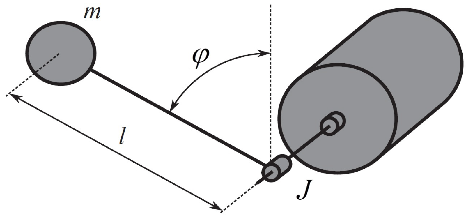
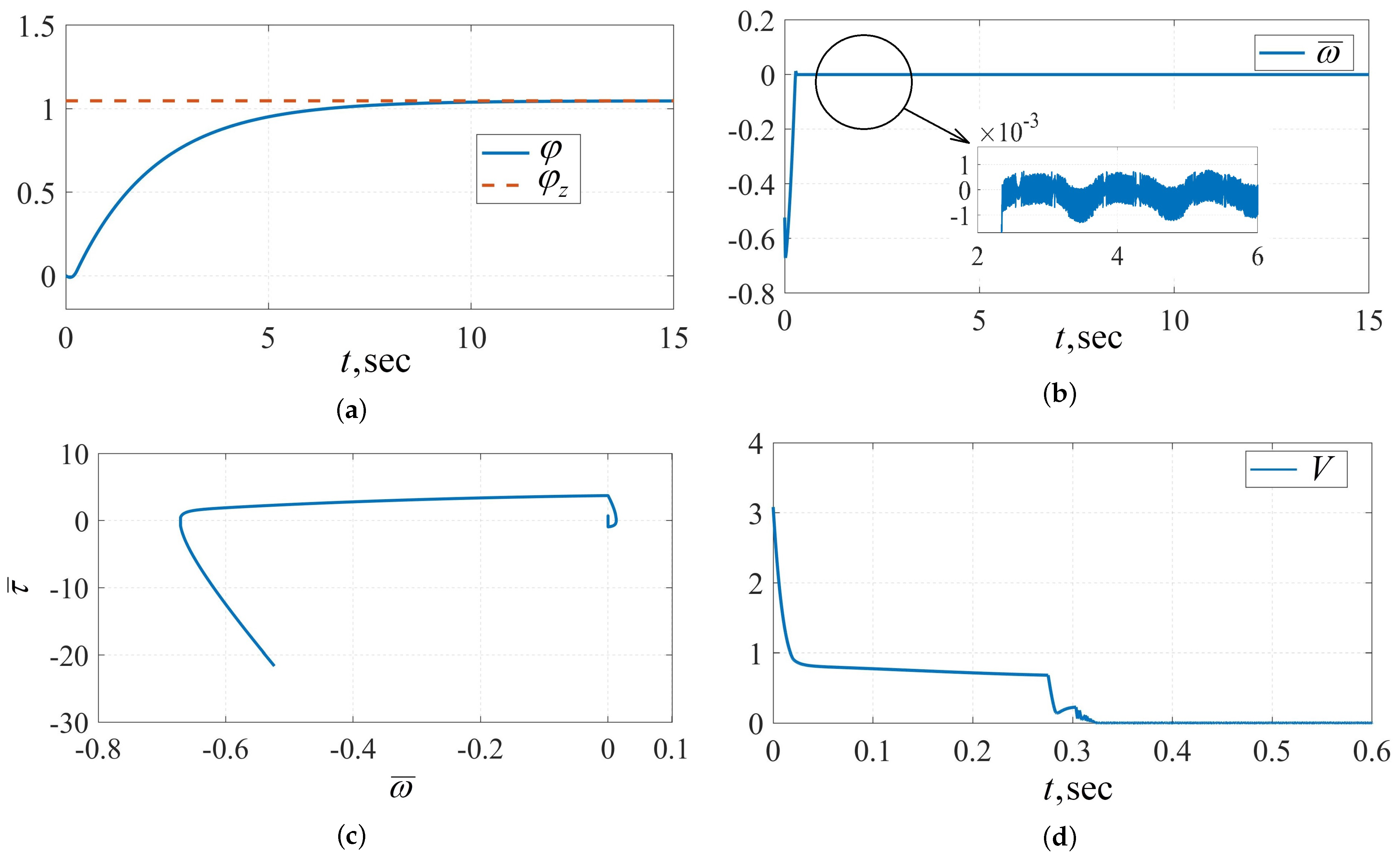
5. Numerical Example

For the numerical example, a one-link robot manipulator with a dynamical actuator is considered (see Figure 5).

$$\begin{array}{c}\dot{\phi }=\omega ,\hfill \\ \dot{\omega }={\displaystyle \frac{1}{J}}\left(\tau -mglcos\phi \right),\hfill \\ \dot{\tau }=-k\tau +u+\xi \left(t\right),\hfill \end{array}$$

(56)

where $\phi$ is the angular position of the robot arm, $\left[\mathrm{rad}\right]$; $\omega$ is the angular velocity, $[\mathrm{rad}/\mathrm{s}]$; $\tau$ is the actuator torque, $[\mathrm{N}·\mathrm{m}]$; u is the control input, $\left[\right(\Omega ·\mathrm{N}·\mathrm{m})/\mathrm{H}]$; J is the generalized inertia, $[\mathrm{kg}·{\mathrm{m}}^2]$; m is the mass of the arm of the robot, $\left[\mathrm{kg}\right]$; l is the position of the center of the mass of the robot $\left[\mathrm{m}\right]$; the external perturbation is

$$\xi \left(t\right)=10sin\left(5t\right)-4-2cos\left(9t\right)\left[\right(\Omega ·\mathrm{N}·\mathrm{m})/\mathrm{H}].$$

(57)

Figure 5. Robot manipulator diagram.

It is assumed that $\phi$, $\omega$, $\dot{\omega }$, $\tau$ are available for the measurement; the parameters $l,k,J,m$ are known.

The regulation problem is considered in the simulation

$$\underset{t\to \infty }{lim}|\overline{\phi }|=0,\overline{\phi }=\phi -{\phi }_z,{\phi }_z=\mathrm{const}>0.$$

The goal of the numerical example is to show the steady-state error for the designed control law (14) and “twisting” algorithm [12,16]. Therefore, the difference between the two algorithms is introduced during the last design step.

The following coordinate transformation is introduced as

$$\overline{\omega }=\omega +l_1(\phi -{\phi }_z),\overline{\tau }={\displaystyle \frac{1}{J}}\left(\tau -mglcos\phi \right)-l_1^2\overline{\phi }+l_1\overline{\omega },l_1=\mathrm{const}>0.$$

(58)

The substitution of (58) into (56) leads to

$$\begin{array}{c}\dot{\overline{\phi }}=-l_1\overline{\phi }+\overline{\omega },\hfill \\ \dot{\overline{\omega }}=\overline{\tau },\hfill \\ \dot{\overline{\tau }}=-{\displaystyle \frac{k}{J}}\tau +{\displaystyle \frac{mgl}{J}}sin\phi (-l_1\phi +\overline{\omega })+l_1^3\overline{\phi }-l_1^2\overline{\omega }+l_1\overline{\tau }+{\displaystyle \frac{u}{J}}+{\displaystyle \frac{\xi \left(t\right)}{J}},\hfill \end{array}$$

(59)

According to (57), for the perturbation, the following inequalities can be written

$$\begin{array}{c}|\xi \left(t\right)|\le \Xi =16[(\Omega ·\mathrm{N}·\mathrm{m})/\mathrm{H}],|\dot{\xi }\left(t\right)|\le \overline{\Xi }=68[(\Omega ·\mathrm{N}·\mathrm{m})/(\mathrm{H}·\mathrm{s})].\end{array}$$

(60)

For the numerical simulation of (14), developed in this paper, the following algorithm is chosen using parameters from Table 1

$$u_c=k\tau -mglsin\phi (-l_1\phi +\overline{\omega })-l_1^{3}J\overline{\phi }+l_1^{2}J\overline{\omega }-l_{1}J\overline{\tau }.$$

(61)

$$u_{pr}=u_c-\alpha \overline{\tau }-\alpha {|\overline{\tau }|}^{\beta }\mathrm{sign}\left(\overline{\tau }\right)-M\mathrm{sign}\left(\overline{\omega }\right),$$

(62)

where parameter $\alpha$ is chosen according to (14)

$${\displaystyle \frac{\alpha }{J}}\left({\displaystyle \frac{M}{J}}-{\displaystyle \frac{\Xi }{J}}\right)>{\displaystyle \frac{\overline{\Xi }}{J}}\Rightarrow \alpha >1.7714.$$

Table 1. The simulation parameters.

$\mathit{k},(\Omega /H)$	$\mathit{J},(\mathrm{kg}·m^2)$	$\mathit{m},\left(\mathrm{kg}\right)$	$\mathit{l},\left(m\right)$	$\mathit{\beta }$
10	$0.0521$	$0.338$	$0.34$	$0.2$
$l_1,(\mathrm{rad}/\mathrm{s})$	$M_1,((\Omega ·\mathrm{N}·\mathrm{m})/\mathrm{H})$	$M_2,((\Omega ·\mathrm{N}·\mathrm{m})/\mathrm{H})$	$M,\left(\right(\Omega ·\mathrm{N}·\mathrm{m})/\mathrm{H})$	$\alpha ,((\Omega ·{\mathrm{m}}^2·\mathrm{kg})/\mathrm{H})$
$0.5$	36	18	18	5/50

It was shown during the convergence proof that the convergence time depends on the value of $\alpha$. The faster motion in the ${\epsilon }_1$-area is for smaller $\alpha$. Therefore, the first experiment is provided with $\alpha =5$, and for further simulation, $\alpha =50$ is used (see Table 1). The results of the behavior of the closed-loop system with the proposed algorithm are depicted in Figure 6 with

$$V={\left(|\overline{\omega }|-{\displaystyle \frac{\xi }{18}}\overline{\omega }+{\displaystyle \frac{{(5\overline{\omega }+\overline{\tau })}^2}{36}}\right)}^{0.4}.$$

Figure 6. The simulation results of the closed-loop systems (59), (61) and (62). (a) Plots of $\phi \left(t\right)$ and ${\phi }_z$; (b) Plot of $\overline{\omega }\left(t\right)$; (c) Phase portrait of $\overline{\omega }$ and $\overline{\tau }$; (d) Plot of $V\left(t\right)$.

The “twisting” control law (11) with parameters from Table 1 is used

$$u_{twist}=u_c-M_2\mathrm{sign}\left(\overline{\tau }\right)-M_1\mathrm{sign}\left(\overline{\omega }\right),$$

(63)

and the relay amplitudes are chosen according to (12)

$$M_1>\Xi +M_2\Rightarrow M_1>M_2+16;M_2>\Xi \Rightarrow M_2>16.$$

The simulation result of the “twisting ” algorithm is shown in Figure 7.

Figure 7. The simulation results of the closed-loop systems (59), (61) and (63). (a) Plots of $\phi \left(t\right)$ and ${\phi }_z$; (b) Plot of $\overline{\omega }\left(t\right)$; (c) Phase portrait of $\overline{\omega }$ and $\overline{\tau }$; (d) Plot of $\overline{\tau }\left(t\right)$.

There are zoomed areas depicted in Figure 6b and Figure 7b. It is seen that there are real second-order sliding modes that exist in the sense of Definitions 6 and 7 and Proposition 1. This corresponds to the well-known “chattering” problem, and its reduction is one of the challenges concerned with sliding mode theory [1]. For further experiments, the ideal relay element is changed for some static or dynamic non-ideality. Let us denote the maximum errors of the variable $\overline{\omega }$ in the steady-state for (11) and (14) as $e_{twist}$ and $e_{pr}$.

• Experiment 2. The sign function $\mathrm{sign}\left(\overline{\omega }\right)$ in (62) and (63) is replaced with the relay with hysteresis $\Delta =\mathrm{const}>0$. For numerical simulation, the Euler method is used with the integration step $t_s={10}^{-5}$ s. The errors in the steady-state are reported in Table 2.
  Table 2. The simulation results for non-ideal relay type with hysteresis.

  $\Delta$	$0.1$	$1\times {10}^{-2}$	${10}^{-3}$	${10}^{-4}$
  $e_{twist}$	$0.294$	$2.95\times {10}^{-2}$	$2.91\times {10}^{-3}$	$2.936\times {10}^{-4}$
  $e_{pr}$	$0.1$	$1\times {10}^{-2}$	$1\times {10}^{-3}$	$1\times {10}^{-4}$
  $\frac{e_{twist}}{e_{pr}}$	$2.94$	$2.95$	$2.91$	$2.936$

• Experiment 3. The sign function $\mathrm{sign}\left(\overline{\omega }\right)$ in (62) and (63) is changed with the delay relay $\mathrm{sign}\left[\overline{\omega }(t-{\tau }_d)\right],{\tau }_d=\mathrm{const}>0$. For the numerical simulation, the Euler method is used with the integration step $t_s={10}^{-5}$ s. The simulation results are shown in Table 3.
  Table 3. The results of simulation of control laws with delay.

  ${\mathit{\tau }}_{\mathit{d}}$	$0.01$	${10}^{-3}$	${10}^{-5}$	${10}^{-5}$
  $e_{twist}$	$0.47$	$4.02\times {10}^{-3}$	$5.05\times {10}^{-5}$	$2.44\times {10}^{-6}$
  $e_{pr}$	$7.3\times {10}^{-4}$	$6.3\times {10}^{-5}$	$3.025\times {10}^{-6}$	$4.1\times {10}^{-7}$
  $\frac{e_{twist}}{e_{pr}}$	$643.83$	$63.81$	$16.69$	$5.95$

• Experiment 4. To demonstrate the dependence of the steady-state control error on the switching frequency of the relay, the simulation is provided for closed-loop systems (8), (61) and (62) and (8), (61) and (63) using the Euler method with different integration steps $t_s$. The simulation results are shown in Table 4.
  Table 4. The simulation results with different integration steps.

  ${\mathit{t}}_{\mathit{s}}$	${10}^{-3}$	${10}^{-4}$	${10}^{-5}$
  $e_{twist}$	$8.22\times {10}^{-3}$	$7.52\times {10}^{-5}$	$8.07\times {10}^{-7}$
  $e_{pr}$	$1.28\times {10}^{-3}$	$1.55\times {10}^{-5}$	$2.31\times {10}^{-7}$
  $\frac{e_{twist}}{e_{pr}}$	$6.422$	$4.851$	$3.494$

It follows from the numerical experiments (see Table 2, Table 3 and Table 4) that reducing the amplitude of the relay M in (62) in comparison to other modern algorithms [12,16] provides smaller steady-state errors (in some cases, the error ratio can be several orders of magnitude smaller).

From the transient process analysis, it follows that using a higher gain coefficient $\alpha$ in (62) leads to less regulation error, but the long lag (see Figure 6c) is the price for such a result. Therefore, the compromise must be made between the sufficiently large $\alpha$ and transient time duration.

6. Conclusions

In this paper, a new class of controllers based on second-order sliding modes was proposed. The proof of the finite time convergence to the second-order sliding mode set was made based on the method of averaging the Lyapunov function and phase portrait analysis. With the designed control law, stability is ensured at lower relay amplitudes in comparison to the existing second-order sliding mode algorithms. Essentially, during the proof, the requirement of homogeneity of differential equations describing a closed control loop system was not imposed. This significantly expands the class of functions that can be used in the feedback. The further search for new Lyapunov functions for better transient process analysis is an open problem. Moreover, the adaptation of the designed algorithm for bounded control inputs needs to be considered more carefully. Moreover, due to the results, the case for discontinuous disturbances must be considered carefully because according to the simulation results of the real second-order sliding mode, the full invariance is not achieved, and the prescribed accuracy can be provided with the designed control law with less control input bounds.

References

- Utkin, V.I.; Guldner, J.; Shi, J. Sliding Mode Control in Electromechanical Systems; Tailor and Francis: London, UK, 2009. [Google Scholar]
- Edwards, C.; Spurgeon, S. Sliding Mode Control: Theory and Applications; Taylor and Francis: London, UK, 1998. [Google Scholar]
- Emelyanov, S.V.; Korovin, S.K.; Levant, L. The new class of second order sliding mode. Math. Model. Comput. Simul. 1990, 2, 89–100. [Google Scholar]
- Emelyanov, S.V.; Korovin, S.K.; Levant, A. High-order sliding modes in control systems. Comput. Math. Model. 1996, 7, 294–318. [Google Scholar] [CrossRef]
- Levant, A. Sliding order and sliding accuracy in sliding mode control. Int. J. Control 1993, 58, 1247–1263. [Google Scholar] [CrossRef]
- Levant, A. Higher order sliding modes, differentiation and output feedback control. Int. J. Control 2003, 76, 924–941. [Google Scholar] [CrossRef]
- Bartolini, G.; Ferrara, A.; Usai, E. Chattering avoidance by second-order sliding mode control. IEEE Trans. Autom. Control 1998, 43, 241–246. [Google Scholar] [CrossRef]
- Bartolini, G.; Ferrara, A.; Levant, A.; Usai, E. On second order sliding mode controllers. In Variable Structure Systems, Sliding Mode and Nonlinear Control; Lecture Notes in Control and Information Science; Young, K.D., Ozguner, U., Eds.; Springer: London, UK, 1999; Volume 247, pp. 329–350. [Google Scholar]
- Levant, A. Principles of 2-sliding mode design. Automatica 2007, 43, 576–586. [Google Scholar] [CrossRef] [Green Version]
- Kochetkov, S.A.; Utkin, V.A. Providing the invariance property on the basis on oscillation modes. Dokl. Math. 2013, 88, 618–623. [Google Scholar] [CrossRef]
- Kochetkov, S.A.; Utkin, V.A. Invariance in systems with unmatched perturbations. Autom. Remote Control 2013, 74, 1097–1127. [Google Scholar] [CrossRef]
- Shtessel, Y.B.; Moreno, J.A.; Fridman, L.M. Twisting sliding mode control with adaptation: Lyapunov design, methodology and application. Automatica 2017, 75, 229–235. [Google Scholar] [CrossRef]
- Chen, B.; Geng, Y. Super twisting controller for on-orbit servicing to non-cooperative target. Chin. J. Aeronaut. 2015, 28, 285–293. [Google Scholar] [CrossRef] [Green Version]
- Chen, B.; Geng, Y. Modified super twisting controller for servicing to uncontrolled spacecraft. J. Syst. Eng. Electron. 2015, 26, 334–345. [Google Scholar] [CrossRef]
- González-Hernández, I.; Salazar, S.; Lozano, R.; Ramírez-Ayala, O. Real-Time Improvement of a Trajectory-Tracking Control Based on Super-Twisting Algorithm for a Quadrotor Aircraft. Drones 2022, 6, 36. [Google Scholar] [CrossRef]
- Edwards, C.; Shtessel, Y. Adaptive continuous higher order sliding mode control. Automatica 2016, 65, 183–190. [Google Scholar] [CrossRef] [Green Version]
- Mendoza-Avila, J.; Moreno, J.A.; Fridman, L.M. Continuous Twisting Algorithm for Third Order Systems. IEEE Trans. Autom. Control 2020, 65, 2812–2825. [Google Scholar] [CrossRef]
- Mofid, O.; Mobayen, S.; Zhang, C.; Esakki, B. Desired tracking of delayed quadrotor UAV under model uncertainty and wind disturbance using adaptive super-twisting terminal sliding mode control. ISA Trans. 2022, 123, 455–471. [Google Scholar] [CrossRef] [PubMed]
- Fikhtengol’ts, G.M. The Fundamentals of Mathematical Analysis: International Series of Monographs in Pure and Applied Mathematics; Pergamon Press: Oxford, UK, 2016; Volume 72. [Google Scholar]
- Filippov, A.F. Differential Equations with Discontinuous Right-Hand Sides; Kluwer Academic Publishers: Dordrecht, The Netherlands, 1988. [Google Scholar]
- Orlov, Y. Finite time stability and robust control synthesis of uncertain switched systems. SIAM J. Control Optim. 2005, 43, 1253–1271. [Google Scholar] [CrossRef]
- Bhat, S.P.; Bernstein, D.S. Continuous finite-time stabilization of the translational and rotational double integrators. IEEE Trans. Autom. Control 1998, 43, 678–682. [Google Scholar] [CrossRef] [Green Version]
- Hahn, W. Theory and Application of Liapunov’s Direct Method; Prentice-Hall: Englewood Cliffs, NJ, USA, 1963. [Google Scholar]
- Ryan, E.P. An integral invariance principle for differential inclusions with applications in adaptive control. SIAM J. Control. Optim. 1998, 36, 960–980. [Google Scholar] [CrossRef]
- Orlov, Y. Extended invariance principle and other analysis tools for variable structure systems. In Advances in Variable Structure and Sliding Mode Control; Edwards, C., Colet, E.F., Fridman, L., Eds.; Springer: New York, NY, USA, 2006; pp. 3–22. [Google Scholar]
- Moreno, J.; Osorio, M. Strict Lyapunov functions for the super-twisting algorithm. IEEE Trans. Autom. Control 2012, 57, 1035–1040. [Google Scholar] [CrossRef]
- Zubov, V.I. Methods of A.M. Lyapunov and Their Application; Noordhoff Ltd.: Groningen, The Netherlands, 1964. [Google Scholar]
- Zubov, V.I. Analytic construction of Lyapunov functions. Dokl. Math. 1994, 49, 414–417. [Google Scholar]
- Dubljević, S.; Kazantzis, N. A new Lyapunov design approach for nonlinear systems based on Zubov’s method. Automatica 2002, 38, 1999–2007. [Google Scholar] [CrossRef]
- Polyakov, A.E.; Poznyak, A.S. Method of Lyapunov functions for systems with higher-order sliding modes. Autom. Remote Control 2011, 72, 944–963. [Google Scholar] [CrossRef]
- Polyakov, A.; Poznyak, A. Lyapunov function design for finite-time convergence analysis: “twisting” controller for second order sliding mode realization. Automatica 2009, 45, 444–448. [Google Scholar] [CrossRef]
- Polyakov, A.; Poznyak, A. Reaching Time Estimation for “super-twisting” second order sliding mode controller via Lyapunov function designing. IEEE Trans. Autom. Control 2009, 54, 1951–1955. [Google Scholar] [CrossRef]
- Utkin, V. On convergence time and disturbance rejection of super-twisting control. IEEE Trans. Autom. Control 2013, 58, 2013–2017. [Google Scholar] [CrossRef]
- Sanders, J.A.; Verhulst, F.; Murdock, J. Averaging Methods in Nonlinear Dynamical Systems; Applied Mathematical Sciences; Springer Science+Business Media: Ney York, NY, USA, 2007; Volume 59. [Google Scholar]
- Zwillinger, D. Handbook of Differential Equations; Academic Press: San Diego, CA, USA, 1997. [Google Scholar]
- Coddington, E.A.; Levinson, N. Theory of Ordinary Differential Equations; McGraw-Hill: New York, NY, USA, 1955. [Google Scholar]
- Teschl, G. Ordinary Differential Equations and Dynamical Systems; American Mathematical Society: Providence, RI, USA, 2012. [Google Scholar]