Tumour-Natural Killer and CD8⁺ T Cells Interaction Model with Delay

Abstract

The literature suggests that effective defence against tumour cells requires contributions from both Natural Killer (NK) cells and CD$8^{+}$ T cells. NK cells are spontaneously active against infected target cells, whereas CD$8^{+}$ T cells take some times to activate cell called as cell-specific targeting, to kill the virus. The interaction between NK cells and tumour cells has produced the other CD$8^{+}$ T cell, called tumour-specific CD$8^{+}$ T cells. We illustrate the tumour–immune interaction through mathematical modelling by considering the cell cycle. The interaction of the cells is described by a system of delay differential equations, and the delay, $\tau$ represent time taken for tumour cell reside interphase. The stability analysis and the bifurcation behaviour of the system are analysed. We established the stability of the model by analysing the characteristic equation to produce a stability region. The stability region is split into two regions, tumour decay and tumour growth. By applying the Routh–Hurwitz Criteria, the analysis of the trivial and interior equilibrium point of the model provides conditions for stability and is illustrated in the stability map. Numerical simulation is carried out to show oscillations through Hopf Bifurcation, and stability switching is found for the delay system. The result also showed that the interaction of NK cells with tumour cells could suppress tumour cells since it can increase the population of CD$8^{+}$ T cells. This concluded that the inclusion of delay and immune responses (NK-CD$8^{+}$ T cells) into consideration gives us a deep insight into the tumour growth and helps us understand how their interactions contribute to kill tumour cells.

1. Introduction

Cancer is one of the most dangerous illnesses that causes death every year [1]. According to estimates from the World Health Organization (WHO), in 2019, cancer is the first or second leading cause of death before 70 years of age [2]. Chemotherapy, radiotherapy and surgery are commonly used in cancer treatments. [3,4]. However, these treatments kill normal cells as well as tumour cells. Researchers are attempting other treatments to minimise the death or damage of normal cells. Immunotherapy is one of the treatments that aims at boosting the body’s natural defences to fight diseases [5,6,7,8,9,10].

The immune system is a complex system in the human body. It involves many biological structures and processes to fight infections. The system will normally monitor all the substances found in the body. Then, it will automatically raise alarms and attack when there are new substances that are not recognised. The combination of both innate and adaptive immune strategies in immunotherapy boosts anti-tumour activities and prevents tumour re-formation [11,12,13,14,15,16,17,18,19].

Immunosurveillance hypothesises that the immune system can slow down and even destroy small tumours [3,20]. Researches show that tumour cells can be overcome by different types of effector cells of the immune system and each of these cells has its own role in killing tumour cells. d’Onofrio [5,6] introduced a mathematical model that gives a general framework of tumour–immune interaction. The predator–prey model is used to describe the interaction between tumour (prey) and immune (predator) cells. Other researchers have used the model to explain the dynamics of tumour growth and the immune system [21]. Kuznetsov et al. [8,22] defined an ordinary differential equation (ODE) model for two populations: effector cells and tumour cells. The population of effector cells represents the cells of immune system. The number of the cells are not fixed. Their purpose is to represent the actual behaviours of immune system, CD$8^{+}$ T cells and Natural Killer (NK) cells. These cells identify the tumour through its antigens and attempt to check its growth. Without effector cells, a tumour proliferates with the reduction due to its natural death. de Pillis et al. [4,15,23] presented a tumour–immune interaction model of NK cell and CD$8^{+}$ T cell. The model describes the interaction of tumour cells and immune system without considering the cell cycle process using a system of ordinary differential equations. They found that the combination effect of NK and CD$8^{+}$ T cell can eliminate larger tumours compared to the individual effect of immune cells. Logistic, exponential and Gompertz functions are normally used as the growth function in tumour growth models [8,15,22]. However, the functions have their own limitation [5,6,22].

In 2003, Villasana [24] used a mathematical model of cell cycle to analyse the dynamic of tumour growth. She came out with mitosis as the growth term in the tumour population. The growth of tumours took place during interphase and mitosis (M phase). Liu et al. [25] followed up Villasana’s study by adding a quiescent phase to the model. They added to the model a constant delay $\tau$, which described the length of the interphase. The inclusion of delay is believed to give a better representation of the real-life situation. Villasana and Liu used standard mathematical techniques (stability analysis and bifurcation theory) to identify how the behaviours of the immune and tumour cells using various parameters. However, both of these models only considered the T cell (single immune cell) as the immune cell that can fight tumour cells. The models are said to do not consider the importance of interactions.

Our intention is to modify Villasana’s model by adding another immune response NK cell, since the combination of CD$8^{+}$ T cell and NK cell are expected to have a great impact on tumour growth. The model is based on the dynamics of cell cycle. The interaction of both immune responses are considered in every phase of the cell cycle. Compared to the previous model, the proposed model will have more details on the interaction between the tumour and immune system in both types of immunity, i.e., innate and adaptive immunity. Many biological phenomena are found to be better represented by mathematical models that include a time delay in order to provide a better representation of real-life problems. Thus, the proposed model is described by a system of delay differential equations (DDEs) and a constant delay $\tau$ describing the tumour cell residing in the interphase is added to the model.

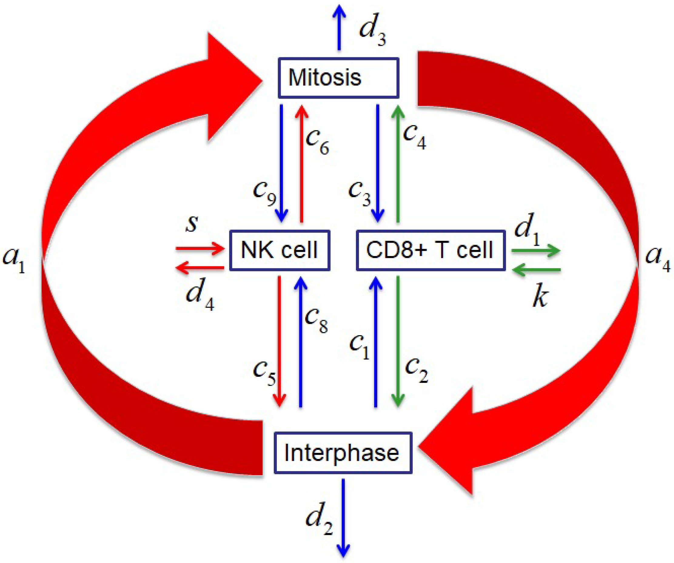
2. Construction of the Mathematical Model

The normal life cycle of the cell is divided into two phases: interphase and mitosis (M phase). The division activity corresponds to M phase while growth activity corresponds to interphase. The phases are exclusive in that a cell cannot be in the mitosis stage until the interphase is over and vice versa. Interphase is further divided into three sub-phases: $G_1$, S and $G_2$. $G_1$, the pre-synthesis phase, is a long period during which the cell is resting. This is followed by S, the synthesis phase, when DNA replication occurs. $G_2$ is another resting period for the cell, in anticipation of mitosis, when cells are divided to produce new cells. Mitosis is a brief process, typically an hour or less. The interphase constitutes more than $95\%$ of the duration of the cell cycle [26,27].

The division process from one part of the cell cycle to another depends on a variety of factors. These are growth, DNA replication, DNA integrity and cellular integrity. If the cell cycle detects abnormal activities, then it will prevent the cell from completing the cycle. This is called cell cycle checkpoint [27]. At the point when checkpoints are initiated, signals are sent to stop the progression of the cell cycle. These signals cause a delay until the defects are repaired [27].

Immune cells in the bone narrow and thymus undergo repeated cycling as part of their development. Cell cycle regulators are involved in the development of immune cells, partly as the machinery controlling the expansion and differentiation of the populations of immune cells. The cell cycle regulator is the core control system of the cell cycle. There are two main regulators of the cell cycle; positive cell regulator and negative cell regulator. Positive cell regulators perform tasks that advance the cell cycle to the next stage while negative regulators block the progression of the cell cycle. Emerging evidence has demonstrated that cell cycle regulators also directly control activities of several types of immune cells, in both the innate and adaptive immune systems.

Innate immunity refers to nonspecific defence mechanisms that can recognise foreign matter immediately without the requirement for previous priming. The cellular components of the innate immune system are neutrophil, macrophages, natural killer (NK) cells, dendritic cells (DCs), cytokines and innate lymphoid cells. Macrophages, NK cells and DCs are important in tumour recognition. NK cells play a key role by destroying abnormal cells before they replicate and grow.

Adaptive immunity is an immunity that occurs after exposure to an antigen, either from a pathogen or a vaccination. This part of the immune system is activated when the innate immune response is insufficient to control an infection. As part of the adaptive immunity, the activated CD$8^{+}$ Cytotoxic T Lymphocytes (CTL) play a crucial role in controlling the development of tumour cells. Activation of T cells occurs when the T cell receptors bind to the antigen peptides, on the major histocompatibility complex (MHC) class molecules, presented to them by the antigen-presenting cells, such dendritic cells or macrophages. CD$8^{+}$ T cells and NK cells are both cytotoxic effector cells of the immune system, but the recognition, specificity, sensitivity, and memory mechanisms are drastically different.

In this paper, four populations are considered. There are tumour cells in interphase, tumour cells during mitosis, NK and CD$8^{+}$ T cells as immune responses. A flow chart of the interaction model is given in Figure 1. Let $x\left(t\right)$ and $y\left(t\right)$ be the population of tumour cells during interphase and mitosis at time t respectively. $G_1+S+G_2$ is pre-mitotic phase called the interphase. $z\left(t\right)$ and $w\left(t\right)$ are the immune system population of NK and CD$8^{+}$ T cells at time t respectively. The assumptions used are based on previous researches and can be summarised as follows,

• The tumour growth mainly depends on the death rate and reproduction rate of the cells in the absent of immune cells [15,24,25].
• NK and CD$8^{+}$ T cells are expected to kill tumour cells [15,24,25].
• NK cells exist and are active, whether there are tumour cells or not [15,24,25].
• NK cell and CD$8^{+}$ T cells are inactivated after fighting the tumour cells [15,24,25].
• Tumour-specific CD$8^{+}$ T cell are initiated when tumour cells are detected [15].
• NK and CD$8^{+}$ T cells are assume to interact with cells from all phases

In this situation, the defining equations are

$$\begin{array}{cc}\hfill x^{\prime }& =2a_{4}y-c_{1}zx-d_{2}x-c_{7}xw-a_{1}x\left(t-\tau \right)\hfill \\ \hfill y^{\prime }& =a_{1}x\left(t-\tau \right)-d_{3}y-a_{4}y-c_{3}yz-c_{8}yw\hfill \\ \hfill z^{\prime }& =k+{\omega }_{1}z-c_{2}xz-c_{4}yz-d_{1}z\hfill \\ \hfill w^{\prime }& ={\omega }_{1}w-c_{5}xw-c_{6}yw-d_{4}w+rz\left(x+y\right)\hfill \end{array}$$

(1)

where

$${\omega }_1=\frac{\rho {\left(x+y\right)}^n}{\alpha +{(x+y)}^n}.$$

The terms $a_1$ and $a_4$ represent the proliferation rates at different stages of cell cycle and $c_i$ terms represents the number of cells that lost after fighting with tumour cells. The terms $d_{2}x$, $d_{3}y$, $d_{1}z$ and $d_{4}w$ in the model represent the natural death rates of cells.

The presence of tumour cells stimulates the immune cells which may be represented as non-linear growth of immune cells as $\frac{\rho {\left(x+y\right)}^n}{\alpha +{(x+y)}^n}$. Michaelis-Menten form has been chosen for this term, following other models in the literature [15,24,25]. The tumour cells stimulate the proliferation of tumour-specific effector cells. However, tumour-specific effector cells will reach saturation level at tumour population. The health of the immune system will determine the saturation level. Immune cells growth is assumed to be constant source rates k in the absent of tumour cells $(x=y=0)$. The term $rz\left(x+y\right)$ in Equation (1) represents the addition of tumour-specific $\mathrm{CD}{8}^{+}$ T cells that are simulated by the interaction between NK and tumour cells.

$\alpha$, $\rho$ and n are parameters in the Michaelis–Menten form, where $\rho$ indicates the maximum immune responses to combat the tumour cell. If the tumour cells $\left(x+y\right)$ level is equal to $\alpha$, then the immune response is half of its maximum value $\rho$. In this model, the value of $n=3$ is taken from [28]. When n is large, it takes a longer time for the tumour to be recognised by the immune system and once the immune system becomes aware of this agent it begins the production of immune cells. The tumour cells stay in interphase for a certain time $\tau$, before entering mitosis phase. Mitosis is a very short stage, it is felt that a delay is not necessary. Mitosis is assumed to be the growth of tumour cell population and represented by parameters $a_1$, $a_4$ and $\tau$. The term $xz$, $xw$, $yz$ and $yz$ represent the cell loss during the competition with other cells.

Parameter Values

To complete the development of the mathematical model, we define values for the parameters and initial conditions. We found that there were large ranges in the parameter choices between studies, and we chose the most suitable value for the proposed model. The values are given in

Table 1. Parameter values.

Parameter	Description	Estimated Value/Range	Source
$a_1$	Cell that enter interphase	0–1 day${}^{-1}$	[25,28]
$a_4$	Cell that enter mitosis	0–1 day${}^{-1}$	[25,28]
$d_1$	Natural death rate of NK cell	$4.12\times {10}^{-2}$ day${}^{-1}$ cell${}^{-1}$	[29]
$d_2$	Natural death rate of tumour cell	0–1 day${}^{-1}$	[25,28]
	at interphase
$d_3$	Natural death rate of tumour cell	0–1 day${}^{-1}$	[25,28]
	at mitosis
$d_4$	Natural death rate of CD$8^{+}$ T cell	$2.0\times {10}^{-2}$ day${}^{-1}$ cell${}^{-1}$	[29]
$c_1$	Rate at which NK cell destroy	$1.3\times {10}^{-7}$ day${}^{-1}$ cell${}^{-1}$	[29]
	tumour at interphase
$c_2$	Loses due to encounter with NK cell	$1.3\times {10}^{-7}$ day${}^{-1}$ cell${}^{-1}$	[29]
	at interphase
$c_3$	Rate at which NK cell destroy	$1.3\times {10}^{-7}$ day${}^{-1}$ cell${}^{-1}$	[29]
	tumour at mitosis
$c_4$	Loses due to encounter with NK cell	$1.2\times {10}^{-9}$ day${}^{-1}$ cell${}^{-1}$	[29]
	at mitosis
$c_5$	Loses due to encounter with CD$8^{+}$ T cell	$1.3\times {10}^{-7}$ day${}^{-1}$ cell${}^{-1}$	[29]
	at interphase
$c_6$	Loses due to encounter with CD$8^{+}$ T cell	$1.3\times {10}^{-7}$ day${}^{-1}$ cell${}^{-1}$	[29]
	at mitosis
$c_7$	Rate at which CD$8^{+}$ T cell destroy	$1.2\times {10}^{-9}$ day${}^{-1}$ cell${}^{-1}$	[29]
	tumour at interphase
$c_8$	Rate at which CD$8^{+}$ T cell destroy	$1.3\times {10}^{-7}$ day${}^{-1}$ cell${}^{-1}$	[29]
	tumour at mitosis
k	Constant source of NK cell	$1.3\times {10}^4$ day${}^{-1}$ cell${}^{-1}$	[25,28]
r	Rate at which tumour-specific	$1.1\times {10}^{-7}$ day${}^{-1}$ cell${}^{-1}$	[28]
	CD$8^{+}$ T cell are stimulated
$\rho$	Proportion of the growth of lymphocytes	$2.5\times {10}^{-2}$ day${}^{-1}$	[25,28]
	due to stimulus by tumour cell
$\alpha$	Steepness coefficient of the NK	$2.02\times {10}^{-7}$ day${}^{-1}$ cell${}^{-1}$	[25,28]
	and CD$8^{+}$ T cells recruitment curve

.

3. Stability Analysis

Stability of the system is determined by linearising the system about the equilibrium points. The system in (1) can have many fixed points depending on the parameter values. In this paper, we consider that two equilibrium points exist. There is a tumour-free fixed point with a positive immune level and a tumour fixed point with a positive immune level.

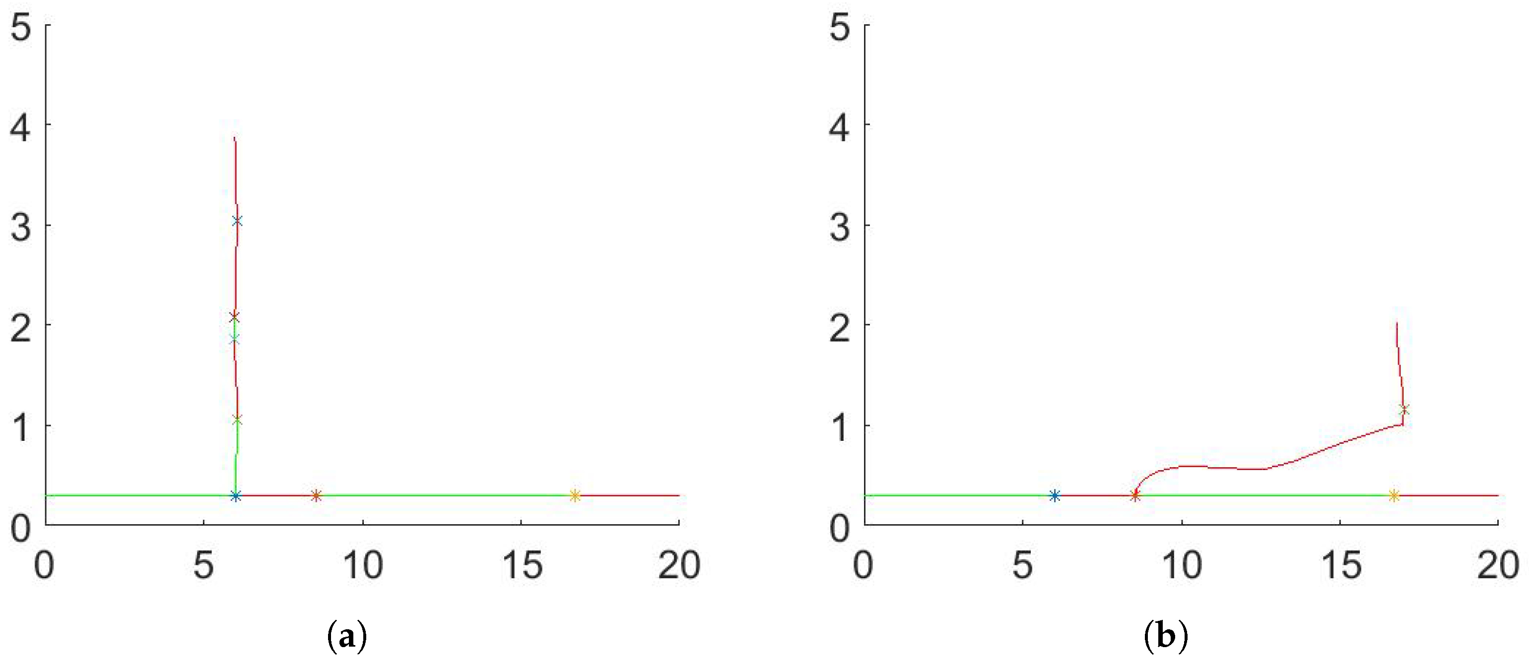
3.1. Steady State and Stability Result

It is important to look at the long-term behaviour of tumour cell populations. In this section, we inspect the equilibria and stability properties of system (1). There are two steady states of $E_i$ existing in the form of $x^{*},y^{*},z^{*},w^{*}$, where $i=0,1$:

(a)

$E_0=(0,0,\frac{k}{d_1},0)$

(b)

$E_1=(x^{*},y^{*},z^{*},w^{*})$

To examine the stability and local behavior of each equilibrium, we make use of the variational matrix of system (1). The matrices A and B are given by

$$A=\left[\begin{array}{cccc}{A}_1& 2a_4& -c_1{x}^{*}& -c_7{x}^{*}\\ 0& A_2& -c_3{y}^{*}& -c_8{y}^{*}\\ A_3& A_4& A_5& 0\\ A_6& A_7& r(x^{*}+y^{*})& A_8\end{array}\right],B=e^{-\tau }\left[\begin{array}{cccc}-a_1& 0& 0& 0\\ a_1& 0& 0& 0\\ 0& 0& 0& 0\\ 0& 0& 0& 0\end{array}\right]$$

(2)

where

$$\begin{array}{cc}\hfill A_1& =-(c_1{z}^{*}+d_2+c_7{w}^{*})\hfill \\ \hfill A_2& =-(d_3+a_4+c_3{z}^{*}+c_8{w}^{*})\hfill \\ \hfill A_3& =\frac{3\alpha \rho z^{*}{(x^{*}+y^{*})}^2}{{(\alpha +{(x^{*}+y^{*})}^3)}^2}-c_2{z}^{*}\hfill \\ \hfill A_4& =\frac{3\alpha \rho z^{*}{(x^{*}+y^{*})}^2}{{(\alpha +{(x^{*}+y^{*})}^3)}^2}-c_4{z}^{*}\hfill \\ \hfill A_5& =\frac{\rho {(x^{*}+y^{*})}^3}{\alpha +{(x^{*}+y^{*})}^3}-c_2{x}^{*}-c_4{y}^{*}-d_1\hfill \\ \hfill A_6& =\frac{3\alpha \rho w^{*}{(x^{*}+y^{*})}^2}{{(\alpha +{(x^{*}+y^{*})}^3)}^2}-c_5{w}^{*}+r{z}^{*}\hfill \\ \hfill A_7& =\frac{3\alpha \rho w^{*}{(x^{*}+y^{*})}^2}{{(\alpha +{(x^{*}+y^{*})}^3)}^2}-c_6{w}^{*}+r{z}^{*}\hfill \\ \hfill A_8& =\frac{\rho {(x^{*}+y^{*})}^3}{\alpha +{(x^{*}+y^{*})}^3}-c_5{x}^{*}-c_6{y}^{*}-d_4\hfill \end{array}$$

3.2. Stability Result of Tumour-Free Equilibrium Point, $E_0$

To examine the local stability of tumour-free equilibrium $E_0$ (case for $\tau =0$), the variational matrix or the Jacobian becomes

$$\left[\begin{array}{cccc}-(c_1\frac{k}{d_1}+d_2+a_1)& 2a_4& 0& 0\\ a_1& -(d_3+a_4+c_3\frac{k}{d_1})& 0& 0\\ c_2\frac{k}{d_1}& 0& -d_1& 0\\ r\frac{k}{d_1}& r\frac{k}{d_1}& 0& -d_4\end{array}\right].$$

(3)

Clearly $\lambda =-d_1$ and $-d_4$ are eigenvalues, the remaining eigenvalues are given as the solutions to the characteristic equation

$${\lambda }^2+{\alpha }_0\lambda +{\alpha }_1=0,$$

(4)

where

$$\begin{array}{cc}\hfill {\alpha }_0& =(a+a_1)+(d+a_4)\hfill \\ \hfill {\alpha }_1& =(a+a_1)(d+a_4)-2a_1{a}_4\hfill \\ \hfill a& =c_1\frac{k}{d_1}+d_2\hfill \\ \hfill d& =c_3\frac{k}{d_1}+d_3\hfill \end{array}$$

${\alpha }_0$ is always positive. By Routh Hurwitz criteria, sufficient and necessary conditions for $\lambda$ to become negative real part is ${\alpha }_1>0$ such that

$$(a+a_1)(d+a_4)>2a_1{a}_4.$$

(5)

Different values of $a_1$, $a_4$, a and d will affect the stability of the fixed point of the system. a represents the total cell lost at the interphase where d represents the total cell lost at the mitosis. The cell lost is the summation of natural death (apoptosis) of the tumour cell and the tumour cells that are killed by the immune system in each phase of the cell cycle. Based on the condition in (5), the tumour would be defeated when there is no immune system interaction since the death rates dominate the growth rate. The literature shows that the rate of natural death (apoptosis) of the tumour cell is very low in the malignant tumour. Hence, we consider the death rate of tumour cells killed by the immune system is higher than the natural death rate of the tumour cells, $c_1\frac{k}{d_1}>d_2$ and $c_3\frac{k}{d_1}>d_3$. The value of a and d should be higher than proliferation rate of the tumour cell, $a_1$ and $a_4$, so that the tumour growth can be diminished. In the absence of immune response, these two parameters should be in control in order to maintain the growth of the tumour. However, as far as the immune responses are concerned, it greatly helps to suppress tumour growth by inhibiting their outgrowth. Villasana [24] and Liu [25] have focused on involving one immune response with results showing that the immune cell can suppress the tumour growth. From the results, we extend the model by adding another immune response since there are two types of immune system in the human body, i.e., innate and adaptive immune system. NK cell is a part of the innate system and the first line of defence against viruses and tumours. Once NK cells detect a foreign cell (tumour cell), they will directly attack the latter and give an alert signal to T cells (CD$8^{+}$ T cell) and generate tumour-specific CD$8^{+}$ T cell, which is represented by CD$8^{+}$ T cell in the presented model. Tumour-specific CD$8^{+}$ T cell is only present in the presence of a tumour cell and helps CD$8^{+}$ T cell to kill the tumour cell. By including both immune responses from both immune systems, the model is more realistic.

If $(a+a_1)(d+a_4)<2a_1{a}_4$, a low death rate of the NK cell, a high NK cell production rate, k or a high immunotherapy effectiveness is necessary for tumour eradication.

It is indeed practical to have a stability conditions in term of immune parameter, k as that can be controlled from the outside, for example with chemotherapeutic treatments.

Now the effect of the delay is added in the system. As the delay is varied the conditions of the tumour growth changes. When the delay is positive, the the characteristic equation for the linearised equation about the $E_0$ is given by

$$\left[\begin{array}{cccc}\lambda +a& -2a_4& 0& 0\\ 0& \lambda +d& 0& 0\\ c_2\frac{k}{d_1}& c_4\frac{k}{d_1}& \lambda +d_1& 0\\ c_5\frac{J}{d_4}& c_6\frac{J}{d_4}& 0& \lambda +d_4\end{array}\right]\left[\begin{array}{c}x\\ y\\ z\\ w\end{array}\right]-\left[\begin{array}{cccc}-a_1& 0& 0& 0\\ a_1& 0& 0& 0\\ 0& 0& 0& 0\\ 0& 0& 0& 0\end{array}\right]\left[\begin{array}{c}{x}_{\tau }\\ y_{\tau }\\ z_{\tau }\\ w_{\tau }\end{array}\right]=0,$$

$$F\left(\lambda \right)=\left(\lambda +d_1\right)\left(\lambda +d_4\right)\left[\left({\lambda }^2+\left(d+a\right)\lambda +da\right)+e^{-\lambda \tau }\left(a_1\lambda +a_{1}d-2a_1{a}_4\right)\right]$$

Clearly ${\lambda }_1=-d_1$ and ${\lambda }_2=-d_4$ are negative real roots. Then, the stability of $E_0$ is determined by the distribution of the roots of equation

$$\left({\lambda }^2+\left(d+a\right)\lambda +da\right)+e^{-\lambda \tau }\left(a_1\lambda +a_{1}d-2a_1{a}_4\right)=0$$

(6)

Now substituting $\lambda =i\omega$ where $\omega \in \mathbb{R}$. We obtained the system transcendental equations to determine $\omega$ and $\tau$.

$$P_1\left(i\omega \right)+P_2\left(i\omega \right)e^{-i\omega \tau }=0$$

(7)

We break the polynomial up into its real and imaginary parts, and write the exponential in terms of trigonometric functions to obtain

$$R_1\left(\omega \right)+i{Q}_1\left(\omega \right)+(R_2\left(\omega \right)+i{Q}_2\left(\omega \right))cos\left(\omega \tau \right)-isin\left(\omega \tau \right)=0$$

(8)

where

$$\begin{array}{c}\hfill R_1\left(\omega \right)=-{\omega }^2+da\\ \hfill Q_1\left(\omega \right)=(d+a)\omega \\ \hfill R_2\left(\omega \right)=a_{1}d-2a_1{a}_4\\ \hfill Q_2\left(\omega \right)=a_1\omega .\end{array}$$

(9)

In order for (8) to hold, both the real and imaginary part must be 0, so we obtain the pair of equations

$$\begin{array}{c}\hfill (-{\omega }^2+da)+(a_{1}d-2a_1{a}_4)cos\left(\omega \tau \right)+a_1\omega sin\left(\omega \tau \right)=0\\ \hfill (d+a)\omega -(a_{1}d-2a_1{a}_4)sin\left(\omega \tau \right)+a_1\omega cos\left(\omega \tau \right)=0,\end{array}$$

(10)

which can be rewritten as

$$\begin{array}{c}\hfill -(-{\omega }^2+da)=(a_{1}d-2a_1{a}_4)cos\left(\omega \tau \right)+a_1\omega sin\left(\omega \tau \right),\\ \hfill (d+a)\omega =(a_{1}d-2a_1{a}_4)sin\left(\omega \tau \right)-a_1\omega cos\left(\omega \tau \right).\end{array}$$

(11)

Squaring each equation and summing the results yields

$${(-{\omega }^2+da)}^2+{\left((d+a)\omega \right)}^2={(a_{1}d-2a_1{a}_4)}^2+{\left(a_1\omega \right)}^2.$$

(12)

Solving the equation we obtain the polynomial

$${\omega }^4+({(d+a)}^2-2ad-a_1^2){\omega }^2+d^2{a}^2-a_1^2{d}^2+4d{a}_1^2{a}_4-4a_1^2{a}_4^2=0.$$

(13)

By letting $\mu ={\omega }^2$, the equation becomes a quadratic with roots given by

$$S\left(\mu \right)={\mu }^2+{\beta }_0\mu +{\beta }_1=0.$$

(14)

where

$$\begin{array}{c}\hfill {\beta }_0=(d^2+a^2-a_1^2)\\ \hfill {\beta }_1=d^2{a}^2-a_1^2{(d-2a_4)}^2.\end{array}$$

Equation (14) has a positive real root in two circumstances. Since the lead coefficient is positive, if ${\beta }_1<0$ then there is a single positive real root. If ${\beta }_1>0$, the root of (14) are

$$\mu =\frac{\left(-{\beta }_0\pm \sqrt{{\left({\beta }_0\right)}^2-4{\beta }_1}\right)}{2},$$

(15)

and there is a simple positive root if and only if ${\beta }_0<0$ and ${\beta }_0^2-4{\beta }_1>0$. Thus, we can conclude.

Theorem 1.

A steady state with characteristic Equation (6) is stable in the absence of delay, and becomes unstable with increasing delay if and only if

1.

$(a+a_1)+(d+a_4)>0$ and $(a+a_1)(d+a_4)>2a_1{a}_4$, and

2.

either $a^2{d}^2<a_1^2{(d-2a_4)}^2$, or $a^2{d}^2>a_1^2{(d-2a_4)}^2$, $d^2+a^2<a_1^2$ and $(d^2+a^2-a_1^2)>4a^2{d}^2-4a_1^2{(d-2a_4)}^2$.

Noted that we are only interested in $\omega \in \mathbb{R}$, and thus if all of the real roots of (14) are negative, we will have shown that there can be no simultaneous solution ${\omega }^{*}$ of (11). Conversely, if there is a positive real root ${\mu }^{*}$ to (14), there is a delay $\tau$ corresponding to ${\omega }^{*}=\pm \sqrt{{\mu }^{*}}$, which solves the equation in (11).

Now, suppose that (14) has a positive real root. Then, there exists a positive root, ${\omega }_0$, satisfying (11) and hence the characteristic equation has a pair of imaginary roots $\pm i{\omega }_0$. Eliminating $sin\left(\omega \tau \right)$ and we obtain the expression for the time delay as

$${\tau }_n^{*}=\frac{1}{{\omega }_0}arccos\left[\frac{-\left(a_{1}d-2a_1{a}_4\right)\left({\omega }_0^2-da\right)-\left((d+a){\omega }_0\right)\left(a_1{\omega }_0\right)}{{\left(a_{1}d-2a_1{a}_4\right)}^2+{\left(a_1{\omega }_0\right)}^2}\right]+\frac{2n\pi }{{\omega }_0},$$

(16)

where for $\tau =0$ the equilibrium point $E_0$ is stable. When $\tau ={\tau }_0$, the characteristic equation has a imaginary root where bifurcation will occurs. As $\tau >0$, there is at least one root with positive real part.

The tumour conditions are represented by the region in Figure 2. Assume that there is no natural death of the tumour cell, $d_2=d_3=0$. The resulting curves are obtained when the parameters $a_4=0.5$, $c_1=c_3=c_7=c_8=0.02$, $c_2=c_4=c_5=c_6=0.008$, $k=0.41$ and $d_1=0.028$. The curves show the regions of growth, decay and stability switching. In the absence of delay, $\tau =0$, tumour growth is as shown in Figure 3. However, when $\tau$ increases, the region of tumour decay starts to change and becomes smaller. In the case $\tau >0$, tumour growth remains at the same region (R-I), while the decay region is subdivided into four regions including the regions of stability switching. For $\tau >0$, tumour regions are given by R-II and R-IV and as $\tau$ increases the stability switching occurs at R-III and R-V as shown in Figure 2.

Stability switching is very important in cancer chemotherapy. Cycle-specific drugs perform the primary action during specific phase of the cycle, i.e., interphase and M phase. They trap the tumour cell at some points and prevent the cell from continuing their cycle. Then, the cell will die due to natural causes and not undergo mitosis process. As a result, tumour growth stops. However, the trapping cells may have an adverse effect since some tumours can inhibit the immune system and become active. The active cell will enter the mitosis phase and continue to grow.

3.3. Stability Result of Tumour Equilibrium Point with Immune Responses $E_1$

Let $\tau =0$, then the linearised system of (1) at $E_1$ generates a characteristic equation

$${\lambda }^4+\left(B_0+C_0\right){\lambda }^3+\left(B_1+C_1\right){\lambda }^2+\left(B_2+C_2\right)\lambda +B_3+C_3=0.$$

(17)

where

$$\begin{array}{cc}\hfill B_0& =-(A_1+2a_4+c_1{x}^{*}+c_7{x}^{*})\hfill \\ \hfill B_1& =(A_5+A_2+A_1)A_8+A_7{c}_8{y}^{*}+A_6{c}_7{x}^{*}+(A_1+A_2)A_5+A_4{c}_3{y}^{*}+A_3{c}_1{x}^{*}\hfill \\ \hfill & +A_1{A}_2\hfill \\ \hfill B_2& =-A_3{A}_2{c}_1{x}^{*}+2A_3{a}_4{c}_3{y}^{*}-A_1{A}_4{c}_3{y}^{*}-A_1{A}_2{A}_5-A_6{A}_2{c}_7{x}^{*}\hfill \\ \hfill & -A_6{A}_5{c}_7{x}^{*}+2a_4{c}_8{A}_6{y}^{*}-A_1{A}_7{c}_8{y}^{*}-A_7{A}_5{c}_8{y}^{*}+A_6{c}_1{x}^{*}r(x^{*}+y^{*})\hfill \\ \hfill & +A_7{c}_3{y}^{*}r(x^{*}+y^{*})-A_1{A}_2{A}_8-A_3{A}_8{c}_1{x}^{*}-A_4{A}_8{c}_3{y}^{*}-A_1{A}_4{A}_8\hfill \\ \hfill & -A_2{A}_5{A}_8\hfill \\ \hfill B_3& =A_6{A}_4{c}_3{y}^{*}{c}_7{x}^{*}-A_3{A}_7{c}_3{y}^{*}{c}_7{x}^{*}+A_6{A}_2{A}_5{c}_7{x}^{*}\hfill \\ \hfill & -A_6{A}_4{c}_1{x}^{*}{c}_8{y}^{*}+A_3{A}_7{c}_1{x}^{*}{c}_8{y}^{*}-2A_6{A}_5{a}_4{c}_8{y}^{*}+A_1{A}_7{A}_5{c}_8{y}^{*}\hfill \\ \hfill & -A_6{A}_2{c}_1{x}^{*}r(x^{*}+y^{*})-A_1{A}_7{c}_3{y}^{*}r(x^{*}+y^{*})+2A_6{a}_4{c}_3{y}^{*}r(x^{*}+y^{*})\hfill \\ \hfill & +A_3{A}_2{A}_8{c}_1{x}^{*}-2A_3{A}_8{a}_4{c}_3{y}^{*}+A_1{A}_4{A}_8{c}_3{y}^{*}+A_1{A}_2{A}_5{A}_8\hfill \\ \hfill C_0& =-a_1\hfill \\ \hfill C_1& =a_1(A_8+A_5+A_2-2a_4)\hfill \\ \hfill C_2& =a_1(A_4{c}_1{x}^{*}-A_3{c}_3{y}^{*}+2a_4{A}_5-A_2{A}_5-(A_7+A_2+A_5)A_8)\hfill \\ \hfill C_3& =a_1(-A_7{A}_5{c}_7{x}^{*}+A_7{A}_5{c}_8{y}^{*}+A_7{c}_1{x}^{*}r(x^{*}+y^{*})-A_7{c}_3{y}^{*}r(x^{*}+y^{*})\hfill \\ \hfill & -A_4{A}_8{c}_3{y}^{*}-2a_4{A}_5{A}_8+A_2{A}_5{A}_8)\hfill \end{array}$$

The steady state is stable if the real part of roots of the characteristic polynomial (17) are negative. By the Routh–Hurwitz theorem, it can be shown that the necessary and sufficient conditions for the system are as follows:

Theorem 2.

Consider system as in (1). For the system without delay $(\tau =0)$, the steady state is locally asymptotically stable if

a.

$\left(B_0+C_0\right)>0$,

b.

$\left(B_2+C_2\right)>0$

c.

$\left(B_3+C_3\right)>0$, and

d.

$\left({\displaystyle \prod _{i=0}^{n=3}}{B}_i+C_i\right)-\left({\left(B_2+C_2\right)}^2+{\left(B_0+C_0\right)}^2\left(B_3+C_3\right)\right)>0$.

Proof. 

Consider system (1) with $\tau =0$ holds. Assume the steady state of the system is locally asymptotically stable. Then the system (1) is said to be stable if and only if the roots of its characteristic equation have negative real parts. The characteristic equation of system (1) with $\tau =0$ is Equation (17). All the roots of (17) have negative real part if (17) satisfies conditions a, b, c and d.   □

In case of positive delay ($\tau >0$), the system in (1) is linearised around the fixed point $E_1$ and the characteristic equation is

$${\lambda }^4+B_0{\lambda }^3+B_1{\lambda }^2+B_2\lambda +B_3+\left(C_0{\lambda }^3+C_1{\lambda }^2+C_2\lambda +C_3\right)e^{-\lambda \tau }=0.$$

(18)

Now substituting $\lambda =i\omega$ where $\omega$ is positive in the characteristic equation. We obtained the system transcendental equations to determine $\omega$ and $\tau$.

$$P_1\left(i\omega \right)+P_2\left(i\omega \right)e^{-i\omega \tau }=0$$

(19)

We break the polynomial up into its real and imaginary parts, and write the exponential in terms of trigonometric functions to obtain

$$R_1\left(\omega \right)+i{Q}_1\left(\omega \right)+(R_2\left(\omega \right)+i{Q}_2\left(\omega \right))cos\left(\omega \tau \right)-isin\left(\omega \tau \right)=0$$

(20)

where

$$\begin{array}{c}\hfill R_1\left(\omega \right)=-{\omega }^4-B_1{\omega }^2+B_3,\\ \hfill Q_1\left(\omega \right)=-B_0{\omega }^3+B_2\omega ,\\ \hfill R_2\left(\omega \right)=-C_1{\omega }^2+C_3,\\ \hfill Q_2\left(\omega \right)=-C_0{\omega }^3+C_2\omega .\end{array}$$

(21)

In order for (20) to hold, both the real and imaginary part must be 0, so we obtain the pair of equations

$$\begin{array}{c}\hfill (-{\omega }^4-B_1{\omega }^2+B_3)+(-C_1{\omega }^2+C_3)cos\left(\omega \tau \right)+(-C_0{\omega }^3+C_2\omega )sin\left(\omega \tau \right)=0\\ \hfill (-B_0{\omega }^3+B_2\omega )-(-C_1{\omega }^2+C_3)sin\left(\omega \tau \right)+(-C_0{\omega }^3+C_2\omega )\omega cos\left(\omega \tau \right)=0,\end{array}$$

(22)

which can be rewritten as

$$\begin{array}{c}\hfill -(-{\omega }^4-B_1{\omega }^2+B_3)=(-C_1{\omega }^2+C_3)cos\left(\omega \tau \right)+(-C_0{\omega }^3+C_2\omega )sin\left(\omega \tau \right)\\ \hfill (-B_0{\omega }^3+B_2\omega )=(-C_1{\omega }^2+C_3)sin\left(\omega \tau \right)-(-C_0{\omega }^3+C_2\omega )\omega cos\left(\omega \tau \right),\end{array}$$

(23)

Squaring each equation and summing the results yields

$${(-{\omega }^4-B_1{\omega }^2+B_3)}^2+{(-B_0{\omega }^3+B_2\omega )}^2={(-C_1{\omega }^2+C_3)}^2+{(-C_0{\omega }^3+C_2\omega )}^2.$$

(24)

Solving the equation we obtain the polynomial

$${\omega }^8+A{\omega }^6+B{\omega }^4+C{\omega }^2+D=0$$

where

$$\begin{array}{cc}\hfill A& =B_0^2-2B_1-C_0^2\hfill \\ \hfill B& =B_1^2-2B_0{B}_2-2B_3-C_1^2+2C_0{C}_2\hfill \\ \hfill C& =B_2^2+2B_1{B}_3-C_2^2+2C_1{C}_3\hfill \\ \hfill D& =B_3^2-C_3^2.\hfill \end{array}$$

(25)

By letting $\mu ={\omega }^2$, the equation becomes a polynomial with roots given by

$${\mu }^4+A{\mu }^3+B{\mu }^2+C\mu +D=0.$$

(26)

Noted that we are only interested in $\omega \in \mathbb{R}$, and thus if all of the real roots of (26) are negative, we will have shown that there can be no simultaneous solution ${\omega }^{*}$ of (22). Conversely, if there is a positive real roots ${\mu }^{*}$ to (26), there is a delay $\tau$ corresponding to ${\omega }^{*}=\pm \sqrt{{\mu }^{*}}$ which solve equation in (22).

Now, suppose that (26) has a positive real root. Then there exist a positive ${\omega }_0$, satisfying (22) and hence the characteristic equation has a pair of imaginary roots $\pm i{\omega }_0$. Eliminating $sin\left(\omega \tau \right)$, we obtain the expression for the time delay as

$$\begin{array}{cc}\hfill & {\tau }_0=\frac{1}{{\omega }_0}arccos\hfill \\ \hfill & \left\{\frac{-\left(-C_1{\omega }_0^2+C_3\right)\left(-{\omega }_0^4-B_1{\omega }_0^2+B_3\right)-\left(-B_0{\omega }_0^3+B_2{\omega }_0\right)}{{\left(-C_1{\omega }_0^2+C_3\right)}^2+\left(-C_0{\omega }_0^3+C_2{\omega }_0\right)}\right\}+\frac{2n\pi }{{\omega }_0},\hfill \end{array}$$

(27)

where for $\tau =0$ the steady state $E_0$ is stable. When $\tau ={\tau }_0$, the characteristic Equation (18) has a pair of imaginary roots, ${\lambda }^{*}=\pm i\sqrt{{\mu }^{*}}$, where bifurcation will occurs. As $\tau >{\tau }_0$, there is at least one root with positive real part which means that at least one stability switching occurred. If there is no positive root, then the system does not have bifurcation and cannot lead to a stability switching.

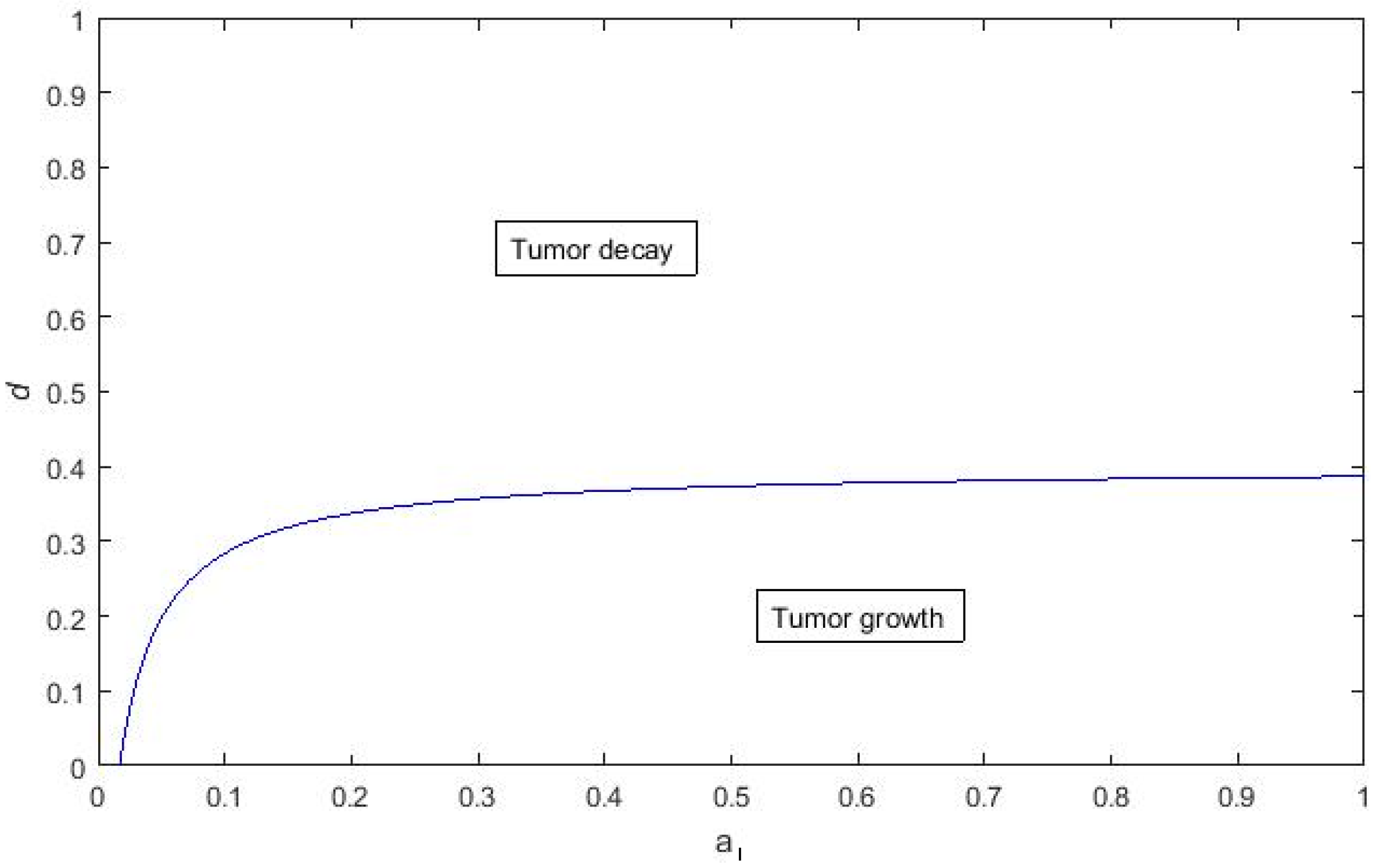
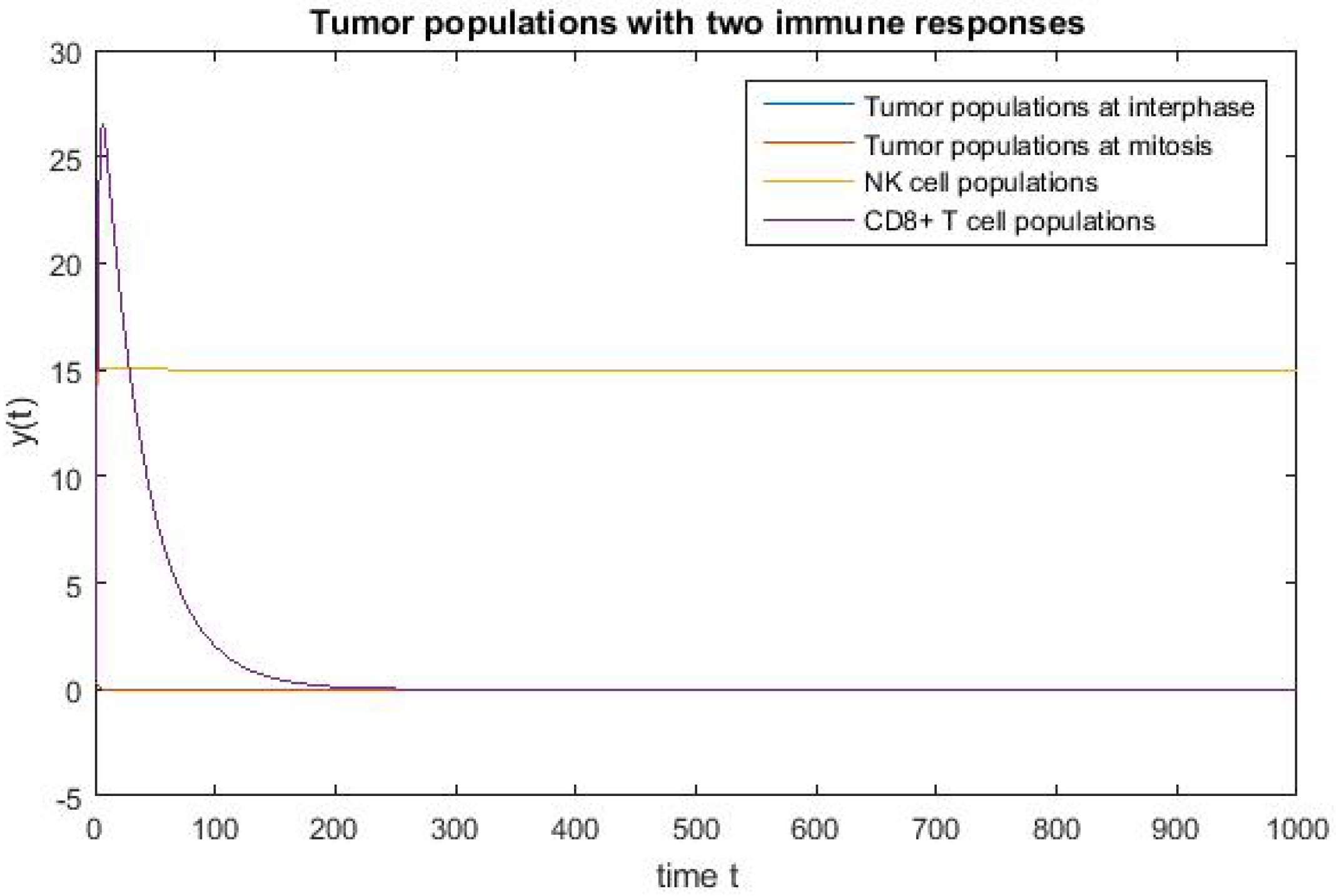
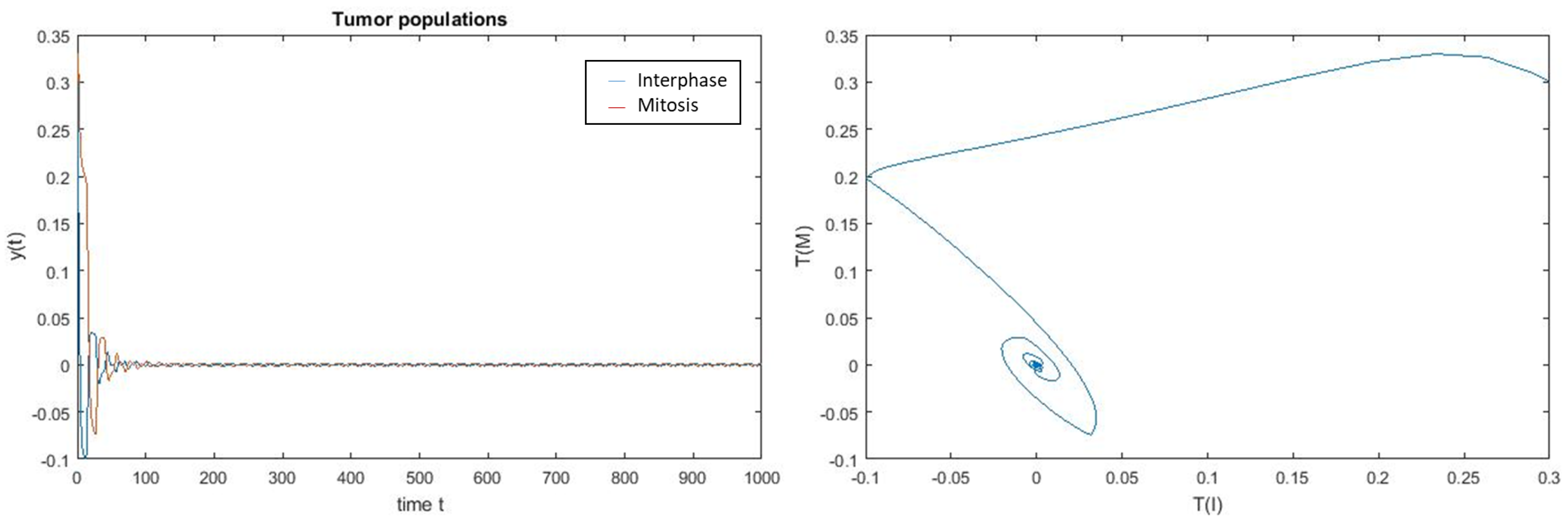
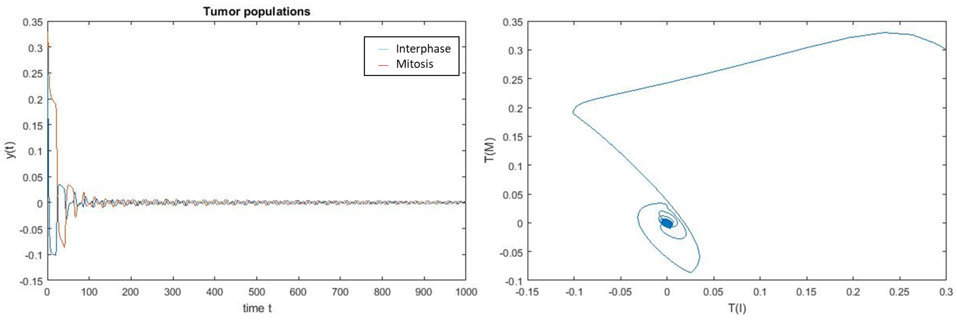
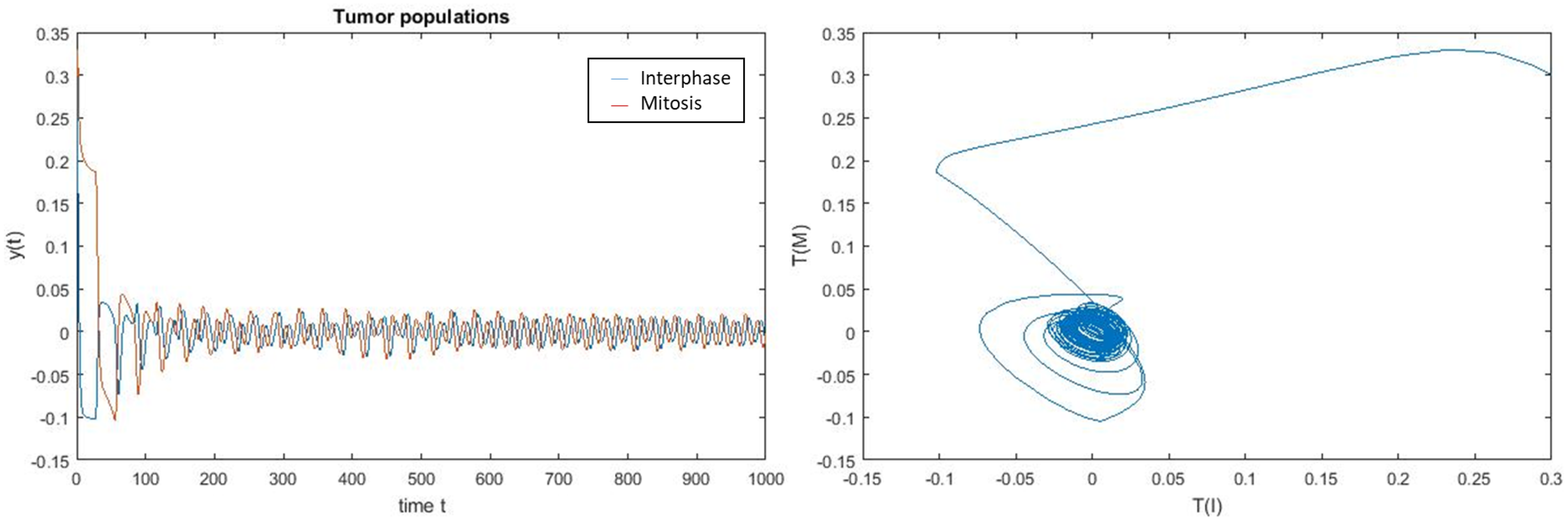
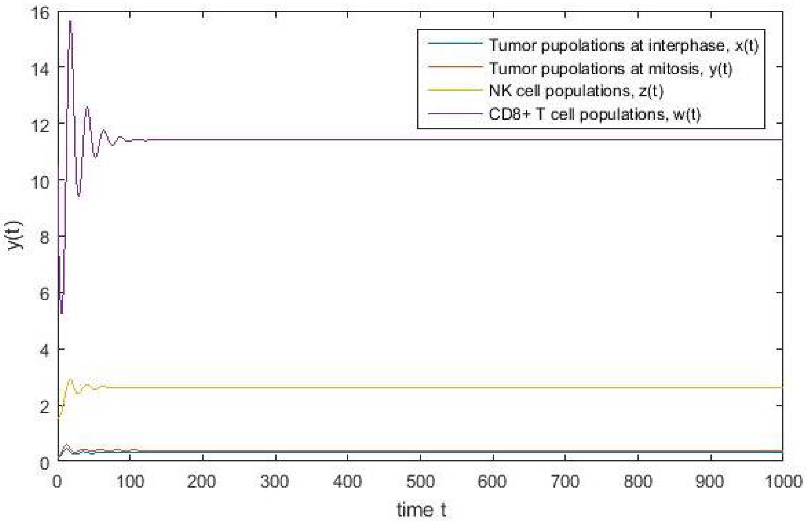
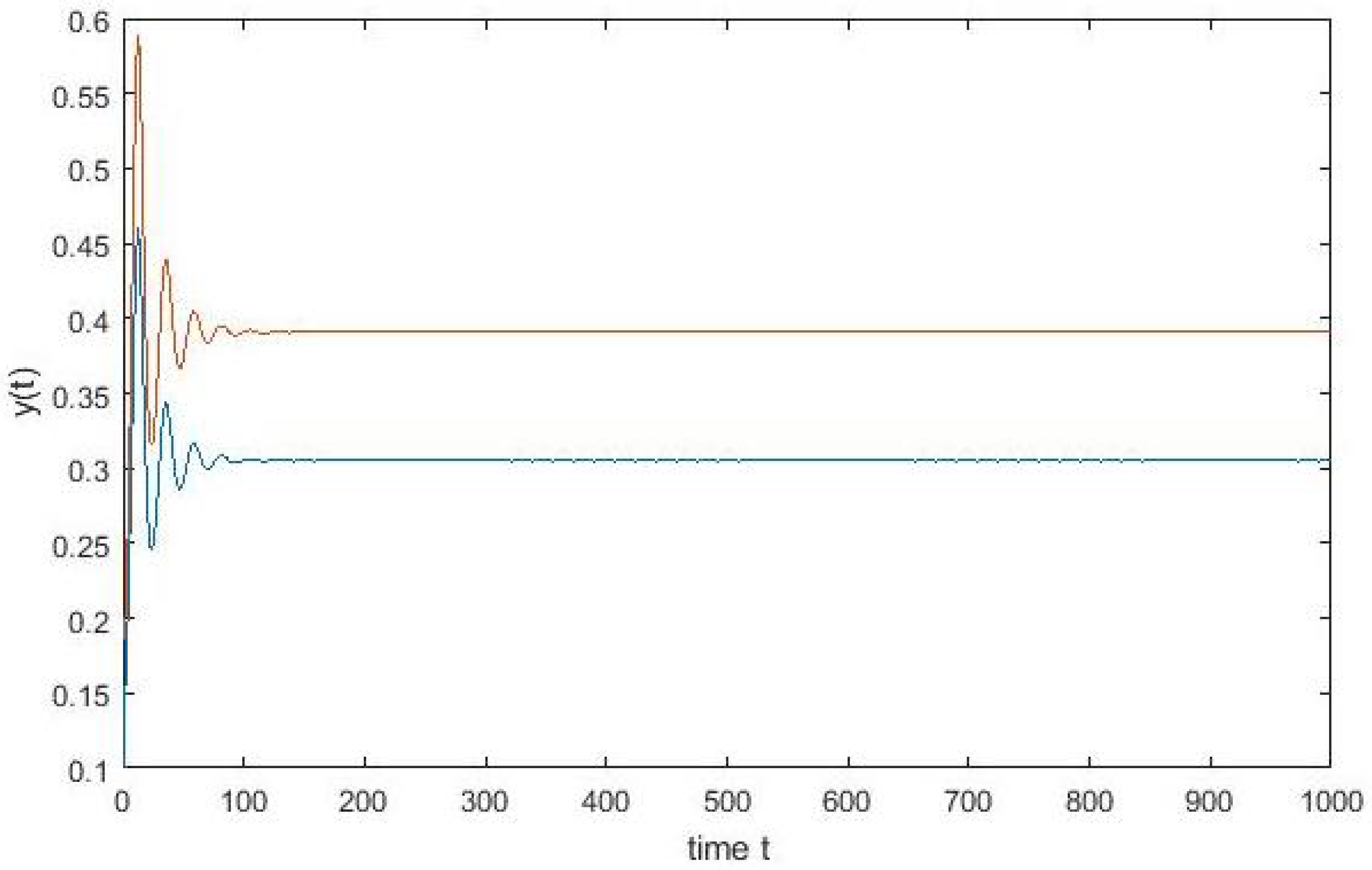
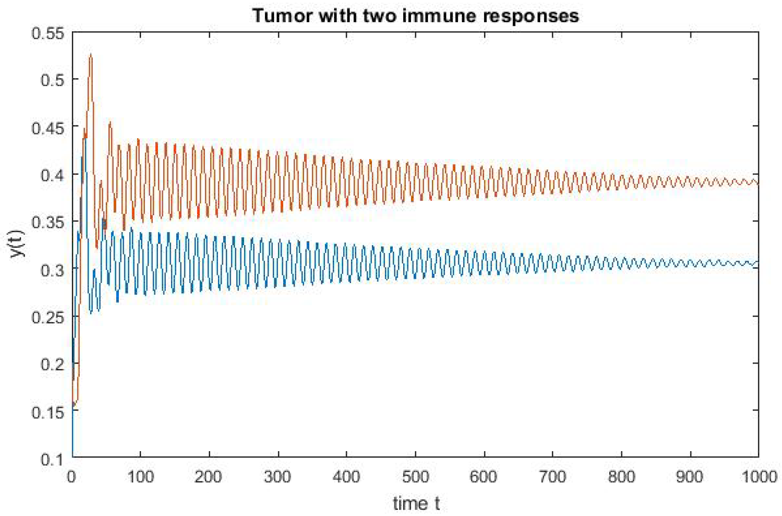
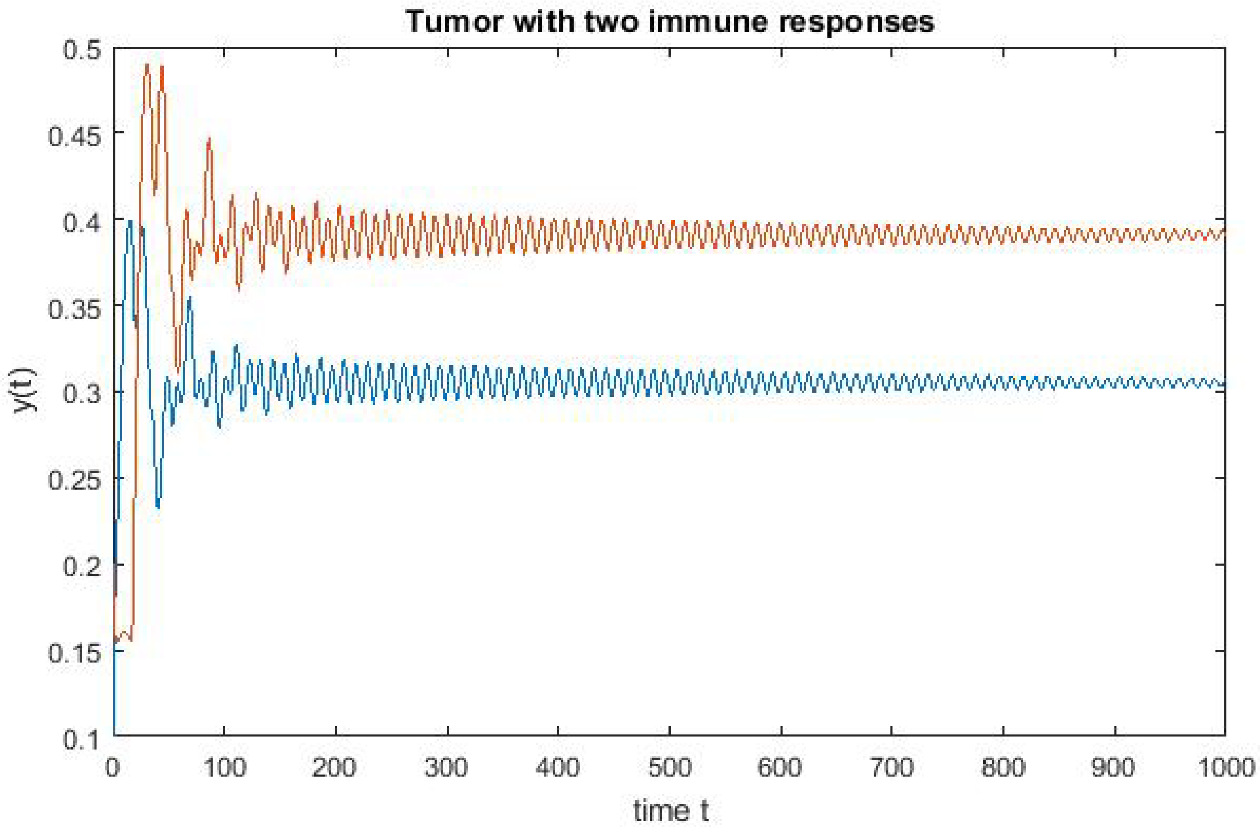
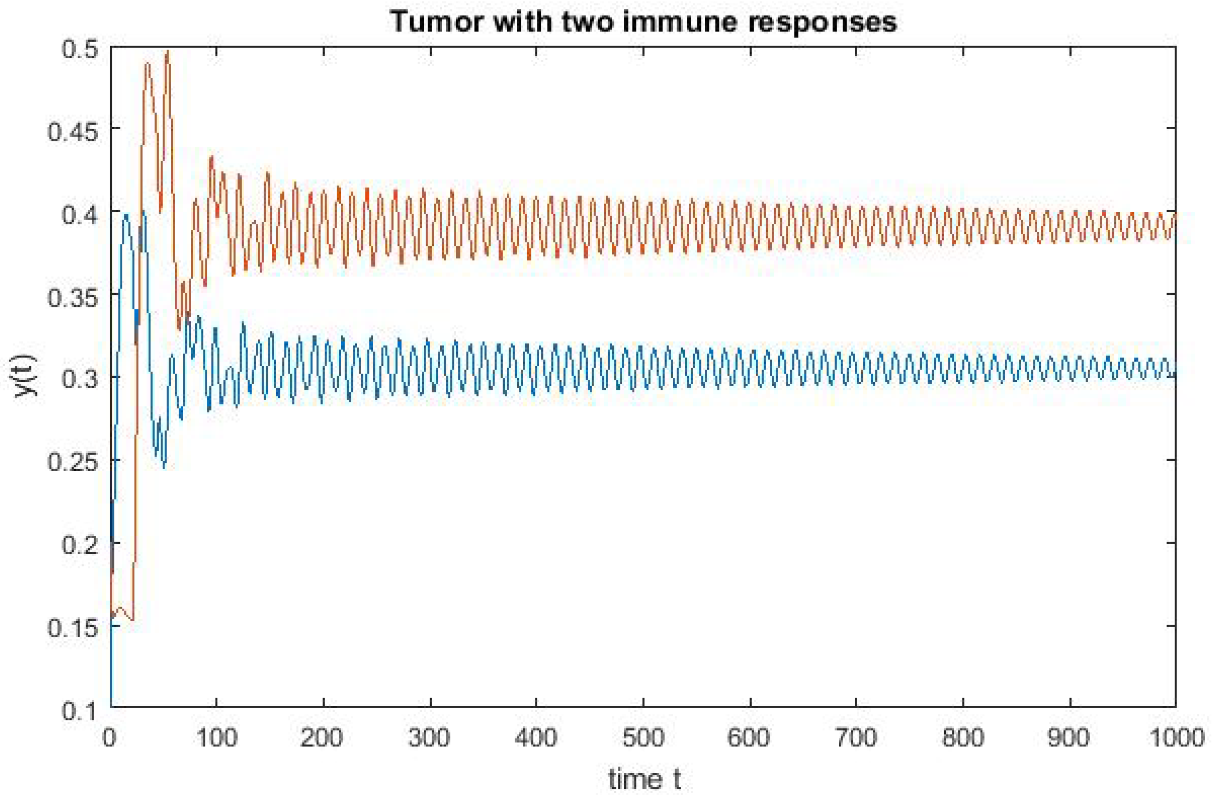
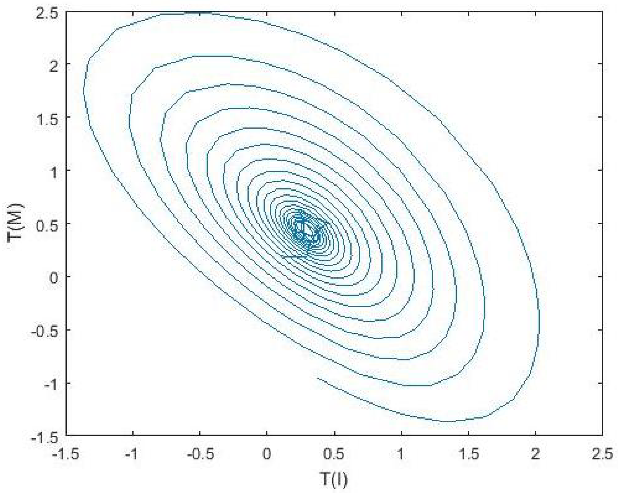
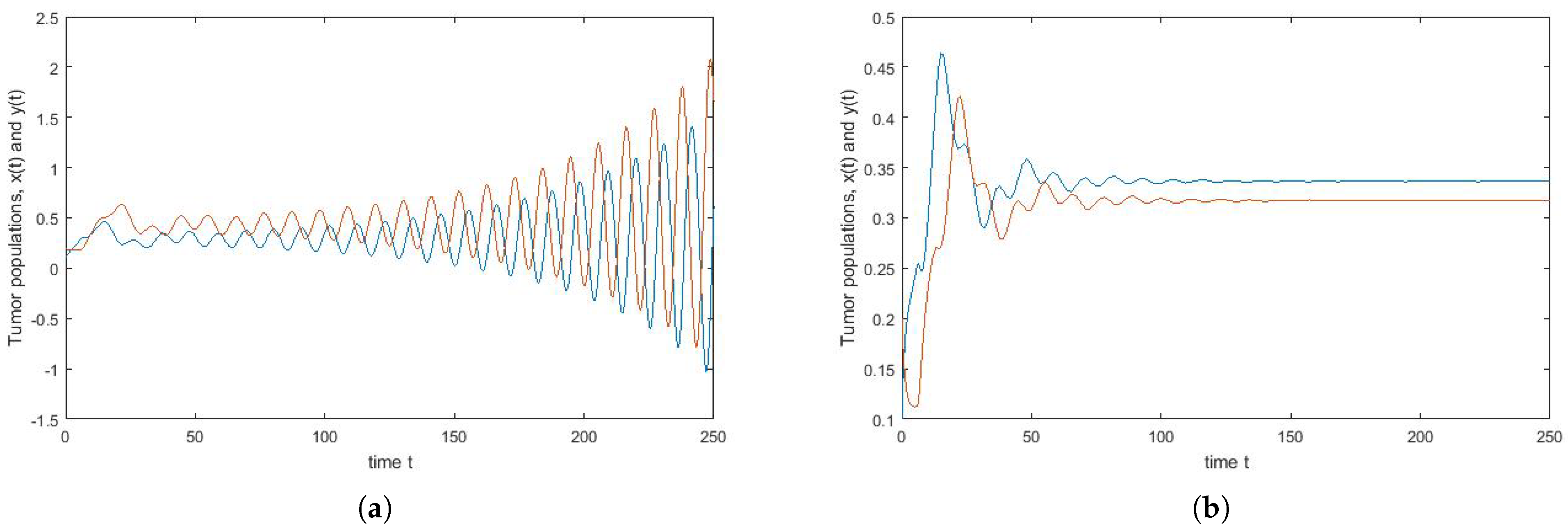
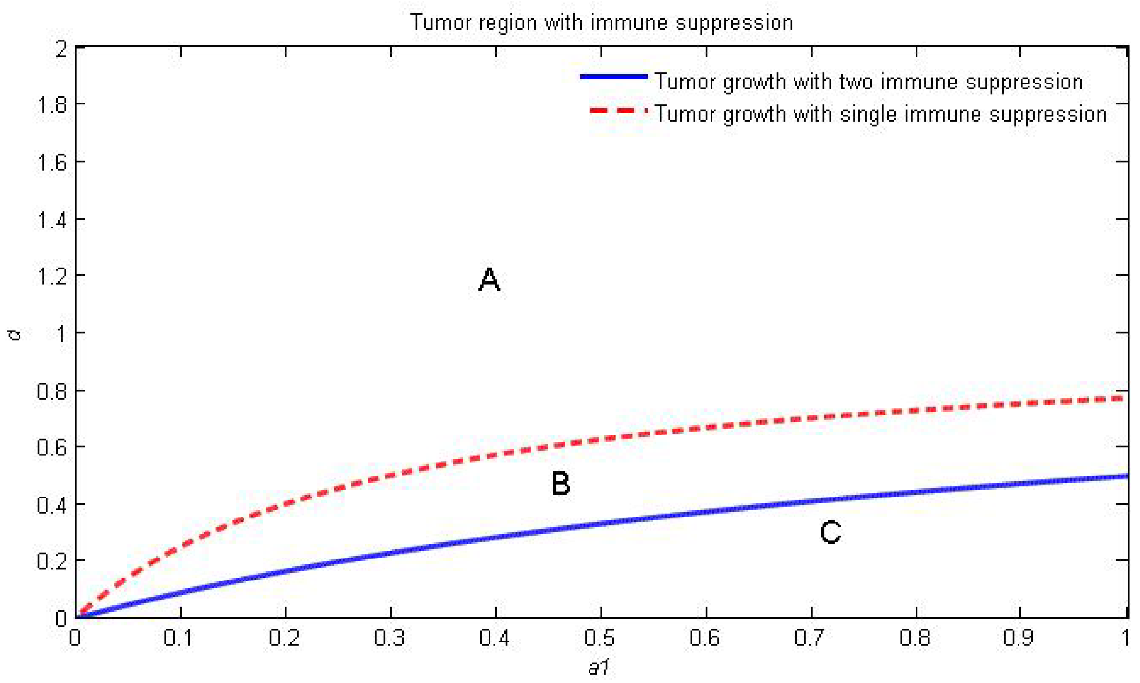
4. Numerical Simulation

The solutions presented in this section are calculated using dde23 function in Matlab version R2015a(8.5.0.197613) 64-bit (win64) 12 February 2015 [30]. DDE-Biftool, which is a Matlab package is used for numerical bifurcation analysis. Wolfram Mathematica version 11 is used to calculate the equilibrium points which must be solved numerically. Set parameters as $a_1=1$, $a_4=0.5$, $d_1=0.028$, $d_4=0.028$, $d_2=0$, $d_3=0$, $c_1=c_7=0.02$, $c_3=c_8=0.02$, $c_2=c_4=0.008$, $c_5=c_6=0.008$, $\alpha =\gamma =0.2$, $n=3$ and $r=1$. For these parameter values there are two fixed points, namely the tumour-free fixed point at $E_0=(0,0,15,0)$ and tumour fixed point with positive immune response at $E_1=(224.98,288.15,0.11,13.93)$. When $\tau =0$, the fixed point $E_0$ is stable as shown in the Figure 4, which means all the tumour population decays.

When $\tau >0$, conditions 1 and 2 in Theorem 1 are satisfied where it is showed that there is one positive root. Following from Equation (14), we have

$$S\left(\mu \right)={\mu }^2-0.82\mu -0.0319=0,$$

where ${\mu }_1=0.8572$ and ${\mu }_2=-0.372$. We are only interested in positive real roots. Since ${\omega }_0=\pm \sqrt{\mu }$, then we have ${\omega }_0=\pm \sqrt{0.852}=\pm 0.9259$. Using Equation (16), with the given parameter and corresponding ${\omega }_{\pm }$, we obtain the following critical time delay values as written in

Table 2. Values of ${\tau }_k^{+}$ and ${\tau }_k^{-}$ for $n=0,1,2,3,4$.

${\tau }_0^{+}$	1.69531 i	${\tau }_0^{-}$	−1.68244
${\tau }_1^{+}$	7.33207 + 1.69531 i	${\tau }_1^{-}$	5.64962
${\tau }_2^{+}$	14.6641 + 1.69531 i	${\tau }_2^{-}$	12.9817
${\tau }_3^{+}$	21.9962 + 1.69531 i	${\tau }_3^{-}$	20.3138
${\tau }_4^{+}$	29.3283 + 1.69531 i	${\tau }_4^{-}$	27.6458

.

Tumour populations is shown in Figure 5, Figure 6, Figure 7 and Figure 8 with different values of $\tau$. Now, consider the system at $E_1$. Since the conditions failed the stability conditions in Theorem 2, the system is said to be unstable for all tau.

Now, set parameter as $a_1=1$, $a_4=0.5$, $d_1=0.28$, $d_4=0.28$, $d_2=0$, $d_3=0$, $c_1=c_7=0.02$, $c_3=c_8=0.02$, $c_2=c_4=0.008$, $c_5=c_6=0.008$, $\alpha =\gamma =0.2$, $n=3$ and $r=1$. In this case there are two fixed points: $E_0=(0,0,1.5,0)$ and $E_1=(0.1,0.39,2.62,11.41)$. By computing the roots as given by Equation (14), it can see that $E_0$ is unstable for all values of delay. However, $E_1$ has stability switching where the stability of the fixed point switches from stable to unstable at some ${\tau }^{*}$. Again, at some ${\tau }^{*}$, the system switches from unstable to stable. Oscillations around this fixed point would therefore correspond to a tumour which grows and shrinks with no application of treatment. Figure 9 and Figure 10 were generated using MATLAB.

When $\tau >0$, conditions 1 and 2 in Theorem 1 are satisfied where it is shows that there is one positive root. Following from Equation (14), we have

$$S\left(\mu \right)={\mu }^2-0.9982\mu -0.02209=0,$$

where ${\mu }_1=1.1847$ and ${\mu }_2=-1.865$. We are only interested in positive real roots. Since ${\omega }_0=\pm \sqrt{\mu }$, then we have ${\omega }_0=\pm \sqrt{1.1847}=\pm 1.0884$. Using Equation (16), with the given parameter and corresponding ${\omega }_{\pm }$, we obtain critical time delay values as ${\tau }_1=5.99$, ${\tau }_2=8.5669$, ${\tau }_3=16.7676$ and ${\tau }_4=22.0586$. Time delay parameter, ${\tau }^{*}$ is shown in Figure 11.

Figure 12, Figure 13, Figure 14 and Figure 15 show the tumour populations at interphase and mitosis when the value of $\tau$ is varied. From the figures, we can see that the tumour decays as time increases, which means that the system slowly changes from an unstable state to a stable one. Figure 16 and Figure 17 show that bifurcation happens at each $\tau$ value.

Varying Rate at Which Tumour Cell Enter Mitosis, $a_1$

Mitosis is the phase where two daughter cells are produced from a single cell. A tumour cell from interphase that completes the process will enter mitosis to complete the cycle. The tumour cell can be controlled from dividing if we can control the number of cells that enter mitosis. If the number of cells that enter mitosis decrease, then we can reduce the number of tumour cells produced. The effects of proliferation rate, $a_1$, are varied in order to see the changes of the tumour populations in interphase and mitosis. We choose $a_1$ as 1.2 and 0.7, respectively. If the value of $a_1=1.2$, the system oscillates and becomes unstable since a high proliferation rate can tolerate more tumour cells in the system, resulting in tumour growth as in Figure 18. However, the system is stable when the rate of proliferation is decreased, $a_1=0.7$ as in Figure 19.

5. Discussion and Conclusions

This paper presents a model of the interaction between tumour population and immune responses. It is based on Villasana’s model [24] by extending it to include another immune response, which is NK cells. Tumour populations are split into two phases related to the cell cycle, interphase and M phase (mitosis). Time delay, $\tau$, is added in the model to describe the length of the interphase. Immune cells are assumed to interact with the cell in all the stages. The model describes how NK cells and CD$8^{+}$ T cell affect the growth of the tumour cell populations at interphase and mitosis.

The immune system is a system that reacts directly to fight when it detects an abnormal cell (tumour cell). By adding immune responses in the model, it greatly helps to stabilise the system and inhibit further growth of tumour cells. The combined effect of the NK and CD$8^{+}$ T cells can eliminate larger tumour cell compared to the individual effect of the immune cell. This is shown when the stability of the system is tested. Based on condition in (5), we can see that tumour growth mainly depends on the death rate of the cells and reproduction rate in the absence of the immune system. Tumours begin to grow if the reproduction rate is greater than the death rate of tumour cells in the mitosis. In that case, without the immune system, the tumour will grow. By adding the NK CD$8^{+}$ T cell in the model, we show that they greatly help to inhibit the growth of the tumour. Figure 20 shows the tumour region involving one immune suppression (Region B and C) and two immune suppression (Region C). Regions B and C represent the tumour growth while the tumour decay is represented by Region A. The region of tumour growth with double immune suppression is smaller than the case with single immune suppression as in [24].

The involving of immune responses (NK cell and CD$8^{+}$ T cell) has helped the system to stay stable. However, at a certain stage the tumour will grow when both immune cells lose their ability to fight the tumour cells. However, NK cell and CD$8^{+}$ T cell will lower the chance of tumour cells reaching maturity. Each of the immune cells have their own role in fighting the tumour cells. The NK cell can recognise and directly attack the tumour cells before they replicate and grow. Compared to this, CD$8^{+}$ T cell needs to obtain the signal and will react to the tumour cell after getting the signal. CD$8^{+}$ T cell needs some times to recognise the tumour cells before attacking them. Furthermore, the NK cell plays an important role in the activation of the immune system since its can activate specific immune response CD$8^{+}$ T cell (which is the interaction between the tumour cell and NK cell).

The presented model is simple, but it gives further information about the dynamics of the system. The inclusion of another immune response gives us a deep insight into the tumour growth and helps us understand how the interactions between them contribute to lyse tumour cells. However, this model is general and not intended to fit every type of tumour growth, since each tumour cell type presents different difficulties.

References

1. de Martel, C.; Georges, D.; Bray, F.; Ferlay, J.; Clifford, G.M. Global burden of cancer attributable to infections in 2018: A worldwide incidence analysis. Lancet Glob. Health 2020, 8, e180–e190. [Google Scholar] [CrossRef] [Green Version]
2. Sung, H.; Ferlay, J.; Siegel, R.L.; Laversanne, M.; Soerjomataram, I.; Jemal, A.; Bray, F. Global cancer statistics 2020: GLOBOCAN estimates of incidence and mortality worldwide for 36 cancers in 185 countries. CA Cancer J. Clin. 2021, 71, 209–249. [Google Scholar] [CrossRef] [PubMed]
3. Eftimie, R.; Bramson, J.L.; Earn, D.J. Interactions between the immune system and cancer: A brief review of non-spatial mathematical models. Bull. Math. Biol. 2011, 73, 2–32. [Google Scholar] [CrossRef] [PubMed]
4. de Pillis, L.G.; Gu, W.; Radunskaya, A.E. Mixed immunotherapy and chemotherapy of tumors: Modeling, applications and biological interpretations. J. Theor. Biol. 2006, 238, 841–862. [Google Scholar] [CrossRef] [PubMed]
5. d’Onofrio, A. A general framework for modeling tumor-immune system competition and immunotherapy: Mathematical analysis and biomedical inferences. Phys. D Nonlinear Phenom. 2005, 208, 220–235. [Google Scholar] [CrossRef] [Green Version]
6. d’Onofrio, A. Metamodeling tumor–immune system interaction, tumor evasion and immunotherapy. Math. Comput. Model. 2008, 47, 614–637. [Google Scholar] [CrossRef]
7. Burnet, F. Immunological aspects of malignant disease. Lancet 1967, 289, 1171–1174. [Google Scholar] [CrossRef]
8. Kirschner, D.; Panetta, J.C. Modeling immunotherapy of the tumor–immune interaction. J. Math. Biol. 1998, 37, 235–252. [Google Scholar] [CrossRef] [Green Version]
9. Kirkwood, J.M.; Butterfield, L.H.; Tarhini, A.A.; Zarour, H.; Kalinski, P.; Ferrone, S. Immunotherapy of cancer in 2012. CA Cancer J. Clin. 2012, 62, 309–335. [Google Scholar] [CrossRef]
10. Esfahani, K.; Roudaia, L.; Buhlaiga, N.A.; Del Rincon, S.; Papneja, N.; Miller, W. A review of cancer immunotherapy: From the past, to the present, to the future. Curr. Oncol. 2020, 27, 87–97. [Google Scholar] [CrossRef]
11. Fruci, D.; Lo, M.E.; Cifaldi, L.; Locatelli, F.; Tremante, E.; Benevolo, M.; Giacomini, P. T and NK cells: Two sides of tumor immunoevasion. J. Transl. Med. 2013, 11, 30. [Google Scholar] [CrossRef] [PubMed] [Green Version]
12. Gajewski, T.F.; Schreiber, H.; Fu, Y.X. Innate and adaptive immune cells in the tumor microenvironment. Nat. Immunol. 2013, 14, 1014–1022. [Google Scholar] [CrossRef] [PubMed] [Green Version]
13. Lee, S.W.; Park, H.J.; Kim, N.; Hong, S. Natural Killer Dendritic Cells Enhance Immune Responses Elicited by α-Galactosylceramide-Stimulated Natural Killer T Cells. BioMed Res. Int. 2013, 2013, 460706. [Google Scholar] [CrossRef] [Green Version]
14. Levy, E.M.; Roberti, M.P.; Mordoh, J. Natural killer cells in human cancer: From biological functions to clinical applications. BioMed Res. Int. 2011, 2011, 676198. [Google Scholar] [CrossRef] [PubMed]
15. de Pillis, L.G.; Radunskaya, A.E.; Wiseman, C.L. A validated mathematical model of cell-mediated immune response to tumor growth. Cancer Res. 2005, 65, 7950–7958. [Google Scholar] [CrossRef] [Green Version]
16. Admon, M.R.; Maan, N. Modelling tumor growth with immune response and drug using ordinary differential equations. J. Teknologi 2017, 79, 49–59. [Google Scholar] [CrossRef] [Green Version]
17. Awang, N.A.; Maan, N. Analysis of tumor populations and immune system interaction model. In Proceedings of the 23rd Malaysian National Symposium of Mathematical Sciences (SKSM23), Johor, Malaysia, 27–29 September 2016; Volume 1750, p. 030049. [Google Scholar]
18. Admon, M.R.; Maan, N. Modelling of macrophage interactions in breast cancer by partial differential equations. Malays. J. Fundam. Appl. Sci. 2017, 13, 113–117. [Google Scholar]
19. Abdulkareem, A.I.; Jemon, K.; Maan, N. Stability and Sensitivity Analysis of Tumor-induce immune Suppression with Time Delay. J. Adv. Res. Dyn. Control. Syst. 2020, 12, 1321–1331. [Google Scholar]
20. de Pillis, L.; Radunskaya, A. A mathematical model of immune response to tumor invasion. In Computational Fluid and Solid Mechanics 2003; Elsevier Science Ltd.: Oxford, UK, 2003; pp. 1661–1668. [Google Scholar]
21. Pang, L.; Liu, S.; Zhang, X.; Tian, T. Mathematical modeling and dynamic analysis of anti-tumor immune response. J. Appl. Math. Comput. 2020, 62, 473–488. [Google Scholar] [CrossRef]
22. Kuznetsov, V.A.; Makalkin, I.A.; Taylor, M.A.; Perelson, A.S. Nonlinear dynamics of immunogenic tumors: Parameter estimation and global bifurcation analysis. Bull. Math. Biol. 1994, 56, 295–321. [Google Scholar] [CrossRef]
23. de Pillis, L.; Renee Fister, K.; Gu, W.; Collins, C.; Daub, M.; Gross, D.; Moore, J.; Preskill, B. Mathematical model creation for cancer chemo-immunotherapy. Comput. Math. Methods Med. 2009, 10, 165–184. [Google Scholar] [CrossRef] [Green Version]
24. Villasana, M.; Radunskaya, A. A delay differential equation model for tumor growth. J. Math. Biol. 2003, 47, 270–294. [Google Scholar] [CrossRef] [PubMed]
25. Liu, W.; Hillen, T.; Freedman, H. A mathematical model for M-phase specific chemotherapy including the G0-phase and immunoresponse. Math. Biosci. Eng. 2007, 4, 239. [Google Scholar] [PubMed]
26. Lodish, H.F.; Berk, A.; Kaiser, C.A.; Kaiser, C.; Krieger, M.; Scott, M.P.; Matsudaira, P. Molecular Cell Biology; Macmillan: New York, NY, USA, 2000; Volume 4. [Google Scholar]
27. Kastan, M.B.; Bartek, J. Cell-cycle checkpoints and cancer. Nature 2004, 432, 316–323. [Google Scholar] [CrossRef]
28. de Villegas, M.V. A Delay Differential Equation Model for Tumor Growth. Ph.D. Thesis, Claremont University, Claremont, CA, USA, 2001. [Google Scholar]
29. Mahasa, K.J.; Ouifki, R.; Eladdadi, A.; de Pillis, L. Mathematical model of tumor–immune surveillance. J. Theor. Biol. 2016, 404, 312–330. [Google Scholar] [CrossRef] [Green Version]
30. Matlab. Version 8.5.0.197613 (R2015a); The MathWorks Inc.: Natick, MA, USA, 2015. [Google Scholar]
Figure 1. Flow chart of Tumour-NK and CD8 + T cells interaction model.
Mathematics 10 02193 g001
Figure 2. Stability map around the tumour-free equilibrium point, E 0 when τ > 0 .
Mathematics 10 02193 g002
Figure 3. Stability map around the tumour-free equilibrium point, E 0 when τ = 0 .
Mathematics 10 02193 g003
Figure 4. Tumour population with two immune response in the absence of delay at the fixed point E 0 = ( 0 , 0 , 15 , 0 ) .
Mathematics 10 02193 g004
Figure 5. Tumour population with two immune response when τ = 5.6496 at E 0 = ( 0 , 0 , 15 , 0 ) .
Mathematics 10 02193 g005
Figure 6. Tumour population with two immune response when τ = 12.9817 at E 0 = ( 0 , 0 , 15 , 0 ) .
Mathematics 10 02193 g006
Figure 7. Tumour population with two immune response when τ = 20.3138 at E 0 = ( 0 , 0 , 15 , 0 ) .
Mathematics 10 02193 g007
Figure 8. Tumour population with two immune response when τ = 27.6458 at E 0 = ( 0 , 0 , 15 , 0 ) .
Mathematics 10 02193 g008
Figure 9. Tumour population with two immune response when τ = 0 at E 1 = ( 0.1 , 0.39 , 2.62 , 11.41 ) .
Mathematics 10 02193 g009
Figure 10. Tumour populations at interphase (blue line) and mitosis (red line) when τ = 0 at E 1 = ( 0.1 , 0.39 , 2.62 , 11.41 ) .
Mathematics 10 02193 g010
Figure 11. Time delay parameter, τ * at E 1 = ( 0.1 , 0.39 , 2.62 , 11.41 ) . Green line represents stable and red line represents unstable, respectively.
Mathematics 10 02193 g011
Figure 12. Simulation result of tumour populations at interphase (blue line) and mitosis (red line) when τ = 5.99 for the system (1) at E 1 = ( 0.1 , 0.39 , 2.62 , 11.41 ) .
Mathematics 10 02193 g012
Figure 13. Simulation result of tumour populations at interphase (blue line) and mitosis (red line) when τ = 8.5669 for the system (1) at E 1 = ( 0.1 , 0.39 , 2.62 , 11.41 ) .
Mathematics 10 02193 g013
Figure 14. Simulation result of tumour populations at interphase (blue line) and mitosis (red line) when τ = 16.7676 for the system (1) at E 1 = ( 0.1 , 0.39 , 2.62 , 11.41 ) .
Mathematics 10 02193 g014
Figure 15. Simulation result of tumour populations at interphase (blue line) and mitosis (red line) when τ = 22.0586 for the system (1) at E 1 = ( 0.1 , 0.39 , 2.62 , 11.41 ) .
Mathematics 10 02193 g015
Figure 16. Periodic solutions from Hopf bifurcation (∗) at different values of τ for the system (1), (a) τ = 5.99 ; and (b) τ = 8.5669 ; at E 1 = ( 0.1 , 0.39 , 2.62 , 11.41 ) . Stability switching occurred from stable (green line) to unstable (red line) and vice versa.
Mathematics 10 02193 g016
Figure 17. Periodic solutions from Hopf bifurcation (∗) at different values of τ for the system (1), (a) τ = 16.7676 ; and (b) τ = 22.0586 ; at E 1 = ( 0.1 , 0.39 , 2.62 , 11.41 ) . Stability switching occurred from stable (green line) to unstable (red line) and vice versa.
Mathematics 10 02193 g017
Figure 18. Unstable limit cycle of tumour populations when a 1 = 1.2 at τ = 5.99 .
Mathematics 10 02193 g018
Figure 19. Simulation results of tumour populations (interphase, x ( t ) and mitosis, y ( t ) ) when τ = 5.99 . (a) a 1 = 1.2 ; (b) a 1 = 0.7 .
Mathematics 10 02193 g019
Figure 20. Regions of the stability of a 1 and d are obtained. d represents the total cell loss at mitosis. Region A represents tumour decay and Region B and C represent tumour growth. When two immune suppressions are added, the curve lies consistently below the curve with single immune suppression.
Mathematics 10 02193 g020