
Hybridization of Manta-Ray Foraging Optimization Algorithm with Pseudo Parameter-Based Genetic Algorithm for Dealing Optimization Problems and Unit Commitment Problem


Abstract
:1. Introduction
- The manta-ray foraging optimization (MRFO) technique is proposed to be combined with a pseudo-parameter-based genetic algorithm (GA) to overcome and improve the poor performance of standard MRFO.
- The GA’s objective function depends only on three variables, whatever the number of independent variables in the problem. The dimension of the optimization problem will not affect the number of the GA’s variables leading to less computational burden.
- The suggested approach uses GA to take out the manta-ray algorithm from any local minimum to a better local minimum until an optimal solution is found.
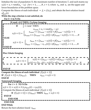
2. MRFO Overview
| Algorithm 1. Pseudo-code of MRFO algorithm. |
 |
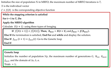
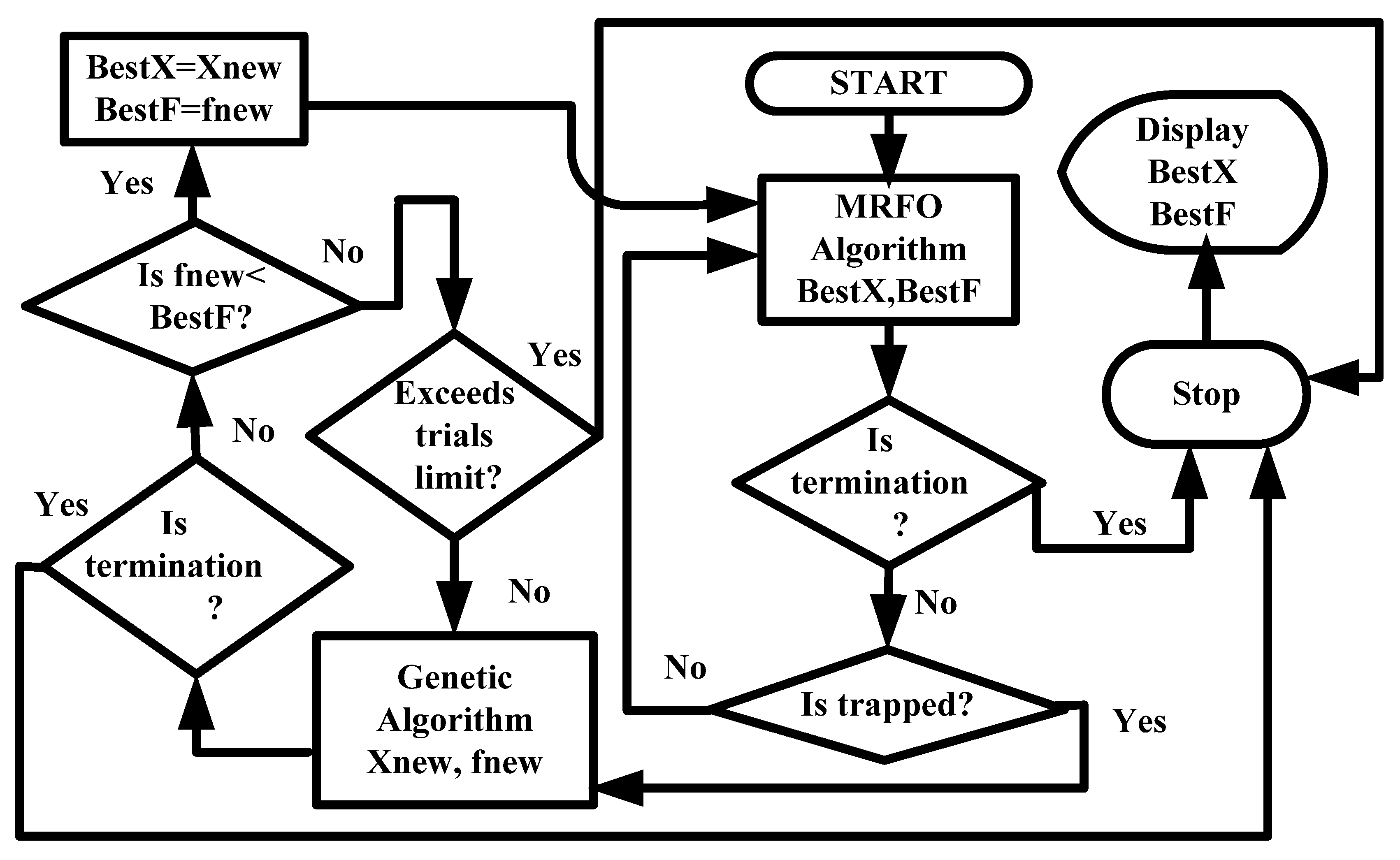
3. The Proposed Algorithm (PGA-MRFO)
3.1. Flow Chart and General Description of the Algorithm
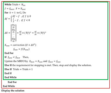
3.2. Mathematical Formulation of the Genetic Objective Function
3.3. Detailed Steps of the Proposed Algorithm (PGA-MRFO)
- (a)
- It may satisfy the problem’s termination (stopping) criterion. Then, it will be approved as the optimum solution, and the search process will be terminated.
- (b)
- If it is better than the trapped solution of MRFO, it will replace the MRFO’s trapping solution, and the MRFO algorithm is reapplied.
- (c)
- Suppose the resulting solution is not better than the trapped solution of MRFO. In that case, it will be entered again into the GA to be improved according to the genetic objective function (step 2).
| Algorithm 2. Pseudo-code of PGA-MRFO. |
  |
4. Testing Performance of PGA-MRFO Algorithm
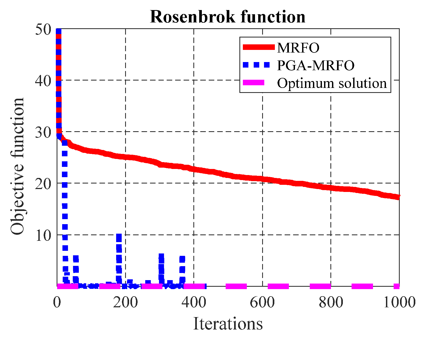
- For F5 (Figure 2), the PGA-MRFO algorithm converges to the optimum solution in 438 iterations. But the MRFO algorithm consumed 1000 iterations and could not reach the optimum solution.
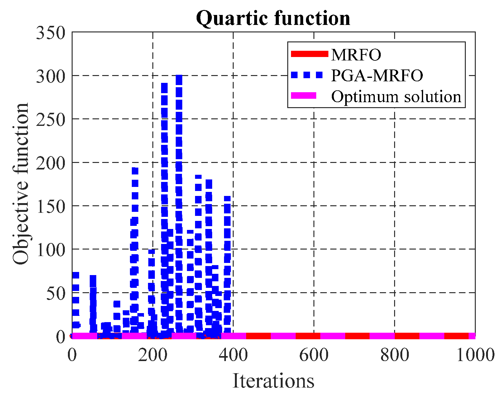
- For F7 (Figure 3), the PGA-MRFO algorithm converges to the optimum solution in fewer iterations than the MRFO algorithm.
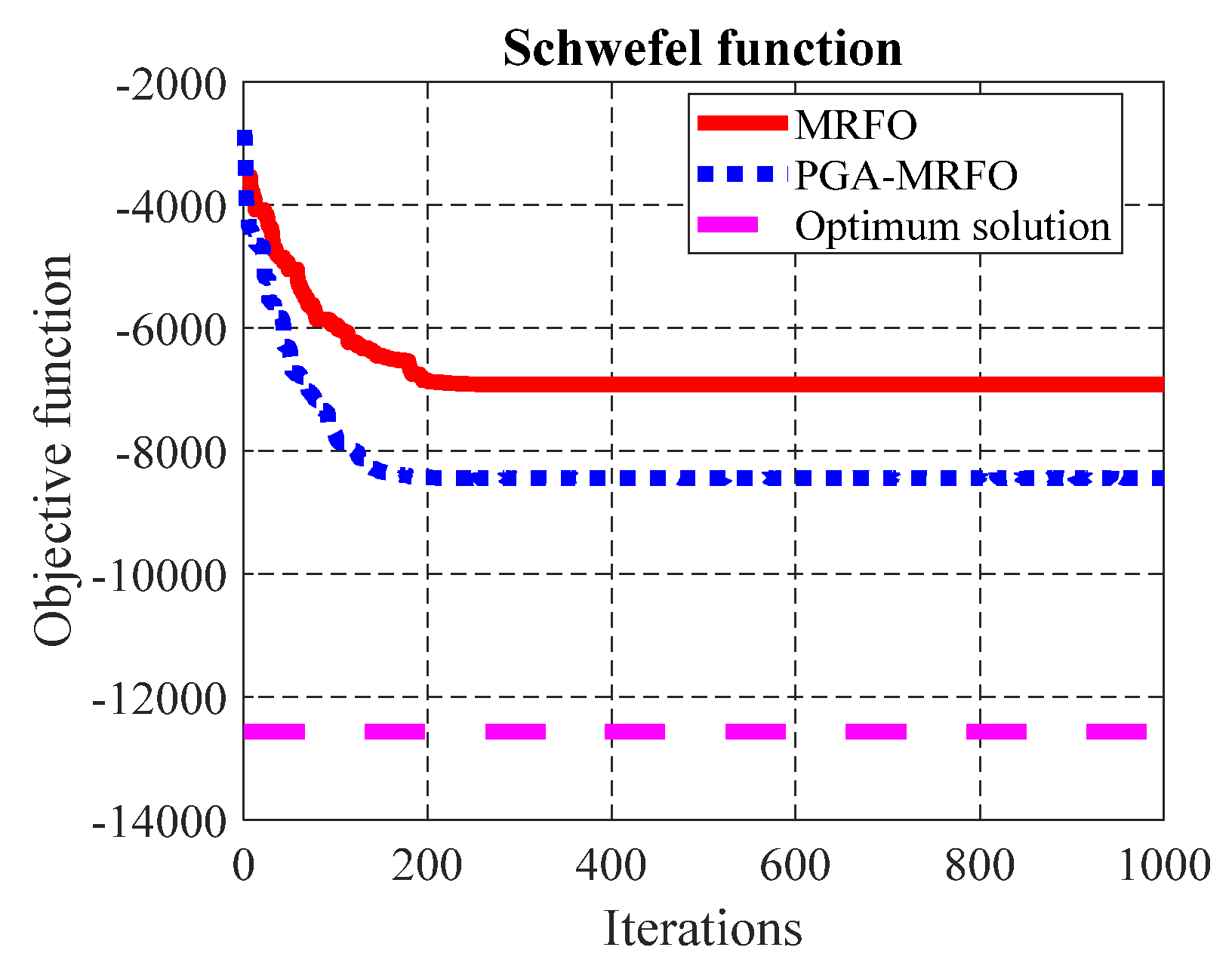
- For F8 (Figure 4), both algorithms failed to reach the optimum solution during 1000 iterations. However, PGA-MRFO converged to a better solution than the MRFO algorithm in the same number of iterations.
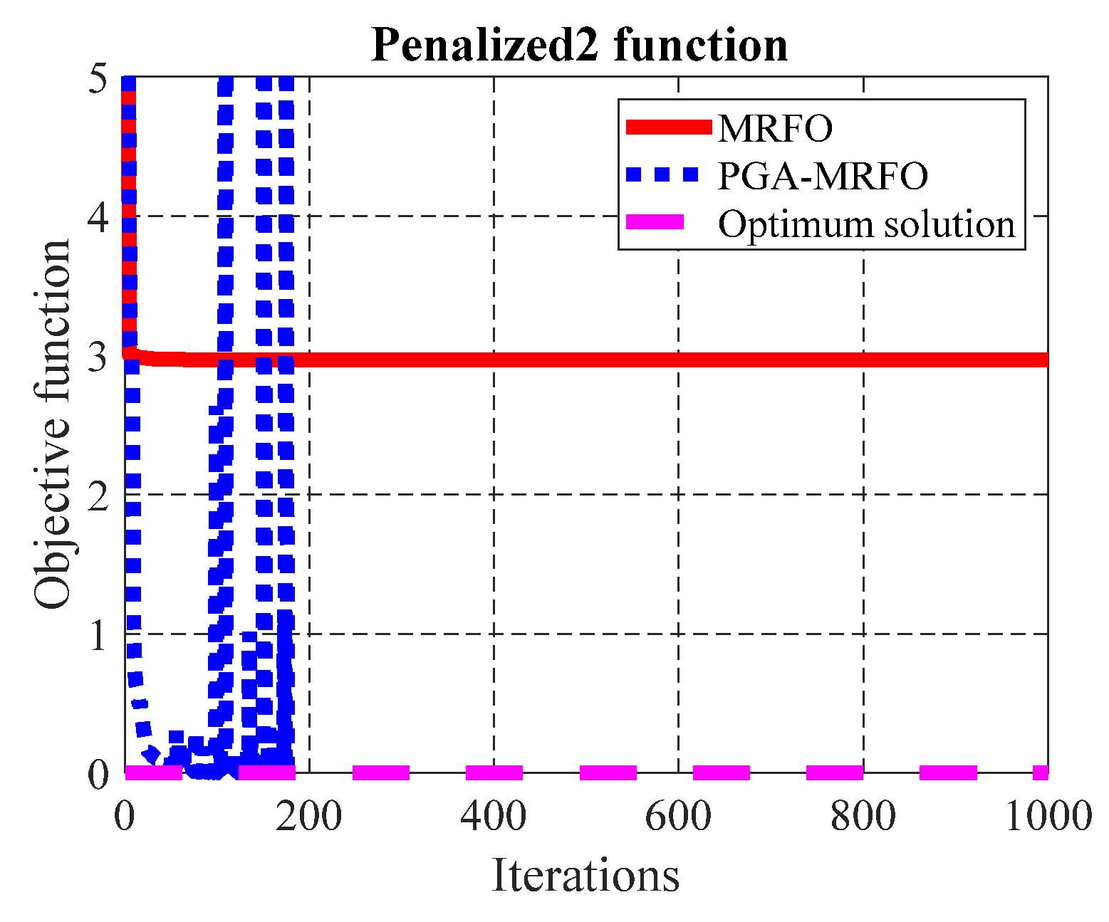
- For F13 (Figure 5), the PGA-MRFO algorithm reached the optimum solution using 181 iterations. The MRFO algorithm consumed 1000 iterations and failed to converge to the optimum solution.
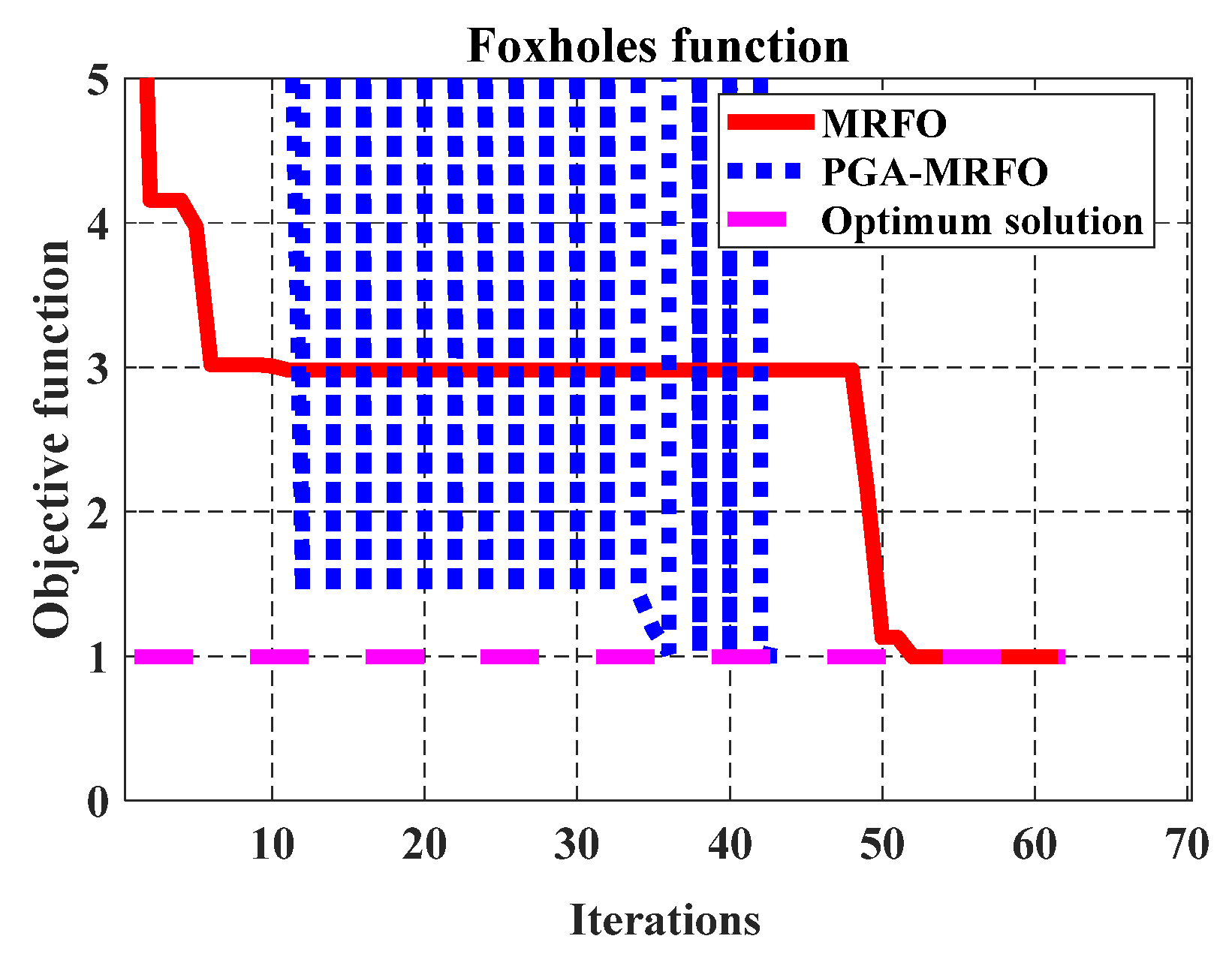
- For F14 (Figure 6), the PGA-MRFO reached the optimum solution in fewer iterations than the MRFO algorithm. It should be noticed that the fluctuations in the results using the PGA-MRFO algorithm represent the trials of the algorithm to get out of the local minimum and move to a better solution.
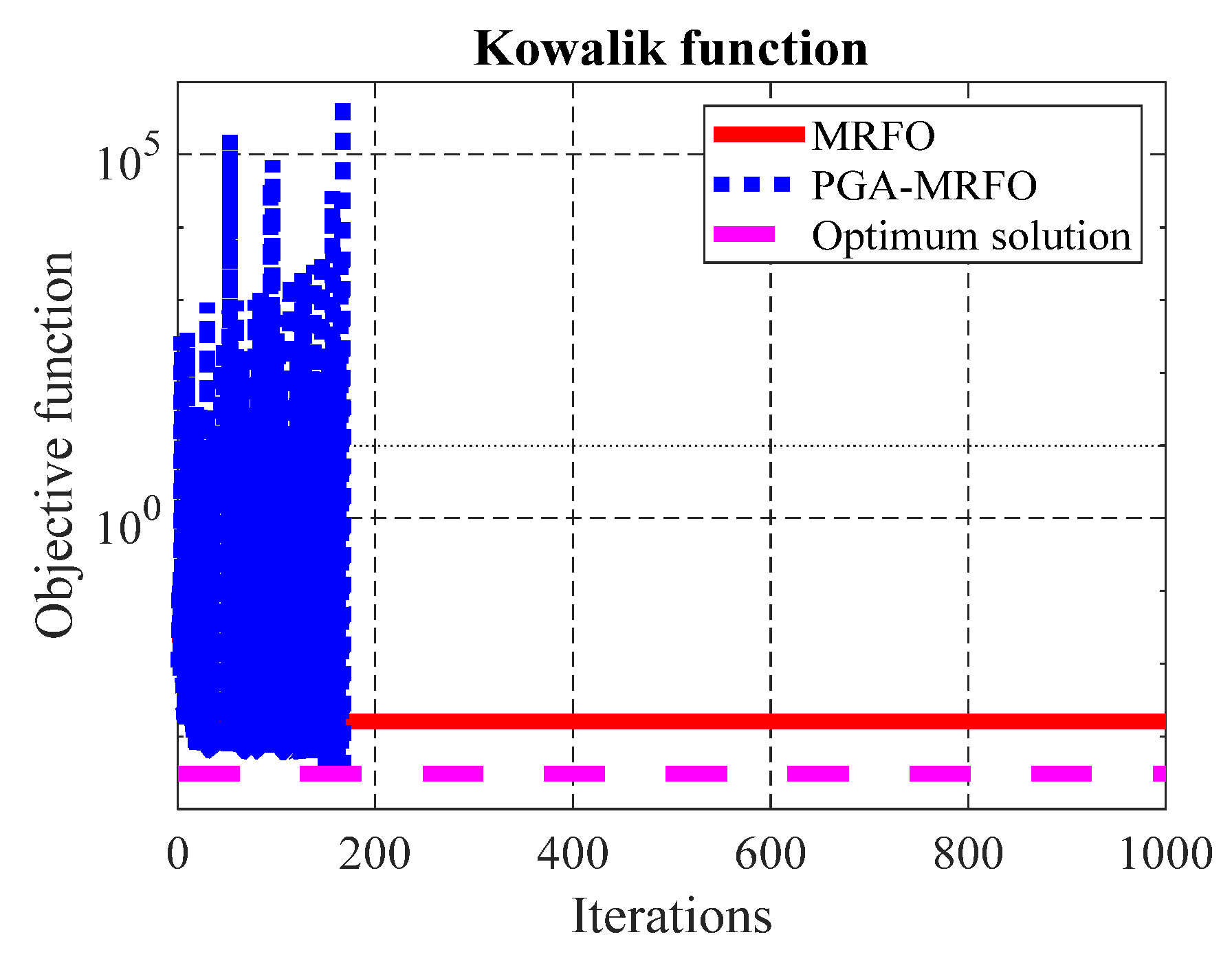
- For F15 (Figure 7), the PGA-MRFO reached the optimum solution in 169 iterations, while the MRFO algorithm could not get a near-optimal solution even after using 1000 iterations.
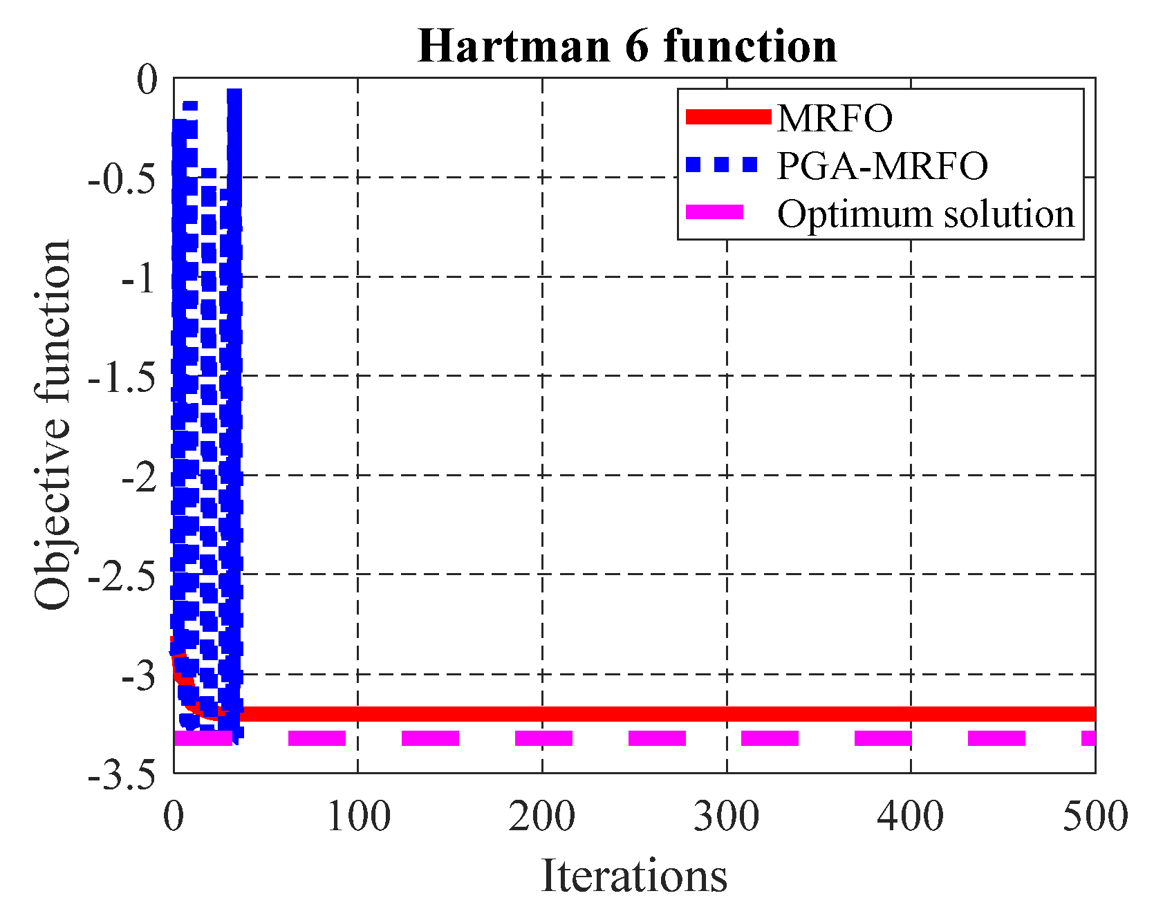
- For F20 (Figure 8), the PGA-MRFO algorithm converges to the optimum solution in 35 iterations. But, the MRFO algorithm spent 500 iterations and could not reach the optimum solution due to trapping in the local minimum.
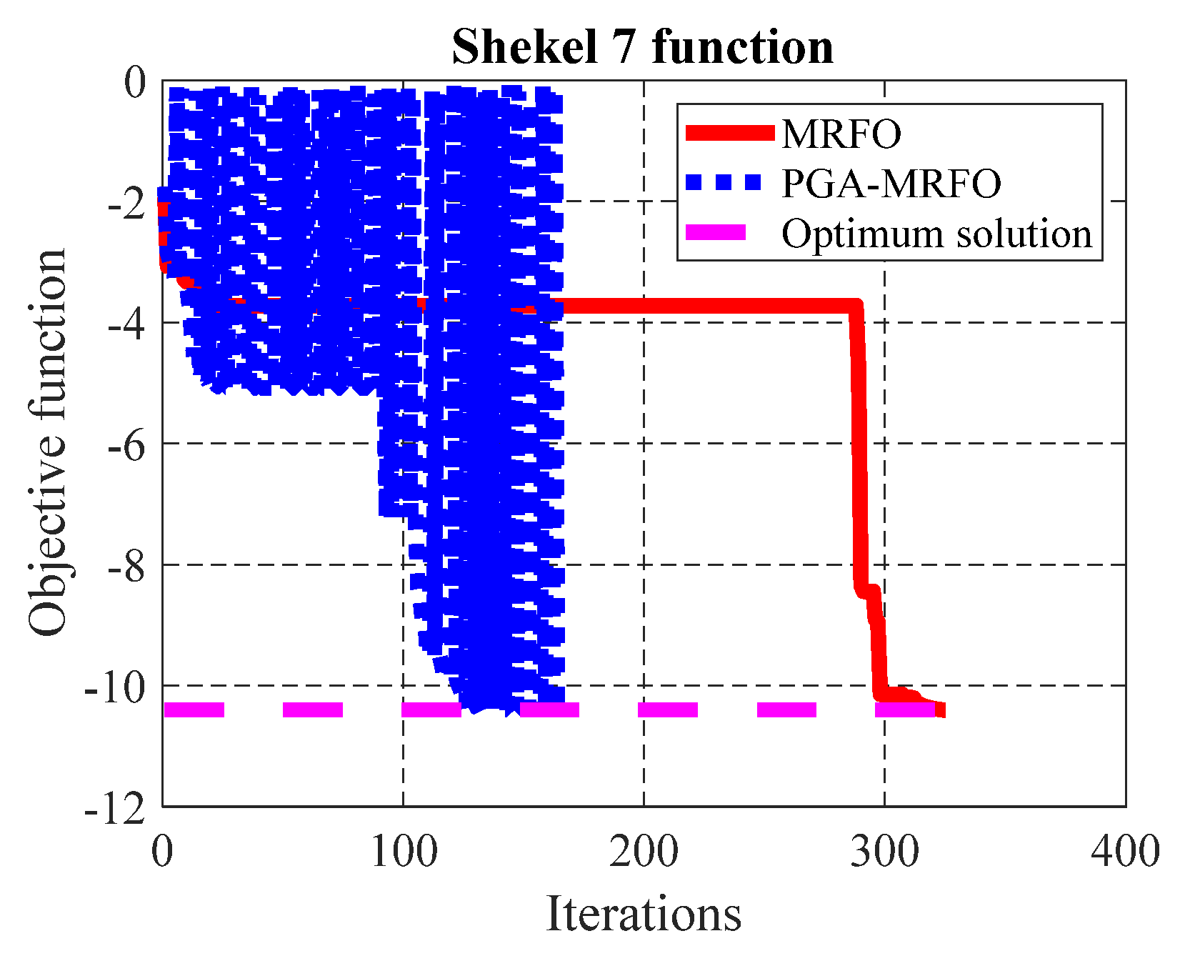
- For F21 (Figure 9), the PGA-MRFO algorithm got the optimum solution in 109 iterations. The MRFO algorithm consumed 1000 iterations without converging to the optimum solution due to falling into the local minimum.
- For F22 (Figure 10), the PGA-MRFO algorithm got the optimum solution in 169 iterations. But, the MRFO algorithm needed 325 iterations to reach the optimum solution, where this number of additional iterations was wasted in trapping into the local minimum.
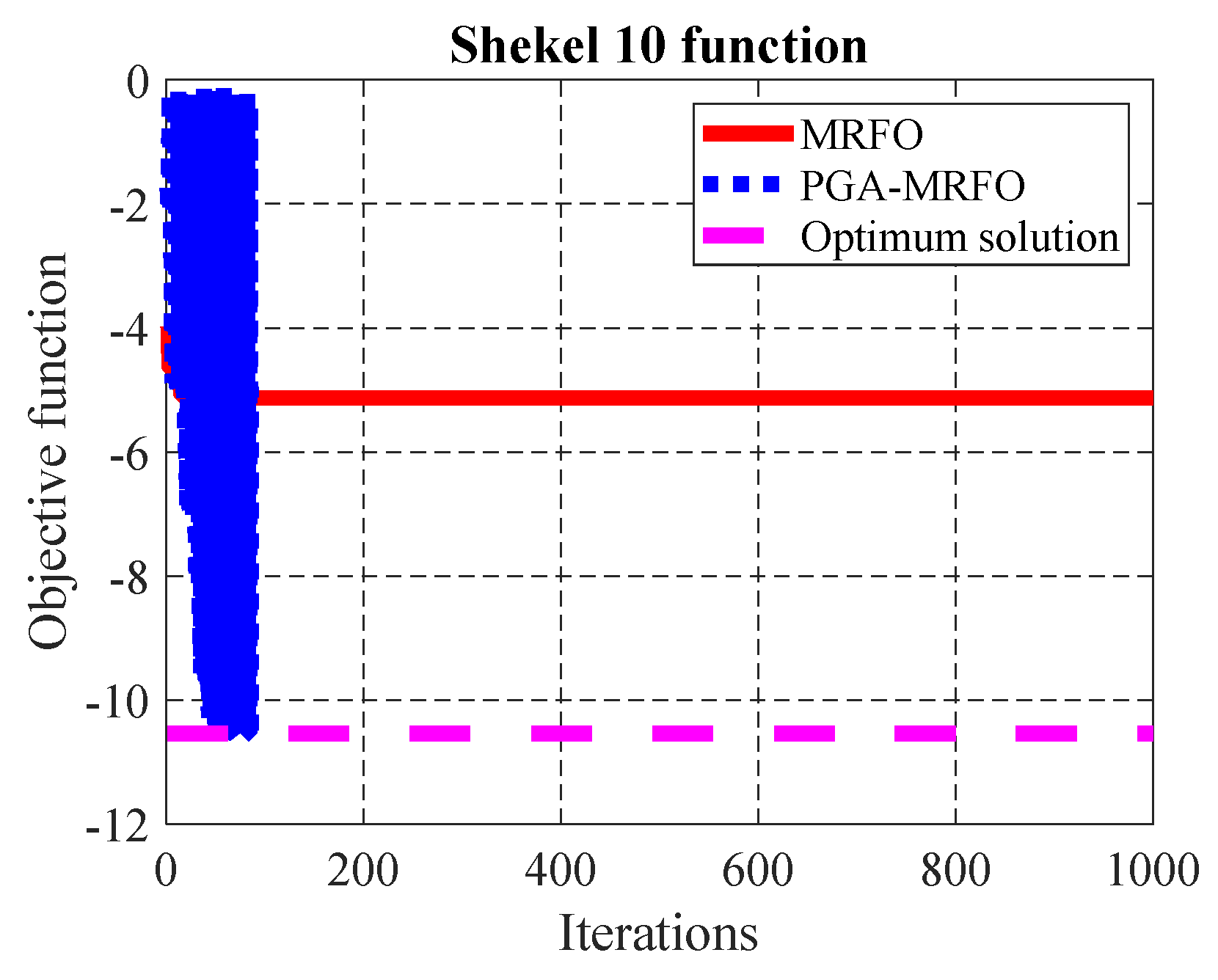
- For F23 (Figure 11), the PGA-MRFO algorithm got the optimum solution in 87 iterations. In contrast, the MRFO algorithm spent 1000 iterations and could not converge to the optimum solution. The figure shows that the MRFO algorithm consumed more than 800 iterations with almost the same solution due to trapping into the local minimum. But, the PGA-MRFO algorithm fluctuated until getting out of the local minimum and reached the optimum solution.
5. Application of PGA-MRFO Algorithm to Unit Commitment Problem
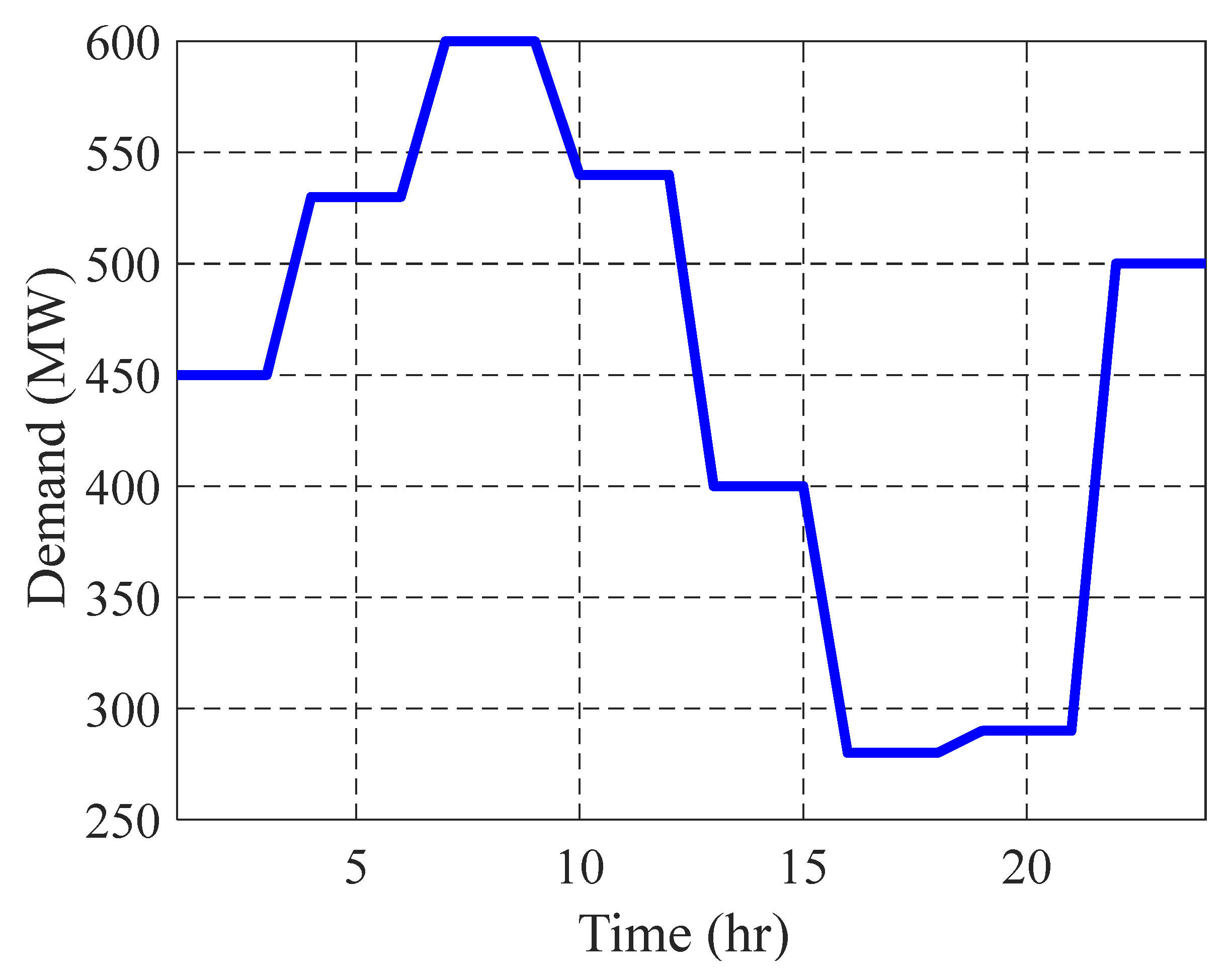
5.1. Description of the Problem
5.2. Problem Formulation
- Power balance constraint:
- 2.
- Generation limits:
- 3.
- Minimum up time:
- 4.
- Spinning reserve:
5.3. Test System Cases
5.3.1. Case 1: Four Units Test Power System
5.3.2. Case 2: Ten Units Test Power System
5.4. Modify the PGA-MRFO to Solve UC Problem
- Let be the best individual that is stuck in a local minimum.
- The limits of change in each variable [] can be calculated as:
- Each variable’s available set of discrete values represents the integer values between the lower and upper limits according to the span values calculated in step 1.
- 4.
- The two parameters in the GA are used to calculate the index of the proposed change in each variable. This index is approximated as:
- 5.
- After identifying the index, the new individual-based genetic parameters will be defined as:
- 6.
- For each individual in the genetic population, the new solution is calculated according to these five steps. Then, its objective function is calculated according to Equation (29), and the corresponding fitness function of the GA is calculated according to Equation (30).
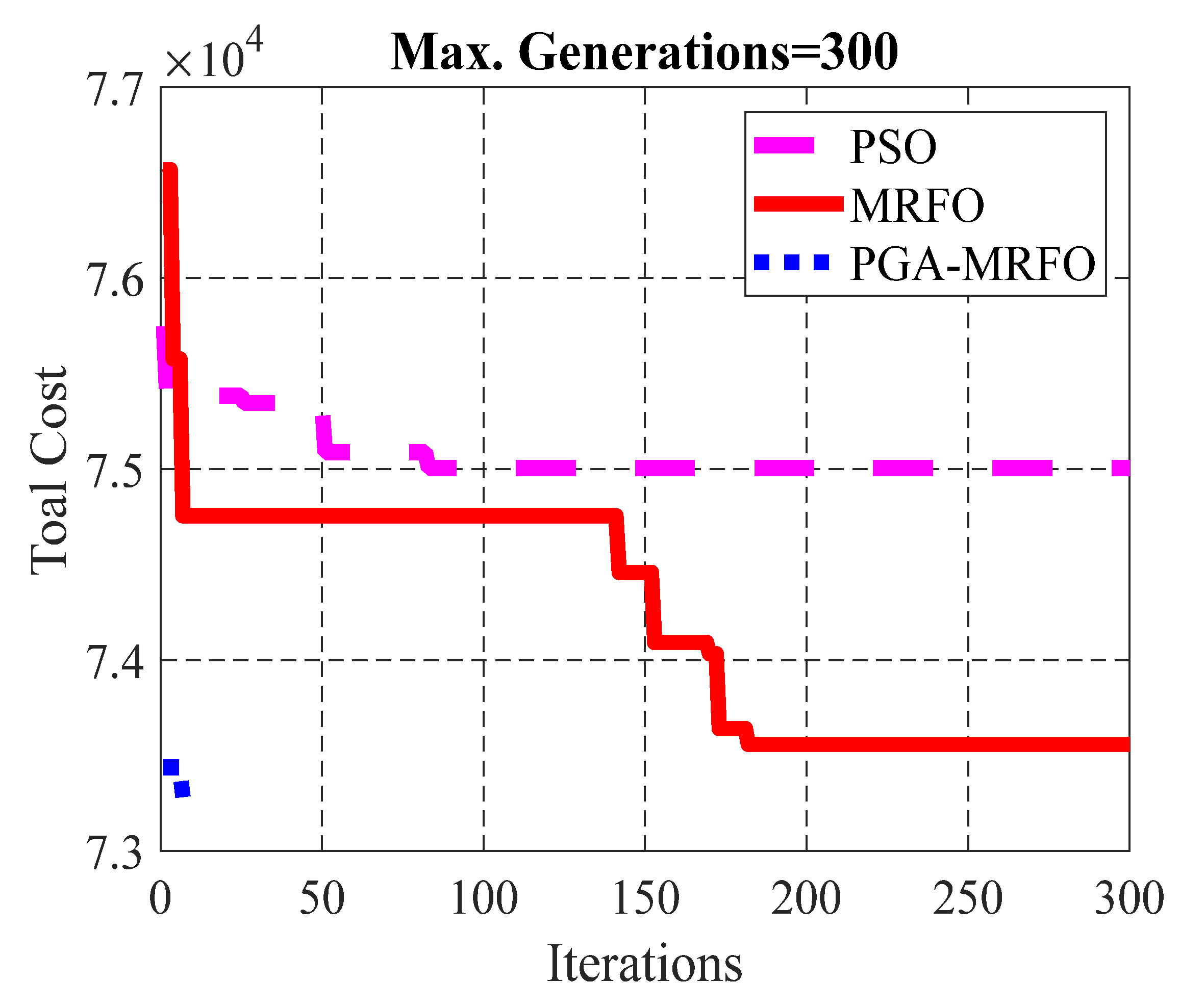
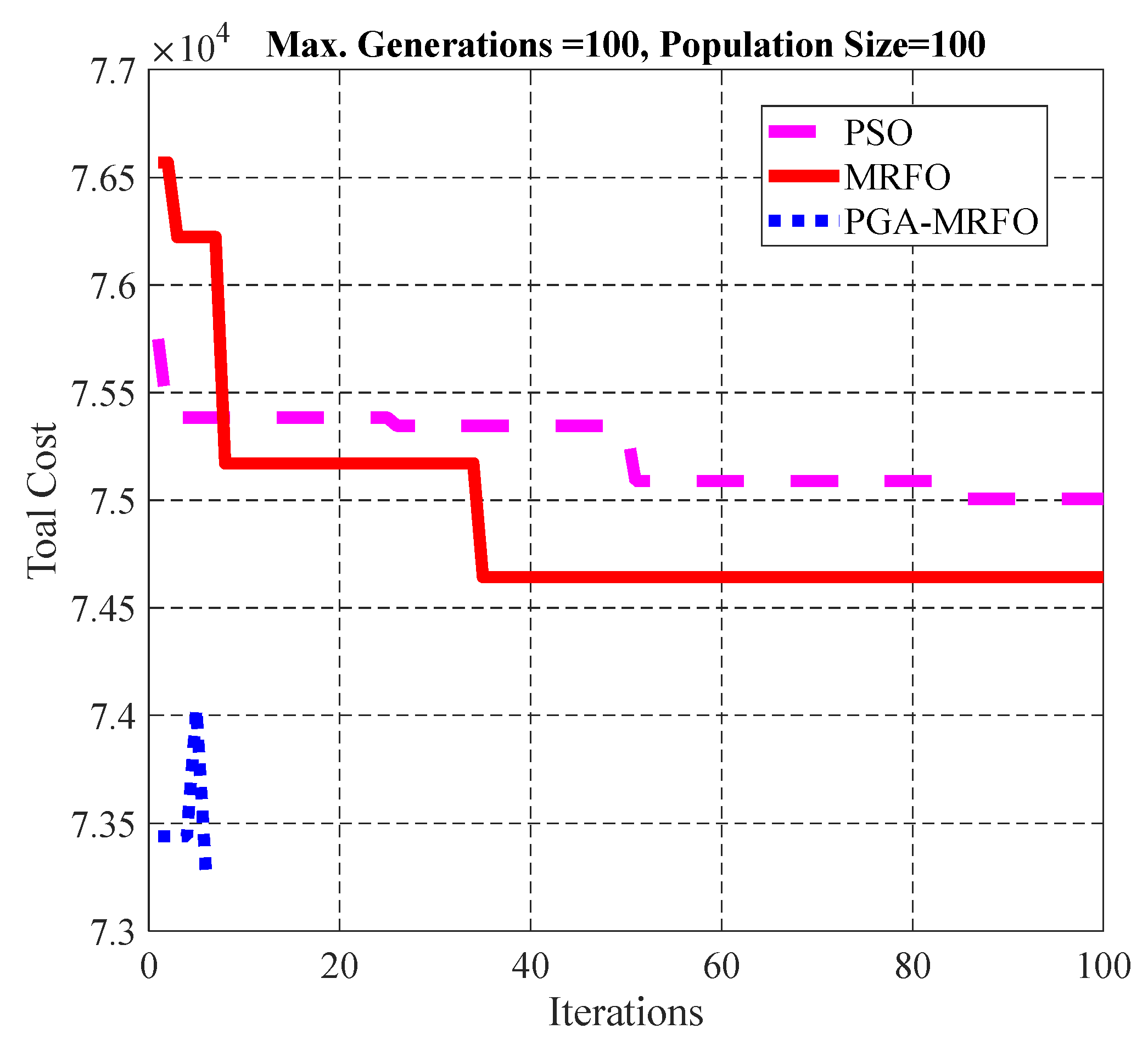
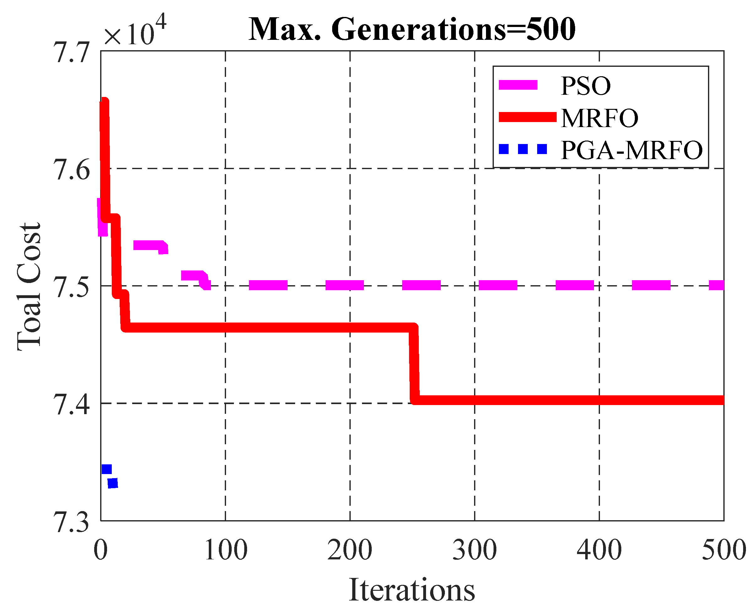
5.4.1. Results of UC Problem—Case 1
5.4.2. Results of UC Problem—Case 2
6. Analysis of the Proposed Algorithm
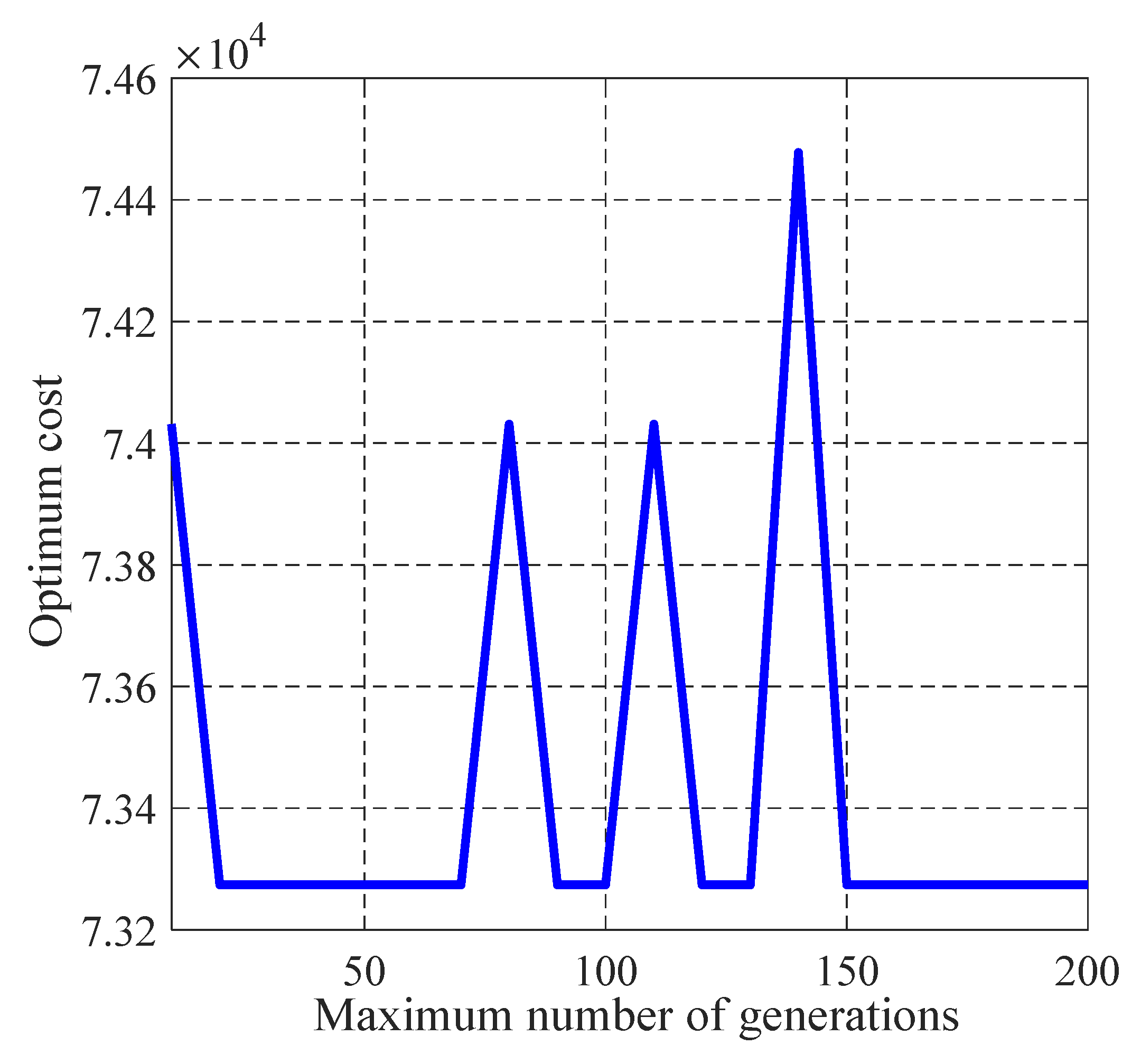
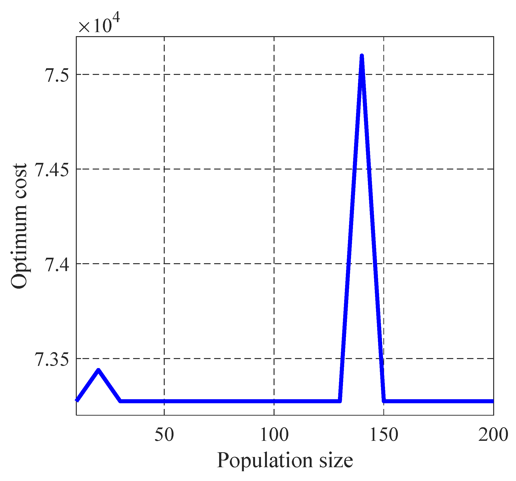
6.1. Uncertainty Analysis of the Proposed Algorithm
6.2. Robustness Analysis of the Proposed Algorithm
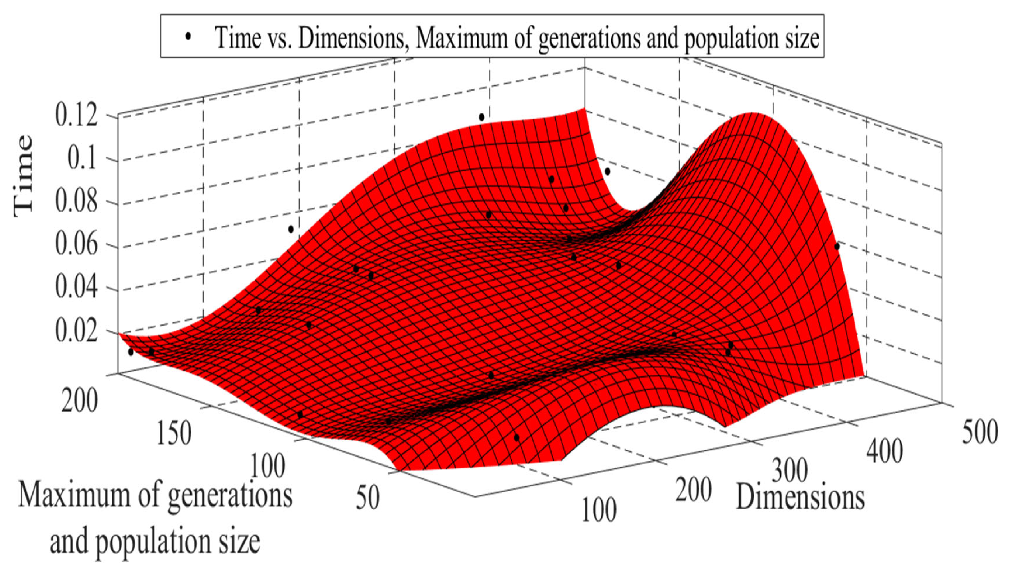
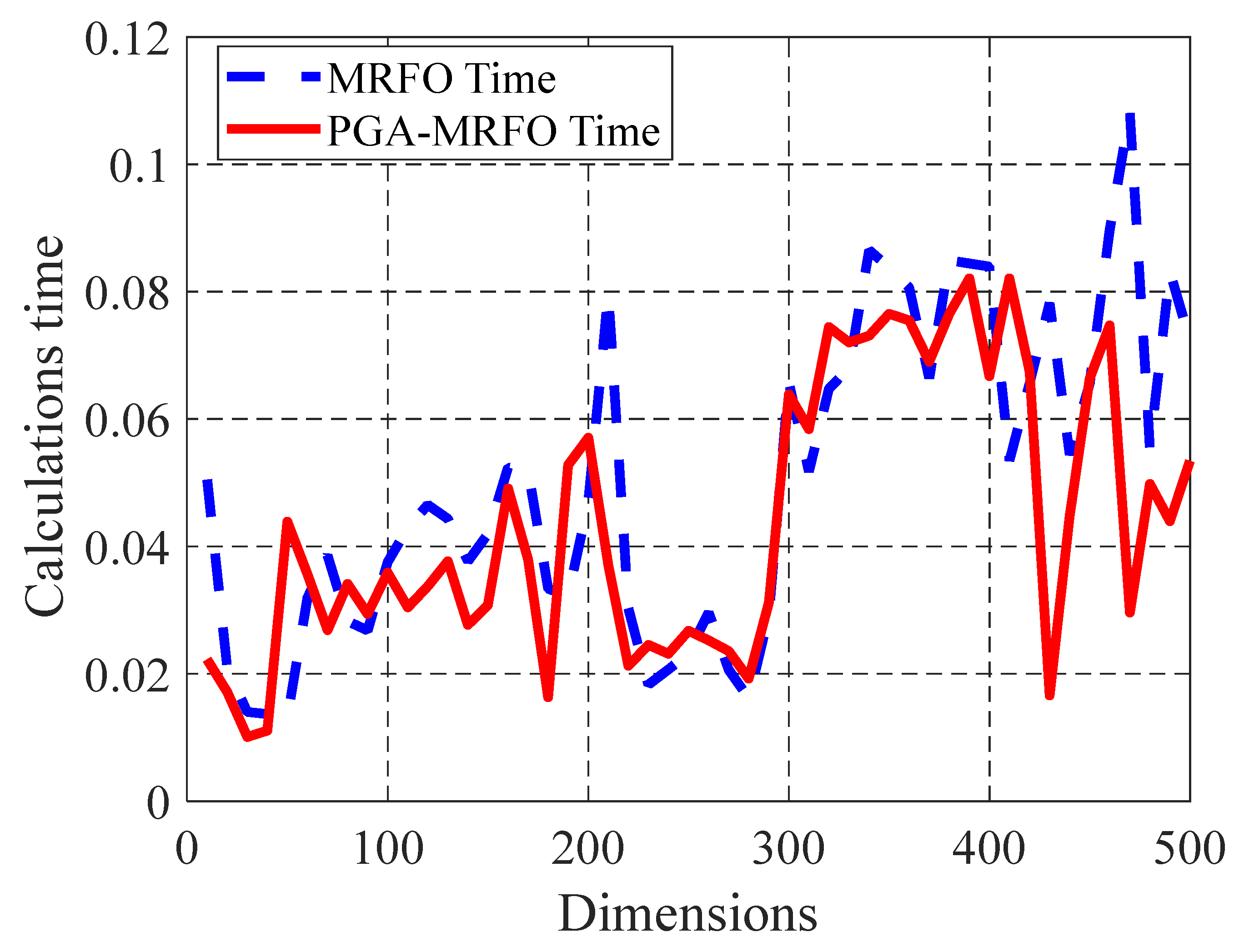
6.3. Time Complexity and Computational Time Analysis of PGA-MRFO
- The time complexity may be considered the amount of time an algorithm takes to be executed as a function of the input size. Here, the input size indicates the number of operations performed by the algorithm. The PGA-MRFO algorithm’s time complexity may be considered the result of the classical MRFO’s time complexity and the genetic algorithm’s time complexity. The genetic algorithm’s time complexity is considered as Where; D is the problem dimension, G is the maximum number of generations, and P is the population size. While in the proposed algorithm, the dimension in the genetic loop is constant (3), its time complexity reduces to be or after approximation . So, the time complexity of the PGA-MRFO algorithm is less than that of the hybridization algorithm between GA and classical MRFO.
- The actual computation time of the PGA-MRFO algorithm is calculated through different cases of a problem. Then, curve fitting is used to identify this time as a function of specific parameters. In this strategy, the parameters will be the dimensions of the problem and the maximum value between generations and population size. Since the time complexity depends on the problem dimensions and other parameters, it is essential to raise the dimensional easily to facilitate the investigation, which will not always be available in the UC problem. So, the time complexity analysis of the proposed algorithm will be discussed for the following test function:
- Another strategy to illustrate the improvement resulting from the proposed PGA-MRFO algorithm is to apply it and the MRFO algorithm to the objective function of Equation (49). The problem dimension varies from 10 to 500, yielding 50 cases, while the maximum generations and population size will be fixed at (100, 50). Figure 21 shows the comparison between PGA-MRFO and MRFO calculation time.
7. Conclusions
Author Contributions
Funding
Institutional Review Board Statement
Data Availability Statement
Conflicts of Interest
Abbreviations
| Variable | Description |
| N | Number of variables |
| The position of ith individual at time t in dth dimension | |
| Random vector within the range of [0,1] | |
| Weight coefficient | |
| The plankton with high concentration | |
| β | weight coefficient |
| T | Maximum number of iterations |
| S | Somersault factor |
| t | The current iteration |
| s | The pseudo parameter |
| α | |
| Pseudo parameter step | |
| The problem variable i | |
| The lower limit of the variable i | |
| The upper limit of the variable i | |
| The variable (i) domain | |
| Pseudo parameter domain | |
| The fitness function | |
| The pseudo function | |
| The gradient of the fitness function | |
| The pseudo-inverse (Moore-Penrose) of the approximated gradient | |
| The presumed improving ratio of objective function within range (0, 1) | |
| Vector of system variables | |
| The best solution | |
| The best fitness value | |
| The output power of generation unit i at period k | |
| The commitment state of unit i at period k | |
| The generation fuel cost of unit i at period k | |
| The startup cost of unit i at period k | |
| Number of generating units | |
| The total number of scheduling periods | |
| The no-load cost of generator i | |
| The incremental fuel cost of generator i | |
| The heat rate of the generator i | |
| The number of the ON-hours for unit i | |
| The minimum up-time for unit i | |
| The spinning reserve requirement | |
| The total load |
References
- Michael, B.-B. Nonlinear Optimization with Engineering Applications. In Springer Optimization and Its Applications; Springer: Berlin/Heidelberg, Germany, 2008. [Google Scholar]
- Rao, S.S. Engineering Optimization: Theory and Practice, 3rd ed.; Wiley: Hoboken, NY, USA, 2009. [Google Scholar]
- Michalewicz, Z. Evolutionary Computation Techniques for Nonlinear Programming Problems. Int. Trans. Oper. Res. 2008, 1, 223–240. [Google Scholar] [CrossRef] [Green Version]
- Onwubolu, G.C.; Babu, B.V. New Optimization Techniques in Engineering; Springer Science & Business Media: Berlin/Heidelberg, Germany, 2004; Volume 141. [Google Scholar]
- John, H.H. Genetic Algorithms. Sci. Am. 1992, 267, 66–73. [Google Scholar]
- Sastry, K.; Goldberg, D.; Kendall, G. Genetic Algorithms. In Search Methodologies; Burke, E.K., Kendall, G., Eds.; Springer: Boston, MA, USA, 2005. [Google Scholar]
- El-Desoky, I.M.; El-Shorbagy, M.A.; Nasr, S.M.; Hendawy, Z.M.; Mousa, A.A. A hybrid genetic algorithm for job shop scheduling problems. Int. J. Adv. Eng. Technol. Comput. Sci. 2016, 1, 6–17. [Google Scholar]
- El-Shorbagy, A.M.; Ayoub, A.Y.; El-Desoky, I.M.; Mousa, A.A. A Novel Genetic Algorithm Based K-Means Algorithm for Cluster Analysis. In International Conference on Advanced Machine Learning Technologies and Applications; Springer: Cham, Switherland, 2018; pp. 92–101. [Google Scholar]
- Storn, R.; Price, K. Differential evolution-a simple and efficient heuristic for global optimization over continuous spaces. J. Glob. Optim. 1997, 11, 341–359. [Google Scholar] [CrossRef]
- Simon, D. Evolutionary Optimization Algorithms; John Wiley & Sons, Ltd.: Hoboken, NJ, USA, 2013. [Google Scholar]
- Beni, G.; Wang, J. Swarm Intelligence in Cellular Robotic Systems. In Proceedings of the NATO Advanced Workshop on Robots and Biological Systems, Tuscany, Italy, 26–30 June 1989; Springer: Berlin/Heidelberg, Germany, 1989; pp. 703–712. [Google Scholar]
- El-Shorbagy, M.; Hassanien, A.E. Particle swarm optimization from theory to applications. Int. J. Rough Sets Data Anal. 2018, 5, 1–24. [Google Scholar] [CrossRef]
- El-Shorbagy, M.A.; El-Shorbagy, M. Weighted Method Based Trust Region-Particle Swarm Optimization for Multi-Objective Optimization. Am. J. Appl. Math. 2015, 3, 81. [Google Scholar] [CrossRef]
- Allah, A.M.A.; El-Shorbagy, M.A. Enhanced Particle Swarm Optimization Based Local Search for Reactive Power Compensation Problem; Scientific Research Publishing: Wuhan, China, 2012. [Google Scholar]
- Dorigo, M.; Stutzle, T. Ant Colony Optimization; MIT Press: Cambridge, MA, USA, 2004. [Google Scholar]
- Saremi, S.; Mirjalili, S.; Lewis, A. Grasshopper Optimisation Algorithm: Theory and application. Adv. Eng. Softw. 2017, 105, 30–47. [Google Scholar] [CrossRef] [Green Version]
- Zhao, W.; Zhang, Z.; Wang, L. Manta ray foraging optimization: An effective bio-inspired optimizer for engineering applications. Eng. Appl. Artif. Intell. 2020, 87, 103300. [Google Scholar] [CrossRef]
- Zhang, Y.; Jin, Z. Group teaching optimization algorithm: A novel metaheuristic method for solving global optimization problems. Expert Syst. Appl. 2020, 148, 113246. [Google Scholar] [CrossRef]
- Atashpaz-Gargari, E.; Lucas, C. Imperialist competitive algorithm: An algorithm for optimization inspired by imperialistic competition. In Proceedings of the 2007 IEEE Congress on Evolutionary Computation, Singapore, 25–28 September 2007; pp. 4661–4667. [Google Scholar]
- Rao, R.; Savsani, V.; Vakharia, D. Teaching–Learning-Based Optimization: An optimization method for continuous non-linear large scale problems. Inf. Sci. 2012, 183, 1–15. [Google Scholar] [CrossRef]
- Kashan, A.H. An efficient algorithm for constrained global optimization and application to mechanical engineering design: League championship algorithm (LCA). Comput. Des. 2011, 43, 1769–1792. [Google Scholar]
- Askari, Q.; Younas, I.; Saeed, M. Political Optimizer: A novel socio-inspired meta-heuristic for global optimization. Knowl.-Based Syst. 2020, 195, 105709. [Google Scholar] [CrossRef]
- Rashedi, E.; Nezamabadi-Pour, H.; Saryazdi, S. GSA: A Gravitational Search Algorithm. Inf. Sci. 2009, 179, 2232–2248. [Google Scholar] [CrossRef]
- Tayarani-N, M.H.; Akbarzadeh-T, M.R. Magnetic Optimization Algorithms a New Synthesis. In Proceedings of the2008 IEEE Congress on Evolutionary Computation (IEEE World Congress on Computational Intelligence), Hong Kong, China, 1–6 June 2008; pp. 2659–2664. [Google Scholar]
- Van Laarhoven, P.J.M.; Aarts, E.H.L. Simulated Annealing. In Simulated Annealing: Theory and Applications; Springer: Dordrecht, The Netherlands, 1978; pp. 7–15. [Google Scholar]
- Izci, D.; Ekinci, S.; Eker, E.; Kayri, M. Improved manta ray foraging optimization using opposition-based learning for optimization problems. In Proceedings of the 2020 International Congress on Human-Computer Interaction Optimization and Robotic Applications (HORA), Ankara, Turkey, 26–27 June 2020; pp. 1–6. [Google Scholar]
- Mohamed; Hassan, H.; Essam; Houssein, H.; Mohamed; Mahdy, A.; Kamel, S. An improved Manta ray foraging optimizer for cost-effective emission dispatch problems. Eng. Appl. Artif. Intell. 2021, 100, 1–20. [Google Scholar]
- Muralikrishnan, N.; Jebaraj, L.; Rajan, C.C.A. A Comprehensive Review on Evolutionary Optimization Techniques Applied for Unit Commitment Problem. IEEE Access 2020, 8, 132980–133014. [Google Scholar] [CrossRef]
- Shadaksharappa, N.M. Optimum Generation Scheduling for Thermal Power Plants using Artificial Neural Network. Int. J. Electr. Comput. Eng. 2011, 1, 134–139. [Google Scholar] [CrossRef]
- Dudek, G. Adaptive simulated annealing schedule to the unit commitment problem. Electr. Power Syst. Res. 2010, 80, 465–472. [Google Scholar] [CrossRef]
- Sakthi, S.S.; Santhi, R.; Krishnan, N.M.; Ganesan, S.; Subramanian, S. Wind Integrated Thermal Unit Commitment Solution Using Grey Wolf Optimizer. Int. J. Electr. Comput. Eng. 2017, 7, 2309. [Google Scholar] [CrossRef]
- Ponciroli, R.; Stauff, N.E.; Ramsey, J.; Ganda, F.; Vilim, R.B. An Improved Genetic Algorithm Approach to the Unit Commitment/Economic Dispatch Problem. IEEE Trans. Power Syst. 2020, 35, 4005–4013. [Google Scholar] [CrossRef]
- Zhai, Y.; Liao, X.; Mu, N.; Le, J. A two-layer algorithm based on PSO for solving unit commitment problem. Soft Comput. 2020, 24, 9161–9178. [Google Scholar] [CrossRef]
- Kamboj, V.K. A novel hybrid PSO–GWO approach for unit commitment problem. Neural Comput. Appl. 2016, 27, 1643–1655. [Google Scholar] [CrossRef]
- Khunkitti, S.; Watson, N.R.; Chatthaworn, R.; Premrudeepreechacharn, S.; Siritaratiwat, A. An Improved DA-PSO Optimization Approach for Unit Commitment Problem. Energies 2019, 12, 2335. [Google Scholar] [CrossRef] [Green Version]


| Test Function | Function No. | D | Domain | NO. of Iterations Using MRFO | NO. of Iterations Using PGA-MRFO | Percentage Improvement |
|---|---|---|---|---|---|---|
| Rosenbrok | F5 | 30 | 1000 | 438 | 56.2% | |
| Quartic | F7 | 30 | [−1.28,1.28] | 1000 | 419 | 58.1% |
| Schwefel | F8 | 30 | 1000 | 520 | 48% | |
| Penalized2 | F13 | 30 | [−50,50] | 1000 | 181 | 81.9% |
| Foxholes | F14 | 2 | [−65.536,65.536] | 62 | 42 | 32.2% |
| Kowalik | F15 | 4 | [−5,5] | 1000 | 169 | 83.1% |
| Hartman 6 | F20 | 6 | [0,1] | 500 | 35 | 93% |
| Shekel 5 | F21 | 4 | [0,10] | 1000 | 109 | 89.1% |
| Shekel 7 | F22 | 4 | [0,10] | 325 | 165 | 49.2% |
| Shekel 10 | F23 | 4 | [0,10] | 1000 | 87 | 91.3% |
| Test Function | Function | D | Domain | NO. of Iterations Using MRFO | NO. of Iterations Using GA | NO. of Iterations Using PGA-MRFO | Percentage Improvement between PGA-MRFO and | |
|---|---|---|---|---|---|---|---|---|
| MRFO | GA | |||||||
| Sphere | F1 | 100 | 50 | 50 | 7 | 86% | 86% | |
| Schwefel 2.22 | F2 | 100 | [−10, 10] | 50 | 50 | 3 | 94% | 94% |
| Schwefel 1.2 | F3 | 100 | 50 | 50 | 5 | 90% | 90% | |
| Schwefel 2.21 | F4 | 100 | ] | 50 | 50 | 6 | 88% | 88% |
| Rosenbrock | F5 | 100 | 50 | 50 | 4 | 92% | 92% | |
| Step | F6 | 100 | [−100, 100] | 50 | 50 | 5 | 90% | 90% |
| Quartic | F7 | 100 | 50 | 50 | 22 | 56% | 56% | |
| Schwefel | F8 | 100 | 50 | 30 | 30 | 44% | 0% | |
| Rastrigin | F9 | 100 | 50 | 50 | 3 | 94% | 94% | |
| Ackley | F10 | 100 | 50 | 50 | 7 | 86% | 86% | |
| Griewank | F11 | 100 | 50 | 50 | 7 | 86% | 86% | |
| Penalized | F12 | 100 | 50 | 50 | 17 | 66% | 66% | |
| Penalized2 | F13 | 100 | 50 | 50 | 10 | 80% | 80% | |
| Unit 1 | Unit 2 | Unit 3 | Unit 4 | |
|---|---|---|---|---|
| Pgmin [MW] | 25 | 60 | 75 | 20 |
| Pgmax [MW] | 80 | 250 | 300 | 60 |
| Inc. Heat rate [BTU/kWh] | 10,440 | 9000 | 8730 | 11,900 |
| Fuel cost [£/MBTU] | 2 | 2 | 2 | 2 |
| No load cost [£/h] | 213 | 585.62 | 684.74 | 252 |
| Min up time [h] | 4 | 5 | 5 | 1 |
| Min down time [h] | 2 | 3 | 4 | 1 |
| Startup cost [£] | 150 | 170 | 500 | 0 |
| Unit 1 | Unit 2 | Unit 3 | Unit 4 | Unit 5 | Unit 6 | Unit 7 | Unit 8 | Unit 9 | Unit 10 | |
|---|---|---|---|---|---|---|---|---|---|---|
| Pgmin [MW] | 30 | 130 | 165 | 130 | 225 | 50 | 250 | 110 | 275 | 75 |
| Pgmax [MW] | 100 | 400 | 600 | 420 | 700 | 200 | 750 | 375 | 850 | 250 |
| Inc. Heat rate [BTU/kWh] | 9000 | 10,000 | 1100 | 1120 | 1800 | 340 | 520 | 60 | 60 | 60 |
| Fuel cost [£/MBTU] | 2 | 2 | 2 | 2 | 2 | 2 | 2 | 2 | 2 | 2 |
| No load cost [£/h] | 1000 | 970 | 700 | 680 | 450 | 370 | 480 | 660 | 665 | 670 |
| Min up time [h] | 5 | 3 | 2 | 1 | 4 | 2 | 3 | 1 | 4 | 2 |
| Min down time [h] | 4 | 2 | 4 | 3 | 5 | 2 | 4 | 3 | 3 | 1 |
| Startup cost [£] | 2050 | 1460 | 2100 | 1480 | 2100 | 1360 | 2300 | 1370 | 2200 | 1180 |
| Max. Generations = 100 | ||||
| Algorithm | DP | PSO | MRFO | PGA-MRFO |
| Total cost | 74,110 | 75,006 | 74,643 | 73,274 |
| Consumed iterations | - | 100 | 100 | 6 |
| Max. Generations = 300 | ||||
| Algorithm | DP | PSO | MRFO | PGA-MRFO |
| Total cost | 74,110 | 75,006 | 73,559 | 73,274 |
| Consumed iterations | - | 300 | 300 | 7 |
| Max. Generations = 500 | ||||
| Algorithm | DP | PSO | MRFO | PGA-MRFO |
| Total cost | 74,110 | 75,006 | 74,027 | 73,274 |
| Consumed iterations | - | 500 | 500 | 10 |
| Max. Generations = 100 | ||||
| Algorithm | DP | PSO | MRFO | PGA-MRFO |
| Total cost | 38,271 | 91,152 | 42,514 | 37,765 |
| Max. Generations = 300 | ||||
| Algorithm | DP | PSO | MRFO | PGA-MRFO |
| Total cost | 38,271 | 91,152 | 49,993 | 36,304 |
| Max. Generations = 500 | ||||
| Algorithm | DP | PSO | MRFO | PGA-MRFO |
| Total cost | 38,271 | 91,152 | 49,993 | 36,303 |
| Algorithm | DP Optimum Cost | PSO Optimum Cost | MRFO Optimum Cost | PGA-MRFO Optimum Cost |
|---|---|---|---|---|
| Uncertainty Load Percentage | ||||
| Original case (0%) | 74,110 | 74,721 | 74,207 | 73,274 |
| Original case ± 1% | 74,070 | 73,961 | 74,589 | 74,059 |
| Original case ± 2% | 74,031 | 73,885 | 74,531 | 73,982 |
| Original case ± 3% | 75,020 | 74,246 | 74,524 | 74,344 |
| Original case ± 4% | 72,972 | 75,641 | 75,075 | 74,141 |
| Original case ± 5% | 75,176 | 74,054 | 73,190 | 72,256 |
| Original case ± 6% | 72,538 | 76,414 | 75,914 | 74,981 |
| Original case ± 7% | 75,766 | 74,583 | 73,968 | 73,034 |
| Original case ± 8% | 73,416 | 74,404 | 74,157 | 73,224 |
| Original case ± 9% | 76,778 | 75,441 | 75,742 | 74,865 |
| Original case ± 10% | 74,734 | 77,390 | 76,969 | 75,765 |
| Original case ± 11% | 73,902 | 75,001.9 | 74,865.9 | 74,065.1 |
| Original case ± 12% | 76,283 | 74,629 | 74,280 | 72,712 |
| Original case ± 13% | 76,290 | 77,857 | 77,406 | 76,253 |
| Original case ± 14% | 75,773 | 77,185 | 76,468 | 75,535 |
| Original case ± 15% | 74,099 | 76,839 | 77,237 | 75,842 |
| Original case ± 16% | 74,099 | 71,984 | 71,366 | 70,446 |
| Original case ± 17% | 77,743 | 80,247 | 79,536 | 78,603 |
| Original case ± 18% | 76,210 | 77,568 | 76,980 | 75,650 |
| Original case ± 19% | 71,211 | 69,903 | 69,195 | 67,618 |
| Original case ± 20% | 76,803 | 76,699 | 75,563 | 74,629 |
| Mean | 74,845.7 | 75,396.6 | 75,077.795 | 74,100.205 |
| Standard deviation | 2288.401536 | 2271.454 | 2247.9908 | 1641.46196 |
| Algorithm | DP Optimum Cost | PSO Optimum Cost | MRFO Optimum Cost | PGA-MRFO Optimum Cost |
|---|---|---|---|---|
| Uncertainty Fuel Cost Percentage | ||||
| Original case (0%) | 74,110 | 74,721 | 74,207 | 73,274 |
| Original case ± 1% | 73,866 | 74,499 | 73,989 | 73,051 |
| Original case ± 2% | 75,104 | 75,696 | 75,188 | 74,288 |
| Original case ± 3% | 73,672 | 74,423 | 73,944 | 72,974 |
| Original case ± 4% | 74,527 | 75,073 | 74,872 | 73,647 |
| Original case ± 5% | 74,080 | 74,601 | 74,343 | 73,074 |
| Original case ± 6% | 74,372 | 75,056 | 74,622 | 73,672 |
| Original case ± 7% | 72,515 | 73,216 | 72,688 | 71,659 |
| Original case ± 8% | 74,140 | 75,054 | 74,681 | 73,737 |
| Original case ± 9% | 75,986 | 76,919 | 76,621 | 76,323 |
| Original case ± 10% | 74,621 | 75,853 | 74,956 | 75,115 |
| Original case ± 11% | 74,907 | 75,572 | 75,069 | 74,113 |
| Original case ± 12% | 72,092 | 72,655 | 72,304 | 70,981 |
| Original case ± 13% | 72,012 | 73,304 | 73,099 | 72,724 |
| Original case ± 14% | 73,760 | 74,866 | 74,777 | 73,881 |
| Original case ± 15% | 81,207 | 81,960 | 81,648 | 80,780 |
| Original case ± 16% | 82,712 | 84,993 | 84,088 | 82,424 |
| Original case ± 17% | 74,027 | 76,146 | 74,147 | 72,636 |
| Original case ± 18% | 75,351 | 75,882 | 76,222 | 74,607 |
| Original case ± 19% | 77,183 | 80,019 | 78,332 | 77,228 |
| Original case ± 20% | 65,573 | 66,482 | 66,288 | 65,425 |
| Mean | 74,596.5 | 75,670.78 | 75,150.06 | 74,166.67 |
| Standard deviation | 3471.103 | 3686.144 | 3536.355 | 3408.60549 |
| Parameter | Mean | Standard Deviation | Error |
|---|---|---|---|
| Maximum number of Generations | 73,447.75 | 367.4222 | 0.002371 |
| Population size | 73,373.55 | 408.031 | 0.001358 |
| 73,377.1 | 329.5517 | 0.001407 |
| Coefficient | |||||||
| Value | 2.292 | 0.3527 | 1.301 | −0.3958 | −0.5647 | −0.7977 | 0.1382 |
| Coefficient | |||||||
| Value | −1.22 | 0.466 | −0.5679 | 0.2399 | −0.3286 | −0.06093 | 0.8375 |
| Coefficient | |||||||
| Value | 0.670 | 0.07944 | 0.03898 | −0.2443 | 0.4315 | 0.16 | 0.3069 |
| Algorithm | MRFO | PGA-MRFO |
|---|---|---|
| Mean value | 0.050418 | 0.043794 |
| Standard deviation | 0.02474438 | 0.021480797 |
Publisher’s Note: MDPI stays neutral with regard to jurisdictional claims in published maps and institutional affiliations. |
© 2022 by the authors. Licensee MDPI, Basel, Switzerland. This article is an open access article distributed under the terms and conditions of the Creative Commons Attribution (CC BY) license (https://creativecommons.org/licenses/by/4.0/).
Share and Cite
El-Shorbagy, M.A.; Omar, H.A.; Fetouh, T. Hybridization of Manta-Ray Foraging Optimization Algorithm with Pseudo Parameter-Based Genetic Algorithm for Dealing Optimization Problems and Unit Commitment Problem. Mathematics 2022, 10, 2179. https://doi.org/10.3390/math10132179
El-Shorbagy MA, Omar HA, Fetouh T. Hybridization of Manta-Ray Foraging Optimization Algorithm with Pseudo Parameter-Based Genetic Algorithm for Dealing Optimization Problems and Unit Commitment Problem. Mathematics. 2022; 10(13):2179. https://doi.org/10.3390/math10132179
Chicago/Turabian StyleEl-Shorbagy, Mohammed A., Hala A. Omar, and Tamer Fetouh. 2022. "Hybridization of Manta-Ray Foraging Optimization Algorithm with Pseudo Parameter-Based Genetic Algorithm for Dealing Optimization Problems and Unit Commitment Problem" Mathematics 10, no. 13: 2179. https://doi.org/10.3390/math10132179
APA StyleEl-Shorbagy, M. A., Omar, H. A., & Fetouh, T. (2022). Hybridization of Manta-Ray Foraging Optimization Algorithm with Pseudo Parameter-Based Genetic Algorithm for Dealing Optimization Problems and Unit Commitment Problem. Mathematics, 10(13), 2179. https://doi.org/10.3390/math10132179