Abstract
With the emergence of various online trading technologies, fraudulent cases begin to occur frequently. The problem of fraud in public trading companies is a hot topic in financial field. This paper proposes a fraud detection model for public trading companies using datasets collected from SEC’s Accounting and Auditing Enforcement Releases (AAERs). At the same time, this computational finance model is solved with a nonlinear activated Beetle Antennae Search (NABAS) algorithm, which is a variant of the meta-heuristic optimization algorithm named Beetle Antennae Search (BAS) algorithm. Firstly, the fraud detection model is transformed into an optimization problem of minimizing loss function and using the NABAS algorithm to find the optimal solution. NABAS has only one search particle and explores the space under a given gradient estimation until it is less than an “Activated Threshold” and the algorithm is efficient in computation. Then, the random under-sampling with AdaBoost (RUSBoost) algorithm is employed to comprehensively evaluate the performance of NABAS. In addition, to reflect the superiority of NABAS in the fraud detection problem, it is compared with some popular methods in recent years, such as the logistic regression model and Support Vector Machine with Financial Kernel (SVM-FK) algorithm. Finally, the experimental results show that the NABAS algorithm has higher accuracy and efficiency than other methods in the fraud detection of public datasets.
Keywords:
fraud detection; nonlinear activated beetle antennae search; unbalanced dataset; computational finance MSC:
91G40; 90C26
1. Introduction
In recent years, people rely more on the Internet for the development of modern technologies, which not only brings great convenience to people’s lives but also brings great risks. In the financial field, it has led to a lot of fraudulent financial activities [1], such as mobile payment fraud [2], telecom fraud [3] and credit card fraud [4]. The detection of fraudulent financial activities is thus necessary. In [5], Ngai et al. proposed that financial fraud detection (FFD) distinguishes false financial information from real data and reveals financial fraud activities, which plays an important role in preventing the serious consequences of financial fraud. In particular, the fraud detection [6] of public trading companies is a hot issue in FDD. In [7], Reurink pointed out that company managers may provide false financial statements due to insider trading, performance pressure, or financial difficulties. The fraudulent behavior will not only directly harm the interests of investors, but also affect fair competition with other non-fraudulent companies. However, due to the wide gap between fraudulent companies and non-fraudulent companies, and the complexity and diversity of fraudulent activities, it is difficult to judge fraudulent companies in a short time.
In order to achieve the correct classification of the specified type, huge datasets are used for training. In general, the datasets used for classification are divided into the labeled and unlabeled dataset. Machine learning (ML) is a method that learns from training datasets to complete prediction tasks. It is an effective solution for fraud detection and prevention, and is now increasingly used in the fraud detection of the financial industry. Based on unlabeled datasets, an unsupervised machine learning method named autoencoder was used to accurately detect fraudulent events [8]. Meanwhile, other ML methods include decision tree, random forest, and XGBoost algorithm, which based on labeled datasets were also used in fraud detection [9]. According to the efficient classification and prediction of machine learning, in this paper, a model based on ML methods is proposed, and the confusion matrix in machine learning and its related evaluation indicators are used to evaluate the performance of the model.
It is worth noting because of the difficulty for technicians to gather enough useful information from the real environment, learning and analysis based on unbalanced datasets are ubiquitous [10]. Meanwhile, in [11], various ML methods were used for the classification and prediction of unbalanced datasets. The results showed that no matter which method is used, the impact of unbalanced datasets on prediction accuracy cannot be eliminated. Therefore, it is necessary to formulate specific strategies for special unbalanced datasets. This paper employs an over-sampling technique to deal with unbalanced datasets and sets an appropriate threshold to adjust for the bias between fraudulent and non-fraudulent companies. In this way, the number of samples of fraudulent and non-fraudulent companies can be balanced as much as possible, thereby reducing the impact of unbalanced datasets on the classification and prediction results of ML methods.
Different from the existing ML methods mentioned above, this paper presents an improved Beetle Antennae Search (BAS) algorithm to solve the optimization problem. The Beetle Antennae Search algorithm is a meta-heuristic algorithm, which was proposed by Jiang et al. [12]. It simulates the behavior of the beetles using antennae to search for food in nature and only has one particle for global search. Thus, this algorithm has the advantage of quick convergence properties and simple implementation compared to other swarm optimization algorithms [13]. In recent years, in the financial field, the BAS algorithm has been applied to the portfolio insurance problem [14,15,16,17,18,19]. However, the research on public trade audit companies is limited and few studies use the BAS algorithm for fraud detection [20]. Additionally, the original BAS algorithm has shortcomings like premature convergence and easy falling into local minima. In this paper, a variant of BAS named nonlinear activated Beetle Antennae Search (NABAS) is presented to solve the fraud detection problem of public trading companies. The NABAS algorithm introduces a nonlinear “Activated Threshold” based on the step size update rule of BAS. When the gradient value is less than the threshold, the algorithm is allowed to update the search step size. This improvement helps NABAS avoid a fast convergence rate and be immune to local minima.
Over the years, many studies have proposed solutions to the problem of fraud detection in public trading companies. Dechow et al. created a dataset from 1982 to 2005 about fraudulent companies, which was collected from Accounting and Auditing Enforcement Releases (AAERs) issued by the Securities and Exchange Commission (SEC) [21]. The dataset summarized the characteristics that could best distinguish fraudulent companies from non-fraudulent companies, and these characteristics were used as variables in the logistic regression model based on financial ratios. After that, a financial kernel was created by Cecchini in [22], which could implicitly map relevant financial attributes to ratios. Then, the constructed kernel function was used as part of a support vector machine (SVM-FK) to detect fraud. Moreover, a new ensemble learning method named Random Under-Sampling with AdaBoost (RUSBoost) was adopted in [23], and it is a boosting-based sampling algorithm for dealing with unbalanced data in class tag datasets. According to the fraud detection in public trading companies in this paper, the three methods including the logistic regression model, SVM-FK, and RUSBoost are used as the benchmark to compare with NABAS.
The rest of this paper is organized as follows: Section 2 introduces the efficient way to handle an unbalanced dataset and formulate a model for this fraud detection problem. Section 3 introduces the original BAS algorithm and further presents the NABAS algorithm. Section 4 applies the NABAS algorithm to the fraud detection model and compared it with RUSBoost, logistic regression model, and SVM-FK. Section 5 summarizes the work of this paper.
2. Unbalanced Dataset and Model Establishment
In this section, firstly, the nature and processing method of the highly unbalanced dataset are given. Moreover, combined with the confusion matrix, the performance evaluation indicators of the model are analyzed. Finally, a loss function is designed to get the optimal solution to this fraud detection problem.
2.1. Highly Unbalanced Dataset
In this paper, we use a typical unbalanced dataset, which is collected from SEC’s AAERs [23]. It contains a total of 206,026 public trading USA companies, with 204,855 non-fraudulent companies but only 1171 fraudulent companies from 1979 to 2014. The dataset is shown in Table 1. Particularly, the dataset contains 28 raw financial variables and 14 financial ratios.

Table 1.
Distribution of fraudulent companies by year from 1979–2014 [23].
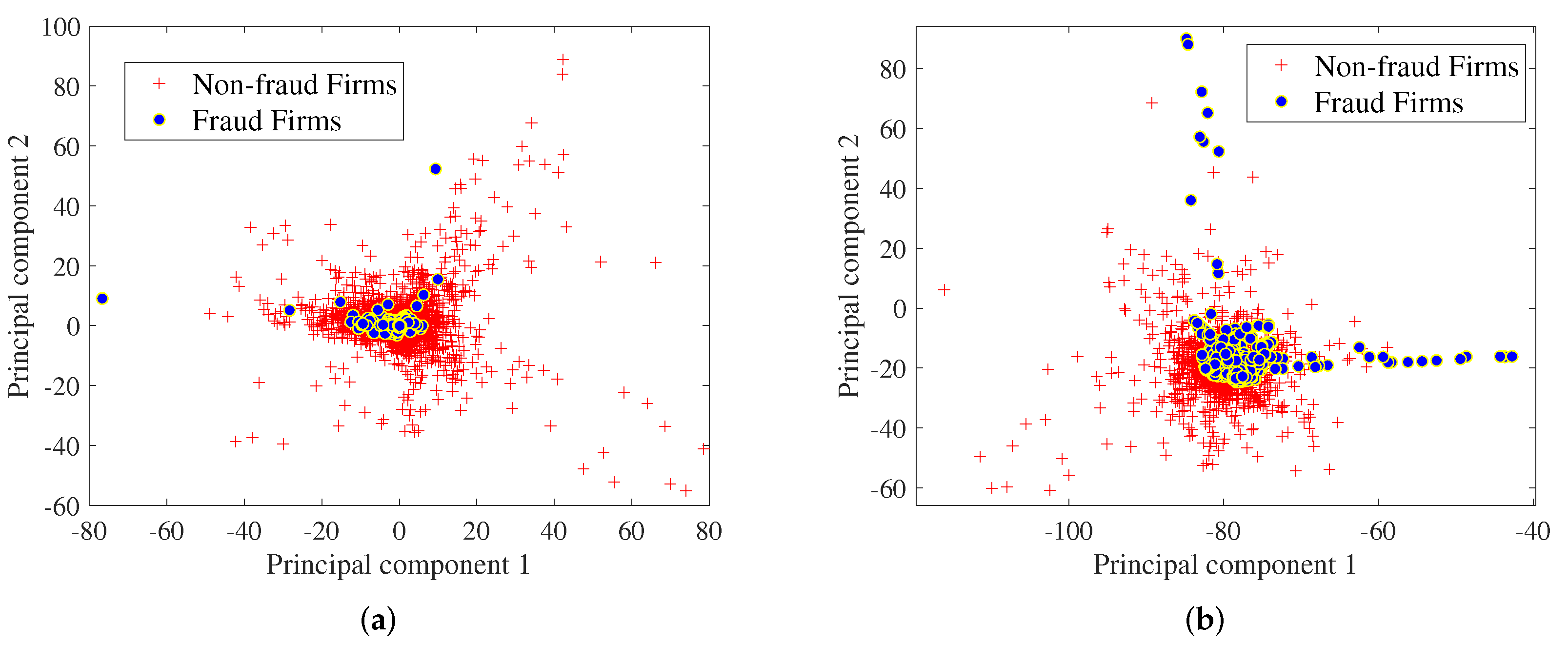
In [23], the financial ratios applied to the fraud prediction model are more powerful than the raw financial variables. However, the ratios were identified by experts; it thus lacks lots of useful information. In order to ensure the integrity of the dataset, these 28 raw financial variables are used as the dataset for the fraud detection of public trading companies. This means we have to handle a 28-dimensional dataset which is complex to show each component of it. To display the data information more clearly, a technique called principal component analysis (PCA) is used to visualize this dataset [24]. The characteristic of PCA is to extract the main feature components of data from complex high-dimensional information, which contains most of the useful information in the dataset. After processing by PCA, two of the principal components were extracted from the 28-dimensional dataset, and the results are displayed in Figure 1a. From the picture, one can find that the information among the samples overlaps, and the number of two categories has a huge gap; it is difficult to deal with them directly. Thus, formulating a targeted sample processing strategy for the specific issue is necessary.
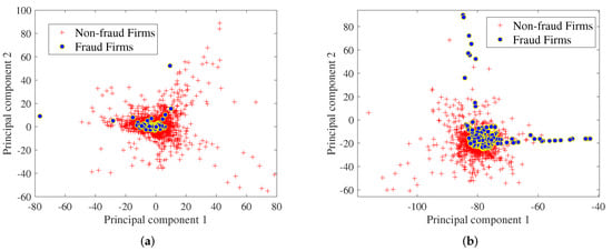
Figure 1.
Visualization of the unbalanced dataset, the red plus signs represent non-fraudulent companies and the blue points represent fraudulent companies. (a) Visualization of 28-dimensional samples in the original dataset; (b) visualization of the dataset after the samples are processed by a SMOTE technique.
Here are several sampling techniques of processing to deal with the unbalanced dataset, e.g., under-sampling techniques, over-sampling techniques, and another over-sampling technique named Synthetic Minority Over-sampling Technique (SMOTE) [25]. The simple introductions of these techniques are as follows:
2.1.1. Under-Sampling Technique
For majority classes in unbalanced datasets, the under-sampling technique randomly reduces the number of majority classes until it was consistent with the minority class. In this dataset, we should use the under-sampling technique to reduce 204,855 non-fraudulent companies to 1171, which is equivalent to fraudulent companies. This technique is easy to implement, but a large amount of useful data will be lost in the under-sampling process.
2.1.2. Over-Sampling Technique
The process of this technique is oppositive to under-sampling, which aims at increasing the number of the minority classes, by directly repeating the relevant information until the number is equal to the majority classes. This is an efficient way to balance the numbers of these two categories. However, after over-sampling dealing with the unbalanced dataset, the class obtained from the minority class is highly repetitive, and the prediction result is easy to over-fit.
2.1.3. Over-Sample Data with SMOTE Technique
At present, the over-sampling technique is used frequently in various fields. However, blindly adding new samples may be ineffective or produce noise to the dataset. In this problem, the SMOTE technique is used to oversample the minority class. Firstly, for each minority class sample, SMOTE takes the Euclidean distance as the standard and selects another sample from its nearest neighbor. In addition, it then randomly generates a point on the connection line between the two as the new composite sample. Finally, iterating continuously, until the few classes are sampled to most classes. Compared with the conventional over-sampling technique, SMOTE helps the classification models obtain higher prediction accuracy. It combines the characteristics of different samples to provide a diversity of data better. After tackling with SMOTE, the new dataset is shown in Figure 1b. It can be seen that the number of fraud companies has increased and the overlap between new samples has decreased.
2.2. Model Evaluation
In machine learning, it is crucial to choose an evaluation method that matches the problem, which helps to quickly find the key in the model selection or training process. For the binary confusion matrix, true positive (TP) is the number of fraudulent companies that are correctly classified as fraudulent companies, true negative (TN) is the number of non-fraudulent companies that are classified as non-fraudulent companies, false positive (FP) is the number of non-fraudulent companies that are misclassified as fraudulent companies, and false negative (FN) is the number of fraudulent companies that are misclassified as non-fraudulent companies [26]. This paper chooses four evaluation indicators that are closely related to the binary confusion matrix to evaluate the performance of the model. (1) Accuracy: Accuracy refers to the proportion of correctly classified samples to the total number of samples. It is the most basic index of all model evaluation indicators. However, when the sample proportion in different categories is extremely unbalanced, the category with a large proportion tends to be the most important factor affecting the accuracy. (2) Precision and Sensitivity: Precision refers to the proportion of the number of positive samples that are correctly classified to the number of positive samples determined by the classifier. Sensitivity refers to the ratio of the number of positive samples which are correctly predicted to the number of samples labeled as positive. Precision requires the detection of positive samples as accurately as possible, and sensitivity is expected to test the positive samples more comprehensively. The higher the value of both, the better the performance of the model. Precision and sensitivity are negatively correlated, so we need to find a balance to make them as high as possible at the same time. (3) NDCG: NDCG is a normalization of the Discounted Cumulative Gain (DCG) measure; it is usually used to measure and evaluate search results [27]. The DCG at the position k is defined as , where represents the correlation score of each item in the list and k is the number of top item in the list. Then, the NDCG at the position k is calculated by , where is the DCG value when all the correctly predicted positive samples are ranked at the top of the ranking list.
2.3. Optimization Problem
Since this problem is only necessary to judge whether the type of a public trading company is a fraudulent company, it is a labeled binary classification problem.
2.3.1. Binary Classification
In a binary classification problem of dimension n, the feature sample and its corresponding label . In general, a linear decision function is used to tackle the binary classification problem, which is presented as
where is the decision variables and b is a bias. Substituting (1) into the sigmoid function , we obtain
which maps the decision function (1) to .
Because of the special characteristics of the unbalanced dataset, even though the dataset is handled by SMOTE, there is still a great difference between the number of fraudulent companies and non-fraudulent companies. Therefore, a threshold is introduced to help classify the two categories. Here, we can obtain a new decision rule as
where expresses non-fraudulent companies and expresses fraudulent companies. Generally, when , the probability of judging two categories is equal. However, in this dataset, it is known that there exist characteristics like nonlinear and highly overlapping between each variable. To make the whole decision rule more inclined towards the category determination of fraudulent companies, will be set smaller than . The impact of the unbalanced dataset can thus be reduced.
2.3.2. Loss Function
In general, for classification and regression problems, the loss function is defined as
which is used to minimize to get the optimal value for each parameter of the model. In this problem, the loss function on the results of two different classes needs to be calculated at the same time. Then, we improve the function to a convex function, to help obtain the global optimal solution. The loss function is finally determined as
In addition, we consider true positive rate (TPR) and false positive rate (FPR) as
For this problem, TPR shows that the model correctly predicts the number of fraudulent companies in the dataset, while FPR is the opposite of TPR.
Then, the accuracy is used for this model; it is aimed at correctly predicting the number of positive class (fraud) and negative class (non-fraud) as much as possible at the same time, which is defined as
The higher the accuracy, the better the model performance. While the loss function needs to obtain the minimization of the solution, we should make to be reciprocal, and it is finally given as
where represents the reciprocal of . Giving different weights to formulas (2) and (3), and adding them together, one can obtain a new loss function:
The loss function (4) is transformed into an optimization problem with a constraint
where the is the ith element of vector . Finally, the fraud detection problem of public trading companies is converted to the above optimization problem.
Remark 1.
In machine learning, some algorithms such as back-propagation need to calculate the derivative of the loss function to update the weights and then obtain the minimum error. Different from back-propagation, the meta-heuristic algorithms like PSO, BAS and ABC et al. have the advantage of obtaining the optimal or feasible solution to a problem based on intuition or experience. The meta-heuristic algorithms are effective for a function whether it is differentiable or not. They only need to compare the loss value obtained by each iteration with the minimum value. Finally, they can reach convergence and obtain the global minimum.
3. Nonlinear Activated Beetle Antennae Search (NABAS)
In this section, we will introduce the original BAS algorithm and further give the NABAS algorithm.
3.1. BAS
In the nature, beetles use two antennaes on their head (i.e., the right antennae and left antennae) to receive scents. By comparing the concentration of scent received by the two antennaes, the beetle determines the direction of the next movement, and finally finds the location of the food. The searching behaviors of both right-hand and left-hand are presented as
where denotes the position of the particle, denotes a position lying in the searching area of the right-hand side, and denotes a position lying in the searching area of the left-hand side, is the sensing length of antennae, and is a random directional vector.
In the optimization problem (5), the position of the particle is denoted to be , i.e., the loss function (4). After getting the scent concentration of and , the position of the particle needed to change. The updated criteria of BAS depends on gradient estimate measure, which is presented as
where is the difference between the two sides of the scents, which determines the next step of the particle. The next position of the particle is
where sign(·) represents a sign function, and is the step size of searching, which accounts for the speed of particle convergence. After each iteration, and need to be updated, so that the particle can reach the source of the scent at the final. The symbol takes “+” when the algorithm is used for maximization problems and uses “−” for minimization problems. Because the optimization problem of this paper is finding the minimum value, here we use “−” in (6). Lastly, the updated rules of and are as follows:
3.2. NABAS
BAS is a non-deterministic algorithm with the random factor ; this factor helps BAS avoid falling into the local minimum in a certain direction, and thus obtains the ability of global searching. However, the search step size updates quickly, that is to say, the BAS algorithm may fall into the local minimum due to converging prematurely. To solve this problem, an activation factor is introduced. It enables the BAS algorithm to search larger space in the original step search rule and avoid falling into the local minimum prematurely at the same time. For readers’ convenience, we introduce a unified vector , which is used to control the searching update rule. The formula is defined as follows:
thereinto,
Remark 2.
The gradient estimate measure is used to compare with the activated threshold to update and . The larger the deviation between the particle and the target, the greater the value of . Thus, the search rule is updated when the value of is less than that of , to explore the search area in large steps before finding the right direction. Thus, particles can fully explore the entire search area and find the global minimum value.
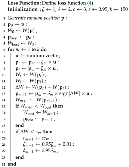
Finally, the procedure of the NABAS algorithm is shown in Algorithm 1.
| Algorithm 1: Nonlinear Activated Beetle Antennae Search (NABAS). |
 |
Remark 3.
At present, BAS and its variants have been deeply studied, and have practical applications in a wide range of fields. In [28], BAS was used to optimize the parameters of the combined motor in the power plant, which can effectively generate the optimal electric energy output. Zheng et al., discovered that BAS has good real-time performance, which provides a good solution for performance optimization control (PSC) to find the best engine performance for a specific flight mission [29]. Meanwhile, compared with commonly used machine learning methods, BAS and its variants have very good performance when applied to prediction [30,31]. Therefore, as an improved BAS, NABAS also can be applied in the same field.
4. Experiments and Verifications
Firstly, preparations of the dataset and hyperparameters are done for this problem, and the NABAS algorithm is used to solve the optimization problem (5). Then, the NABAS algorithm is compared with the other three methods, i.e., RUSBoost, logistics regression model, and SVM-FK.
4.1. Preparation
4.1.1. Preparation for Dataset
In Table 1, we enumerate the annual distribution of fraudulent companies in the dataset from 1979 to 2014. It can be seen that, compared with other years, the number of fraudulent companies accounted for a large proportion from 1991 to 2008. Considering the following four reasons, we choose the dataset from 1991 to 2008.
(1) Before 1991, not only was the number of fraudulent companies relatively low, but also some of the fraud activities were covered up. Since 1991, the nature of fraud had a significant shift in the United States. Then, the power and the law enforcement of the SEC were weakened [32].
(2) After 2008, the regulatory authorities began to reduce the law enforcement of accounting fraudulent companies, and the public resources used to detect fraudulent companies were greatly reduced. Therefore, fewer fraudulent companies were detected [32].
(3) Other technologies and relevant data we compared to our algorithm were quoted from the existing literature of other researchers, the dataset from 1991 to 2008 were used in their experiments. To increase the comparability of experiments, we used the data of the same year with them.
(4) The main contribution is to propose a universal model for the fraud detection. This model is insensitive to datasets.
In this way, the dataset from the year 1991 to 2008 is divided from Table 1. It contains 28 raw accounting variables for the training and testing of this model. In order to reduce the influence caused by the unbalanced characteristics on the experimental results, we first use SMOTE technology to oversample the minority class of fraudulent companies. Furthermore, to maintain the consistency of dataset distribution, six training sets are divided based on the year since 2001, and the datasets with an interval of two years are used as the test sets. The divided result is shown as Table 2.
Table 2.
Training data and test data.
4.1.2. Preparation for Hyperparameters
It is significant to select properly hyperparameters, which helps the detection obtain an efficient result. For this fraud detection problem, 29 variables are used as the decision variables of NABAS, which contains 28 raw accounting variables and 1 bias b. Afterward, the setting of the hyperparameters (like ) is the same as the original BAS algorithm, but is set as 2 to improve the convergence quality of the NABAS algorithm. Particularly, other hyperparameters of the model are determined by multiple experiments. For example, controls the probability of whether a company is fraudulent or not, setting to make the classification function more inclined to the category of fraud. For choosing a suitable value of , we test on the training and validation dataset of six periods. Then, we compute the average results of six experiments and show them in Table 3. Finally, by comparing the results, is chosen as the threshold because of its good performance. In addition, we try different groups of and test the performance of this model. The corresponding results are displayed in Table 4. It can be seen from Table 4 that, when the group of is (1,5), the model achieves the best performance. For readers’ convenience, all the hyperparameters of this problem are determined and separately shown in Table 5.
Table 3.
Selection of hyperparameter .
Table 4.
Selection of hyperparameter .
Table 5.
Values of hyperparameters.
4.2. Experiment Results
In this subsection, the performance of the NABAS algorithm is analyzed in detecting fraudulent companies on the given dataset from two aspects.
4.2.1. Convergence of Lost Function Value
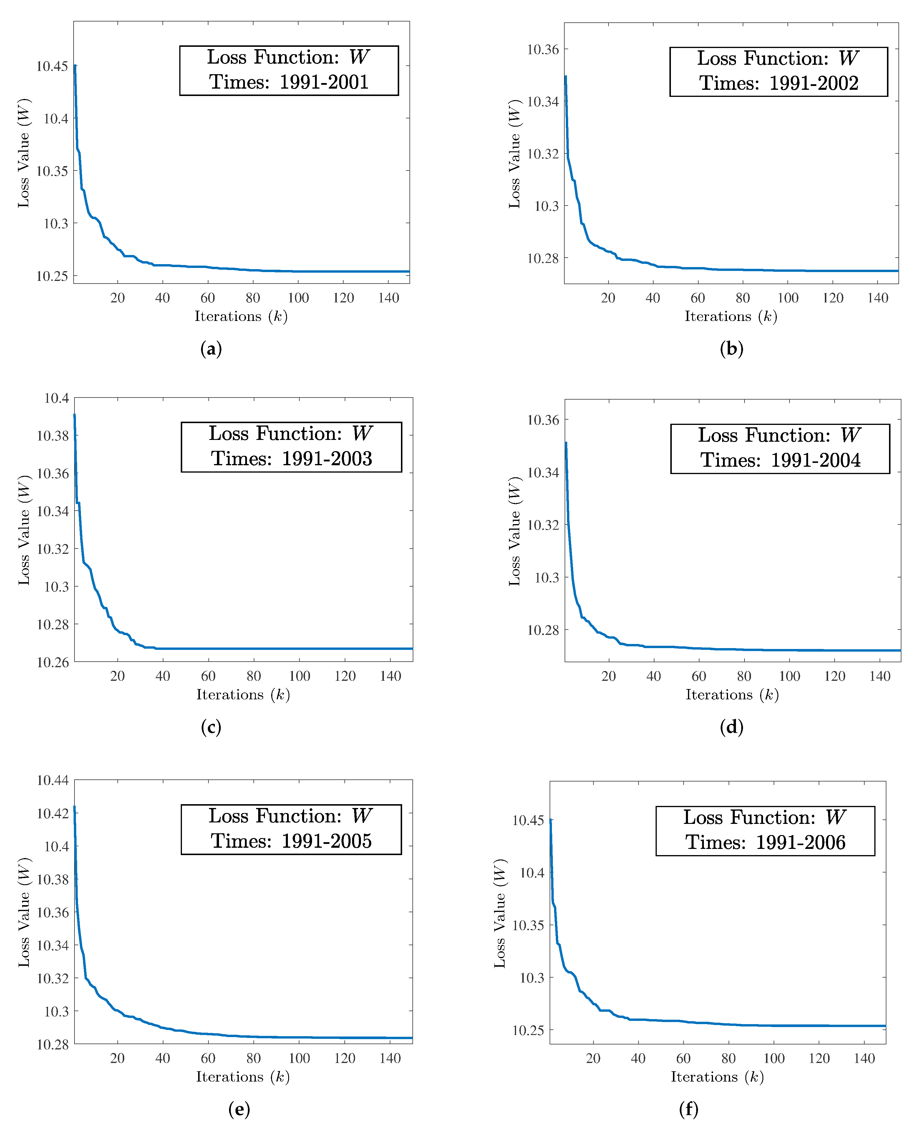
From the above subsection, the entire dataset is divided into six subsets, and the percentage of fraudulent companies varies in each subset. Then, the NABAS is used for the six subsets. In order to show the convergence results of the loss function more completely, the maximum number of iterations k of the NABAS algorithm is set to 150. All convergence results of the loss function are shown in Figure 2. As can be seen from the figures, the loss function can achieve convergence to the optimal value at a fast speed, and the number of convergence iterations is less than 100.
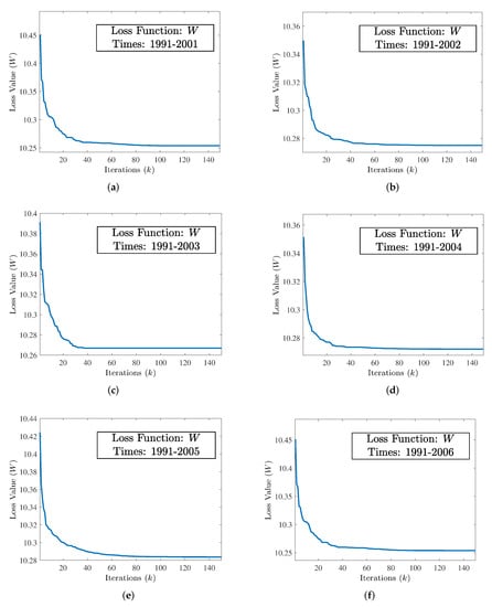
Figure 2.
The convergence of loss function (W) equipped with NABAS on six subsets of training and validation datasets from 1991–2006. (a) Convergence of NABAS on training dataset 1991–2001. (b) Convergence of NABAS on training dataset 1991–2002. (c) Convergence of NABAS on training dataset 1991–2003. (d) Convergence of NABAS on training dataset 1991–2004. (e) Convergence of NABAS on training dataset 1991–2005. (f) Convergence of NABAS on training dataset 1991–2006.
4.2.2. Yearly Comparison with RUSBoost Algorithm
The RUSBoost algorithm has been compared with Logistics and SVM-FK in [23], and the results show that RUSBoost has the best performance. Therefore, we only compare NABAS with RUSBoost by year in four evaluation indicators: accuracy, sensitivity, precision, and NDCG. The corresponding results are presented in Table 6. As shown in Table 6, for sensitivity, although NABAS is slightly inferior in the test set 2003 and the test set 2004, with the increased number of training sets and test sets, the sensitivity of NABAS is higher than RUSBoost. For other indicators, the NABAS algorithm not only has obvious advantages in accuracy, precision, and NDCG but also remains in a relatively stable range of values. The NABAS algorithm shows better and more stable prediction ability than RUSBoost. In addition, the time indicator also plays a key role in the fraud detection problem. For the same test set, the time consumed by NABAS is much less than that spent by RUSBoost. As a consequence, the NABAS algorithm has better computational efficiency than RUSBoost.
Table 6.
Comparison of NABAS and RUSBoost.
4.2.3. Comparison with Other Public Algorithms
To further verify the performance of NABAS, logistic regression model [21] and SVM-FK [22], which proposed for fraud detection in recent years, are also used to be compared with NABAS. These methods are applied to datasets from 2003 to 2008, and the average results of all indicators are depicted in Table 7. From Table 7, one can learn that the NABAS algorithm is superior to the other three methods in all indicators.
Table 7.
Comparison with other algorithms.
5. Conclusions
This paper tackles the fraud detection problem of the American publicly traded companies, and uses a dataset that was collected from SEC’s AAERs. For this problem, a fraud detection model has been proposed and transformed into an optimization problem of minimizing loss function. Meanwhile, the NABAS algorithm has been presented and employed to solve this optimization problem. Furthermore, three methods have also been used to compare with the NABAS algorithm. The experiment results show that the NABAS algorithm has better performance than other methods in all indicators. The advantage of this paper lies in the introduction of NABAS to solve the fraud detection problem and obtain higher accuracy and efficiency. However, in this study, the parameter selection is manual, which depends on repeated experiments and will incur a huge time cost. Therefore, developing an algorithm for parameter selection is a future research direction of the work.
Author Contributions
Conceptualization, B.L. and J.L.; methodology, J.L. and B.L.; software, Z.H. and X.C.; validation, Z.H. and B.L.; formal analysis, Z.H.; investigation, X.C. and Z.H.; data curation, X.C. and Z.H.; writing—original draft preparation, Z.H.; writing—review and editing, B.L. and Z.H.; visualization, Z.H.; supervision, B.L. and J.L.; project administration, B.L.; funding acquisition, J.L. All authors have read and agreed to the published version of the manuscript.
Funding
This work was supported in part by the National Natural Science Foundation of China under Grants 62066015 and 61962023, the Natural Science Foundation of Hunan Province of China under Grant 2020JJ4511, and the Research Foundation of Education Bureau of Hunan Province, China, under Grant 20A396.
Institutional Review Board Statement
Not applicable.
Informed Consent Statement
Not applicable.
Data Availability Statement
Not applicable.
Conflicts of Interest
The authors declare no conflict of interest.
References
- Alghofaili, Y.; Albattah, A.; Rassam, M.A. A Financial Fraud Detection Model Based on LSTM Deep Learning Technique. J. Appl. Secur. Res. 2020, 15, 498–516. [Google Scholar] [CrossRef]
- Delecourt, S.; Guo, L. Building a robust mobile payment fraud detection system with adversarial examples. In Proceedings of the 2019 IEEE Second International Conference on Artificial Intelligence and Knowledge Engineering (AIKE), Sardinia, Italy, 3–5 June 2019; pp. 103–106. [Google Scholar]
- Peng, L.; Lin, R. Fraud phone calls analysis based on label propagation community detection algorithm. In Proceedings of the 2018 IEEE World Congress on Services (SERVICES), San Francisco, CA, USA, 2–7 July 2018; pp. 23–24. [Google Scholar]
- Lin, T.H.; Jiang, J.R. Credit Card Fraud Detection with Autoencoder and Probabilistic Random Forest. Mathematics 2021, 9, 2683. [Google Scholar] [CrossRef]
- Ngai, E.W.; Hu, Y.; Wong, Y.H.; Chen, Y.; Sun, X. The application of data mining techniques in financial fraud detection: A classification framework and an academic review of literature. Decis. Support Syst. 2011, 50, 559–569. [Google Scholar] [CrossRef]
- Hilal, W.; Gadsden, S.A.; Yawney, J. A Review of Anomaly Detection Techniques and Applications in Financial Fraud. Expert Syst. Appl. 2021, 193, 116429. [Google Scholar] [CrossRef]
- Reurink, A. Financial fraud: A literature review. J. Econ. Surv. 2018, 32, 1292–1325. [Google Scholar] [CrossRef] [Green Version]
- Chandradeva, L.S.; Jayasooriya, I.; Aponso, A.C. Fraud Detection Solution for Monetary Transactions with Autoencoders. In Proceedings of the 2019 National Information Technology Conference (NITC), Colombo, Sri Lanka, 8–10 October 2019; pp. 31–34. [Google Scholar]
- Jain, V.; Agrawal, M.; Kumar, A. Performance Analysis of Machine Learning Algorithms in Credit Cards Fraud Detection. In Proceedings of the 2020 8th International Conference on Reliability, Infocom Technologies and Optimization (Trends and Future Directions)(ICRITO), Noida, India, 4–5 June 2020; pp. 86–88. [Google Scholar]
- Yao, L.; Wong, P.K.; Zhao, B.; Wang, Z.; Lei, L.; Wang, X.; Hu, Y. Cost-Sensitive Broad Learning System for Imbalanced Classification and Its Medical Application. Mathematics 2022, 10, 829. [Google Scholar] [CrossRef]
- Lemnaru, C.; Potolea, R. Imbalanced classification problems: Systematic study, issues and best practices. In International Conference on Enterprise Information Systems; Springer: Berlin/Heidelberg, Germany, 2011; pp. 35–50. [Google Scholar]
- Jiang, X.; Li, S. BAS: Beetle Antennae Search Algorithm for Optimization Problems. arXiv 2017, arXiv:abs/1710.10724. [Google Scholar] [CrossRef]
- Zhang, Y.; Li, S.; Xu, B. Convergence analysis of beetle antennae search algorithm and its applications. Soft Comput. 2021, 25, 10595–10608. [Google Scholar] [CrossRef]
- Katsikis, V.N.; Mourtas, S.D.; Stanimirović, P.S.; Li, S.; Cao, X. Time-varying minimum-cost portfolio insurance under transaction costs problem via Beetle Antennae Search Algorithm (BAS). Appl. Math. Comput. 2020, 385, 125453. [Google Scholar] [CrossRef]
- Katsikis, V.N.; Mourtas, S.D. Binary beetle antennae search algorithm for tangency portfolio diversification. J. Model. Optim. 2021, 13, 44–50. [Google Scholar] [CrossRef]
- Katsikis, V.N.; Mourtas, S.D. Optimal portfolio insurance under nonlinear transaction costs. J. Model. Optim. 2020, 12, 117–124. [Google Scholar] [CrossRef]
- Medvedeva, M.A.; Katsikis, V.N.; Mourtas, S.D.; Simos, T.E. Randomized time-varying knapsack problems via binary beetle antennae search algorithm: Emphasis on applications in portfolio insurance. Math. Methods Appl. Sci. 2021, 44, 2002–2012. [Google Scholar] [CrossRef]
- Mourtas, S.D.; Katsikis, V.N. V-Shaped BAS: Applications on Large Portfolios Selection Problem. In Computational Economics; Springer: Berlin/Heidelberg, Germany, 2021; pp. 1–21. [Google Scholar]
- Khan, A.T.; Cao, X.; Li, S.; Hu, B.; Katsikis, V.N. Quantum beetle antennae search: A novel technique for the constrained portfolio optimization problem. Sci. China Inf. Sci. 2021, 64, 1–14. [Google Scholar] [CrossRef]
- Khan, A.T.; Cao, X.; Li, S.; Katsikis, V.N.; Brajevic, I.; Stanimirovic, P.S. Fraud detection in publicly traded US firms using Beetle Antennae Search: A machine learning approach. Expert Syst. Appl. 2022, 191, 116148. [Google Scholar] [CrossRef]
- Dechow, P.M.; Ge, W.; Larson, C.R.; Sloan, R.G. Predicting material accounting misstatements. Contemp. Account. Res. 2011, 28, 17–82. [Google Scholar] [CrossRef]
- Cecchini, M.; Aytug, H.; Koehler, G.J.; Pathak, P. Detecting management fraud in public companies. Manag. Sci. 2010, 56, 1146–1160. [Google Scholar] [CrossRef]
- Bao, Y.; Ke, B.; Li, B.; Yu, Y.J.; Zhang, J. Detecting accounting fraud in publicly traded US firms using a machine learning approach. J. Account. Res. 2020, 58, 199–235. [Google Scholar] [CrossRef]
- Lasisi, A.; Attoh-Okine, N. Principal components analysis and track quality index: A machine learning approach. Transp. Res. Part C: Emerg. Technol. 2018, 91, 230–248. [Google Scholar] [CrossRef]
- Chawla, N.V.; Bowyer, K.W.; Hall, L.O.; Kegelmeyer, W.P. SMOTE: Synthetic minority over-sampling technique. J. Artif. Intell. Res. 2002, 16, 321–357. [Google Scholar] [CrossRef]
- Ruuska, S.; Hämäläinen, W.; Kajava, S.; Mughal, M.; Matilainen, P.; Mononen, J. Evaluation of the confusion matrix method in the validation of an automated system for measuring feeding behaviour of cattle. Behav. Process. 2018, 148, 56–62. [Google Scholar] [CrossRef] [PubMed] [Green Version]
- Wang, Y.; Wang, L.; Li, Y.; He, D.; Chen, W.; Liu, T.Y. A theoretical analysis of NDCG ranking measures. In Proceedings of the 26th Annual Conference on Learning Theory (COLT 2013), Citeseer, Princeton, NJ, USA, 12–14 June 2013; pp. 1–26. [Google Scholar]
- Ghosh, T.; Martinsen, K.; Dan, P.K. Data-Driven Beetle Antennae Search Algorithm for Electrical Power Modeling of a Combined Cycle Power Plant. In World Congress on Global Optimization; Springer: Berlin/Heidelberg, Germany, 2019; pp. 906–915. [Google Scholar]
- Zheng, Q.; Xiang, D.; Fang, J.; Wang, Y.; Zhang, H.; Hu, Z. Research on performance seeking control based on beetle antennae search algorithm. Meas. Control 2020, 53, 1440–1445. [Google Scholar] [CrossRef]
- Sun, Y.; Zhang, J.; Li, G.; Wang, Y.; Sun, J.; Jiang, C. Optimized neural network using beetle antennae search for predicting the unconfined compressive strength of jet grouting coalcretes. Int. J. Numer. Anal. Methods Geomech. 2019, 43, 801–813. [Google Scholar] [CrossRef]
- Xie, S.; Chu, X.; Zheng, M.; Liu, C. Ship predictive collision avoidance method based on an improved beetle antennae search algorithm. Ocean Eng. 2019, 192, 106542. [Google Scholar] [CrossRef]
- Rakoff, J.S. The financial crisis: Why have no high-level executives been prosecuted? N. Y. Rev. Books 2014, 9, 7. [Google Scholar]
Publisher’s Note: MDPI stays neutral with regard to jurisdictional claims in published maps and institutional affiliations. |
© 2022 by the authors. Licensee MDPI, Basel, Switzerland. This article is an open access article distributed under the terms and conditions of the Creative Commons Attribution (CC BY) license (https://creativecommons.org/licenses/by/4.0/).