Decomposition of Finitely Additive Markov Chains in Discrete Space

Abstract

In this study, we consider general Markov chains (MC) defined by a transition probability (kernel) that is finitely additive. These Markov chains were constructed by S. Ramakrishnan within the concepts and symbolism of game theory. Here, we study these MCs by using the operator approach. In our work, the state space (phase space) of the MC has any cardinality and the sigma-algebra is discrete. The construction of a phase space allows us to decompose the Markov kernel (and the Markov operators that it generates) into the sum of two components: countably additive and purely finitely additive kernels. We show that the countably additive kernel is atomic. Some properties of Markov operators with a purely finitely additive kernel and their invariant measures are also studied. A class of combined finitely additive MC and two of its subclasses are introduced, and the properties of their invariant measures are proven. Some asymptotic regularities of such MCs were revealed.

1. Introduction

In this study, classical Markov chains (MC) are interpreted as random Markov processes with discrete time (in the usual sense) in the phase space $(X,\Sigma )$, where X is some set (space) and $\Sigma$ is some sigma-algebra of subsets in X. We also consider time-homogeneous MCs. If X is an arbitrary infinite set that does not highlight any structure other than sigma-algebra $\Sigma$, then these MCs are called general.

In 1937, Kryloff and Bogoliouboff [1,2] proposed an operator-theoretical treatment of the general MC study that was then explicitly developed then by Yosida and Kakutani [3]. The essence of the treatment is that the MC is given by a transition function (probability) $P(x,E),x\in X,E\in \Sigma$, which as a kernel defines two dual integral Markov operators T and A in spaces of measurable functions and in spaces of measures, respectively.

A Markov chain is identified with an iterative sequence of probability measures $\left\{{\mu }^n\right\}$. Such sequence is generated by the second Markov operator ${\mu }^n=A{\mu }^{n-1}=A^n{\mu }^1$ with an arbitrary initial probability measure ${\mu }^1$. We use this treatment in this work.

In the classical theory of MC, the transition function (probability) $P(x,·)$ is assumed by the second argument to be a countably additive measure. At the same time, in economic game theory, developed in the 1960s by Dubbins and Savage [4], and their numerous students and followers, to also involve finitely additive probability measures in the construction of specific random processes became necessary. In particular, in [5], some constructions and investigations of finitely additive measures similar to Markov chains were presented.

Based on the work of [5], in 1981, Ramakrishnan [6] developed a new object construction in the language of strategies, thus named finitely additive Markov chains. These chains are generated by a transition function (strategy) that is finitely additive by the second argument. The phase space $(X,\Sigma )$ in [6] is a discrete set with the sigma-algebra of all its subsets. In the framework of this construction, the study in [6] contains proof of a number of non-trivial theorems, including ergodic ones, based on these specific chains properties within game theory terms. Some additional questions on this topic were also discussed in further publications by Ramakrishnan (see, e.g., [7]).

Other authors also continued to study some problems of the finitely additive Markov chains theory based on Ramakrishnan findings (see, e.g., [8]). The authors of such works actively used the special apparatus of random variables defined by finitely additive probabilities.

Zhdanok also used finitely additive measures in the study of general classical Markov chains in the works [9,10].

In this paper, we study general Markov chains generated by a transition function that is finitely additive by its second argument, as mentioned above. We consider Markov chains defined on a discrete space. However, it does not use any specific features of game theory, and a different range of problems is solved. We also do not use the apparatus of random variables.

In Section 2, we provide an operator approach for studying general Markov chains with a countably additive transition function on an arbitrary measurable space. We use and develop this construction for finitely additive transition functions.

In Section 3, a discrete topology and a discrete sigma-algebra containing all subsets of the set X are introduced into the phase space (of any cardinality) of finitely additive MCs. We study the properties of countably additive and purely finitely additive transition functions and the Markov operators generated by them in such spaces. We then prove that countably additive transition functions are atomic measures with a finitely or countable support and prove that the Markov operators of MCs with a purely finitely additive transition functions transform all finitely additive measures (including countably additive ones) into purely finitely additive measures.

The transition function of an arbitrary finitely additive MC and the Markov operators generated by it are decomposed into a countably additive component and a purely finitely additive component. Their general properties are studied.

In Section 4, we prove that, for any purely finitely additive MC, all its invariant finitely additive measures are purely finitely additive. The class of combined finitely additive MCs is also introduced here. We then prove that such MCs do not have invariant countably additive measures.

In Section 5, we consider the decomposition of a Markov sequence of measures of combined MCs into a countably additive component and a purely finitely additive component. Combined MCs have two subclasses. The first subclass is when the countably additive component of the Markov operator transforms all purely finitely additive measures into countably additive ones (condition $\left(H_1\right)$). The second subclass is when the same component transforms all purely finitely additive measures into the same ones (condition $\left(H_2\right)$). Under condition $\left(H_1\right)$, the norms of countably additive and purely finitely additive components of a Markov sequence of measures were proven to be time-stationary. Additionally, under condition $\left(H_2\right)$, the norms of countably additive components of a Markov sequence of measures were proven to converge exponentially to zero. The simple conditions $\left(G_1\right)$ and $\left(G_2\right)$ on the transition function of the MC are given, under which the “qualitative” conditions $\left(H_1\right)$ and $\left(H_2\right)$ are also satisfied. The corresponding theorems are then proven.

Examples of finitely additive MCs on a segment are considered in detail in Section 4 and Section 5 and their phase portraits are shown.

2. Definitions, Notation and Some Information

Let X be an arbitrary infinite set and $\Sigma$ be a sigma-algebra of its subsets containing all one-point subsets from X. Let $B(X,\Sigma )$ denote the Banach space of bounded $\Sigma$-measurable functions $f:X\to R$ with sup-norm.

We also consider Banach spaces of bounded measures $\mu :\Sigma \to R$, with the norm equal to the total variation of the measure $\mu$ (but one can also use the topologically equivalent sup-norm):

• $ba(X,\Sigma )$ is the space of finitely additive measures, and
• $ca(X,\Sigma )$ is the space of countably additive measures.
• If $\mu \ge 0$, then norm $\left|\right|\mu \left|\right|=\mu \left(X\right)$.

Definition 1

([11]). A finitely additive measure μ, $\mu \ge 0$, is called purely finitely additive (pure charge, pure mean) if any countably additive measure λ satisfying the condition $0\le \lambda \le \mu$ is identically zero. An alternating measure μ is called purely finitely additive if both components of its Jordan decomposition $\mu ={\mu }^{+}-{\mu }^{-}$ are purely finitely additive.

Lemma 1.

If the measure μ is purely finitely additive, then it is equal to zero on every one-point set: $\mu \left(\right\{x\left\}\right)=0,\forall x\in X$.

Proof of Lemma 1.

Take a purely finitely additive measure $\mu \ge 0$. Suppose that there is a point $x_0\in X$ such that $\mu \left(\left\{x_0\right\}\right)=\alpha >0$. We take the Dirac measure ${\delta }_{x_0}$ at the point $x_0$. Then, ${\delta }_{x_0}(X\setminus x_0)=0$ and $\alpha ·{\delta }_{x_0}\left(E\right)\le \mu \left(E\right)$ for all $E\in \Sigma$, i.e., $\alpha ·{\delta }_{x_0}\le \mu$. All Dirac measures are countably additive, and this measure $\alpha ·{\delta }_{x_0}$ is also countably additive. Therefore, the statement in Lemma 1 is true for $\mu \ge 0$. This statement is also true for any sign-alternating purely finitely additive measure. □

Obviously, a purely finitely additive measure is equal to zero on any finite set as well. The converse, generally speaking, is not true, for example, for the Lebesgue measure on the segment $[0,1]$.

Remark 1.

If the measure μ is identically zero, then it can formally be considered both countably additive and purely finitely additive.

Theorem 1

(Yosida-Hewitt decomposition, see [11]). Any finitely additive measure μ can be uniquely decomposed into the sum $\mu ={\mu }_{ca}+{\mu }_{pfa}$, where ${\mu }_{ca}$ is countably additive and ${\mu }_{pfa}$ is a purely finitely additive measure.

Bounded purely finitely additive measures also form a Banach space $pfa(X,\Sigma )$ with the same norm and $ba(X,\Sigma )=ca(X,\Sigma )\oplus pfa(X,\Sigma )$.

We denote the sets of non-negative measures:

• $V_{ba}=\{\mu \in ba(X,\Sigma ):\mu \left(X\right)\le 1\},$
• $V_{ca}=\{\mu \in ca(X,\Sigma ):\mu \left(X\right)\le 1\},$
• $V_{pfa}=\{\mu \in pfa(X,\Sigma ):\mu \left(X\right)\le 1\}.$

Measures from these sets are called probabilistic if $\mu \left(X\right)=1$.

We also denote by $S_{ba}$, $S_{ca}$, and $S_{pfa}$ the sets of all probability measures in $V_{ba}$, $V_{ca}$, and $V_{pfa}$, respectively.

Definition 2.

The classical Markov chains (MCs) on a measurable space $(X,\Sigma )$ are given by their transition function (probability kernel) $P(x,E),x\in X,E\in \Sigma$, under the usual conditions:

1. 

$0\le P(x,E)\le 1,\forall x\in X,\forall E\in \Sigma$;

2. 

$P(·,E)\in B(X,\Sigma ),\forall E\in \Sigma$;

3. 

$P(x,·)\in ca(X,\Sigma ),\forall x\in X$;

4. 

$P(x,X)=1,\forall x\in X.$

The numerical value of the function $P(x,E)$ is the probability that the system moves from the point $x\in X$ to the set $E\in \Sigma$ in one step (per unit of time).

We emphasize that the transition function of the classical Markov chain is a countably additive measure in the second argument.

We also call such transition functions countably additive kernels.

The transition function generates two Markov linear bounded positive integral operators:

• $T:B(X,\Sigma )\to B(X,\Sigma ),\left(Tf\right)\left(x\right)=Tf\left(x\right)=\underset{X}{\int }f\left(y\right)P(x,dy),$
• $\forall f\in B(X,\Sigma ),\forall x\in X;$
• $A:ca(X,\Sigma )\to ca(X,\Sigma ),\left(A\mu \right)\left(E\right)=A\mu \left(E\right)=\underset{X}{\int }P(x,E)\mu \left(dx\right),$
• $\forall \mu \in ca(X,\Sigma ),\forall E\in \Sigma .$

The operator A is isometric in the cone of non-negative measures, in particular, $A{S}_{ca}\subset S_{ca}$.

Let the initial measure be ${\mu }^1\in S_{ca}$. Then, the iterative sequence of countably additive probability measures ${\mu }^{n+1}=A{\mu }^n\in S_{ca},n\in N$ is usually identified with the Markov chain. We call $\left\{{\mu }^n\right\}$ a Markov sequence of measures.

Topologically conjugated to the space $B(X,\Sigma )$ is (isomorphically) the space of finitely additive measures: $B^{*}(X,\Sigma )=ba(X,\Sigma )$ (see, for example, [12]). In this case, the operator $T^{*}:ba(X,\Sigma )\to ba(X,\Sigma )$ serves as a topological conjugate to the operator T, which is uniquely determined by the well-known rule of integral “scalar products”:

$$⟨T^{*}\mu ,f⟩=⟨\mu ,Tf⟩,\forall f\in B(X,\Sigma ),\forall \mu \in ba(X,\Sigma ).$$

The operator $T^{*}$ is the only bounded continuation of the operator A to the space $ba(X,\Sigma )$, preserving its analytic form

$$T^{*}\mu \left(E\right)={\int }_{X}P(x,E)\mu \left(dx\right),\forall \mu \in ba(X,\Sigma ),\forall E\in \Sigma .$$

The operator $T^{*}$ has its own invariant subspace $ca(X,\Sigma )$, i.e., $T^{*}\left[ca(X,\Sigma )\right]\subset ca(X,\Sigma )$, on which it coincides with the original operator A. The operator $T^{*}$ is also isometric, and $T^{*}{S}_{ba}\subset S_{ba}$. The construction of the Markov operators T and $T^{*}$ is now functionally closed. We continue to denote the operator $T^{*}$ as A.

In such a setting, considering the Markov sequences of probabilistic finitely additive measures

$${\mu }^1\in S_{ba},{\mu }^{n+1}=A{\mu }^n\in S_{ba},n\in N,$$

and retaining the countable additivity of the transition function $P(x,·)$ by the second argument are natural.

Despite this circumstance, image $A\mu$ of a purely finitely additive measure $\mu$ can remain purely finitely additive, i.e., generally speaking,

$$A\left[ba\right(X,\Sigma \left)\right]\not\subset ca(X,\Sigma ).$$

The integral over a finitely additive measure, usually called the Radon integral, is constructed according to the same scheme as the Lebesgue integral over the Lebesgue measure. Its construction was developed in [12] and, in a more modern form, in [13]. Note that, if the original space X is countable and the measure $\mu$ is not countably additive, then the integral on X cannot be replaced by a sum (series). Such integrals have other features as well.

Definition 3.

If $A\mu =\mu$ holds for some positive finitely additive measure μ, then we call such a measure invariant for the operator A (and for the Markov chain).

An invariant probability countably additive measure is often called the stationary distribution of a Markov chain.

The question of the existence of invariant measures and their properties is one of the main questions in the theory of Markov chains.

We denote the sets of all non-zero invariant measures for the operator A as follows:

$${\Delta }_{ba}=\{\mu \in V_{ba}:\mu =A\mu \},$$

$${\Delta }_{ca}=\{\mu \in V_{ca}:\mu =A\mu \},$$

and

$${\Delta }_{pfa}=\{\mu \in V_{pfa}:\mu =A\mu \}.$$

The classical Markov chain with a countably additive transition probability may or may not have invariant countably additive probability measures, i.e., possibly ${\Delta }_{ca}=\varnothing$ (for example, for a symmetric walk on Z).

In ([14], Theorem 2.2), Šidak proved that any countably additive MC on an arbitrary measurable space $(X,\Sigma )$ with an operator extended to the space of finitely additive measures has at least one invariant finitely additive measure, i.e., always ${\Delta }_{ba}\ne \varnothing$.

In ([14], Theorem 2.5), for such MC (in the general case), Šidak established that, if a finitely additive measure $\mu$ is invariant, $A\mu =\mu$, and $\mu ={\mu }_{ca}+{\mu }_{pfa}$ is its decomposition into countably additive and purely finitely additive components, then each of them is also invariant: $A{\mu }_{ca}={\mu }_{ca}$ and $A{\mu }_{pfa}={\mu }_{pfa}$.

We now give our key definition of finitely additive MCs.

Definition 4.

A transition function of a finitely additive MC on an arbitrary (phase) measurable space $(X,\Sigma )$ is a function $P(x,E),x\in X,E\in \Sigma$, for which the conditions (1), (2), and (4) from Definition 2 and, instead of condition (3), condition $\left(3^{\prime }\right)$ are satisfied: $P(x,·)\in ba(X,\Sigma ),\forall x\in X$. We will also call such transition functions finitely additive.

We consider specific finitely additive MCs that are not countably additive in Examples 2–5 below.

The finitely additive transition function $P(x,E)$ also generates two integral operators: $T:B(X,\Sigma )\to B(X,\Sigma )$ and $A:ba(X,\Sigma )\to ba(X,\Sigma )$ in the same analytical form, with $T^{*}=A$.

The Markov operators T and $T^{*}=A$ are linear, bounded, and positive. In addition, the operator A is isometric in the cone of non-negative finitely additive measures, and $A{S}_{ba}\subset S_{ba}$. However, in this case, generally speaking, the operator A does not transform countably additive measures into the same ones, that is, $Aca(X,\Sigma )\not\subset ca(X,\Sigma )$. Finitely additive MCs are also associated with their Markov sequences of finitely additive measures $\left\{{\mu }^n\right\}$.

Remark 2.

As already noted in the Introduction, in [6], Ramakrishnan introduced the concept of finitely additive Markov chains. This definition uses a number of concepts and constructions used only in game theory. The transition function of such MCs (in our terms) in [6] was interpreted as some conditional strategy, which, as a function of sets, is finitely additive. In Definition 4 and in the following comments about Markov operators, the usual language of functional analysis (measure theory and linear operator theory) is used. Strictly comparing these completely different approaches to constructing the theory of finitely additive Markov chains is very difficult (most likely impossible). However, some analogies for individual results are easy to see.

It is natural to consider the decomposition of such transition functions (kernels) into two components: countably additive and purely finitely additive.

To define such kernels, we take as a basis Definition 2 and some information from Revuse’s book ([15], Chapter 1, §1) and transfer them to the finitely additive case.

Definition 5.

A numerical function $P(x,E)$ of two variables $x\in X$ and $E\in \Sigma$ is called a sub-Markov countably additive kernel if conditions (1), (2), and (3) from Definition 2 are satisfied.

Similarly, we introduce the terms sub-Markov and Markov kernels for the cases when the kernel $P(x,·)$ is finitely additive or purely finitely additive in the second argument for each $x\in X$.

We can say that, in this case, we replace condition (3) in Definitions 2 and 4 with the following conditions:

• ($3^{\prime }$) $P(x,·)\in ba(X,\Sigma ),\forall x\in X$, and
• ($3^{″}$) $P(x,·)\in pfa(X,\Sigma ),\forall x\in X$, respectively.

The integral operators T and A in spaces of functions and measures generated by a sub-Markov (Markov) kernel are also called sub-Markov (Markov).

The already cited Yosida–Hewitt Theorem 1 [11] on the decomposition of a finitely additive measure implies the following statement.

Proposition 1.

Let X be an infinite set and an arbitrary sigma-algebra of its subsets Σ contains all one-point sets. Any Markov finitely additive kernel $P(x,E)$ on $(X,\Sigma )$ is uniquely presented as the sum of its countably additive and purely finitely additive components: $P(x,E)=P_{ca}(x,E)+P_{pfa}(x,E),$ where $P_{ca}(x,·)\in ca(X,\Sigma ),P_{pfa}(x,·)\in pfa(X,\Sigma ),$ for all $x\in X$, $E\in \Sigma$.

Proof of Proposition 1.

The transition function of a finitely additive MC is a probability finitely additive measure $P(x,·)$ on the second argument $P(x,E),E\in \Sigma$ for each fixed $x\in X$, i.e., $P(x,·)\in ba(X,\Sigma )$, by Definition 1. Therefore, for each $x\in X$, the transition function $P(x,·)$ has a unique decomposition $P(x,·)=P_{ca}(x,·)+P_{pfa}(x,·)$ into its countably additive and finitely additive, according to Theorem 1. □

We cannot yet call the components $P_{ca}(x,·)$ and $P_{pfa}(x,·)$ sub-Markov kernels, because the $\Sigma$ -measurability of the functions $P_{ca}(·,E)$ and $P_{pfa}(·,E)$ for different $E\in \Sigma$ and for an arbitrary sigma-algebra $\Sigma$ is not guaranteed. Moreover, the original Markov kernel $P(·,E)$ is $\Sigma$ -measurable for any $E\in \Sigma$ by definition.

If the components $P_{ca}(·,E)$ or $P_{pfa}(·,E)$ are immeasurable, then no sub-Markov operators T and A are integrally expressed in terms of them.

The question of measurability with respect to the first argument of two components in the decompositions of the Markov kernel in Proposition 1 was pointed out by one of the authors of this article in their paper [9]. It was hypothesized that immeasurable decompositions exist. This problem was solved by Gutman and Sotnikov in their work [16].

They proved a number of theorems on the singularities of the decompositions of transition functions (kernels) into the sum of their countably additive and purely finitely additive components in different cases and proved that non-measurable decompositions exist, in particular, on the segment $[0,1]$ with Lebesgue sigma-algebra.

Later, Sotnikov [17] constructed a class of strongly additive transition functions in which both of their decomposition components are measurable.

In this paper, we use another possibility of ensuring the measurability of the components in the decompositions of the finitely additive Markov kernel, which serves as an introduction to the next subsection in which discrete topologies in an arbitrary MC phase space are discussed.

3. Finitely Additive Markov Kernels in Discrete Space

In the theory of Markov chains, the term “discrete” is used in different senses, and is applied to both the time parameter and the state space of the MC. We use the classical definition from functional analysis (see, for example, [18]), which is also used in some papers on the theory of MCs.

Definition 6.

A topological space $(X,\tau )$ is called discrete if all its subsets are simultaneously open and closed (clopen), that is, the topology $\tau =2^X$ is the set of all subsets of the set X.

Such a topology in X is generated by the discrete metric $d(x,y)$ equal to 1 for $x\ne y$ and equal to 0 for $x=y$. In discrete space, all points are metrically isolated. Discrete metric (and topology) can be introduced in any set X. In particular, the discrete topology can be introduced in all “principal” number sets: $N,Z,Q$, $[0,1]$, and $R=R^1$, as well as in $R^m(m\in N)$, transforming them into discrete spaces.

If a topological space is discrete, then, obviously, its Borel sigma-algebra $\mathfrak{B}=\tau =2^X$. This sigma-algebra contains all subsets of the set X. Such a sigma-algebra in X is also called discrete. We will denote it by ${\Sigma }_d$.

Ramakrishnan [6] uses a similar definition of the discrete phase space of an MC.

If the space X is discrete, then, obviously, any bounded numerical function $f:X\to R$ is measurable with respect to the discrete sigma-algebra ${\Sigma }_d$, that is, $f\in B(X,{\Sigma }_d)$. In particular, ${\Sigma }_d$ is measurable in the first argument and the components $P_{ca}(·,E)$ and $P_{pfa}(·,E)$ of the CM transition function in Proposition 1 for all $E\in \Sigma$.

Note that all numeric functions $f:X\to R$ on any discrete space $(X,{\Sigma }_d)$ are continuous in the discrete topology $\tau =2^X$.

Let us introduce the concept of a measure atom, known in different versions (we just need to use a simplified version of its definition).

Definition 7.

Let $(X,\Sigma )$ be an arbitrary measurable space and $\mu :\Sigma \to R$ be some countably additive measure. An element $x\in X$ is called an atom of the measure μ if $\mu \left(\right\{x\left\}\right)\ne 0$. If a bounded measure $\mu ,\mu \ge 0,$ has a support (set of full measure) $D\in \Sigma$, consisting of a finite or countable family of its atoms, then such a measure is called atomic (discrete). Moreover, $D=\{x_1,x_2,\cdots \}$ and $\mu \left(D\right)={\sum }_n\mu \left(\left\{x_n\right\}\right)=\mu \left(X\right)$.

The atomic measure $\mu \ge 0$ can be represented as follows

$$\mu \left(E\right)=\sum _n{\alpha }_n{\delta }_{x_n}\left(E\right),$$

where $E\in \Sigma$, ${\delta }_{x_n}$ are Dirac measures concentrated at the points $x_n$, and ${\sum }_n{\alpha }_n=\mu \left(D\right)=\mu \left(X\right)$.

Note that a countably additive measure on a nondiscrete measurable space $(X,\Sigma )$ may not have atoms, for example, the Lebesgue measure on $\left(\right[0,1],\mathfrak{B})$. Additionally, from Definition 7 and Lemma 1, any purely finitely additive measure on any measurable space has no atoms.

If the set X is countable and $\Sigma ={\Sigma }_d$, then, obviously, any bounded countably additive measure $\mu$ on $(X,{\Sigma }_d)$ is atomic.

Now, we want to find out how countably additive measures are arranged on an arbitrary discrete space $(X,{\Sigma }_d)$. In a wider formulation, this question is considered, for example, in Bourbaki ([19], Chapter III, paragraphs 1 and 2). A locally compact topological space is taken as the initial space X. Countably additive measures are defined as linear continuous functionals on the space of continuous functions. Definitions of a discrete space, a discrete (atomic) measure, and its support are given, which differ from those given above. After proving a number of propositions (theorems), in ([19], Chapter III, paragraph 2, item 5), the following statement is formulated: “on a discrete space, any measure is discrete” (here, countably additive measures).

To apply this statement in this work, we need to give precise definitions of the above and other concepts and translate them into our language. Therefore, in Theorem 2 below, we give our proof of the above statement from [19] in our definitions and refine it.

However, for this, we need one well-known and nontrivial theorem of Ulam, stated, for example, in ([20], Chapter 5, Theorems 5.6 and 5.7) and, in more detail, in ([21], Volume 1, Theorem 1.12.40, and Corollary 1.12.41). We present this theorem under the condition that the continuum hypothesis is accepted, i.e., we assume that ${\aleph }_1=c$ (continuum).

Theorem 2.

A finite countably additive measure μ defined on all subsets of the set X of cardinality ${\aleph }_1$ (c, continuum) is identically zero if it is zero for each one-point subset.

Obviously, Ulam’s theorem holds trivially for sets X with countable cardinality ${\aleph }_0$.

We continue to assume that the continuum hypothesis is true.

Remark 3.

In the books [20,21], the (extended) Ulam Theorem 2 is noted to be true and, for higher, so-called “immeasurable” cardinalities of the set X are found. Immeasurable cardinality includes all cardinalities from an ordered cardinality scale: ${\aleph }_0$, ${\aleph }_1=c$, ${\aleph }_2$, etc. There is still no example of a set with “measurable” power.

Definition 8.

A measurable space $(X,{\Sigma }_d)$ is called an arbitrary discrete space if ${\Sigma }_d=2^X$, and the set X has an arbitrary immeasurable cardinality (including from the ordered cardinality scale). In other words, we consider only discrete spaces for which the (extended) Ulam theorem is valid.

Now, let us prove the following promised theorem.

Theorem 3.

Any non-zero non-negative bounded countably additive measure $\mu :{\Sigma }_d\to R$, on an arbitrary discrete space $(X,{\Sigma }_d)$ is atomic (discrete) and has a finite or countable support $D=\{x_1,x_2,\cdots \}\subset X$, for which $\mu \left(\left\{x_n\right\}\right)={\alpha }_n>0,n\in N$, ${\sum }_n{\alpha }_n=\mu \left(D\right)=\mu \left(X\right)$, $\mu (X\setminus D)=0$.

Proof. 

For a countable set X, the assertions of the theorem are trivially fulfilled.

Now, let the set X have uncountable cardinality. Consider an arbitrary bounded non-negative countably additive measure $\mu :{\Sigma }_d\to R$ for which $0<\mu \left(X\right)=\gamma <\infty$. Because the measure $\mu$ is not identically zero, then by Theorem 2, the measure $\mu$ has at least one one-point atom $x_0\in X$ such that $\mu \left(\left\{x_0\right\}\right)={\alpha }_0>0$. We denote by D the set of all atoms of measure $\mu$. As we have shown above, $x_0\in D$ and $D\ne \varnothing$. Let us prove that the set D is finite or countable.

We split the interval $(0,\gamma ]$ of possible non-zero values of the measure $\mu$ into a countable family of disjoint intervals

$$(0,\gamma ]={\cup }_{n=1}^{\infty }(\frac{\gamma }{n+1},\frac{\gamma }{n}].$$

We denote the inverse images of these intervals as

$$D_n=\{x\in X:\mu \left(\left\{x\right\}\right)\in (\frac{\gamma }{n+1},\frac{\gamma }{n}]\},D_n\in {\Sigma }_d,n=1,2,\cdots .$$

Then, the sets $D_n$ are also pairwise disjoint and $D={\cup }_{n=1}^{\infty }{D}_n$. Therefore, since the measure $\mu$ is countably additive, then $\mu \left(D\right)={\sum }_{n=1}^{\infty }\mu \left(D_n\right)$.

By construction, for any point $x\in D_n$ performed, $\frac{\gamma }{n+1}<\mu \left(\left\{x\right\}\right)\le \frac{\gamma }{n}$, $n=1,2,\cdots$. In addition, $\mu \left(D_n\right)\le \gamma <\infty$ for all $n=1,2,\cdots$.

If any of the sets $D_n$ was infinite, then, by virtue of the inequalities for $\mu \left(\right\{x\left\}\right)$ for $x\in D_n$, it would be $\mu \left(D_n\right)=\infty .$ This contradiction implies that each set $D_n$ is finite or empty.

Therefore, the set D, as a union of a countable (or finite) family of finite sets, is countable (or finite).

By construction, $D\subset X$ and $\mu \left(D\right)\le \mu \left(X\right)$. Let us prove that $\mu \left(D\right)=\mu \left(X\right)$. Because X has uncountable cardinality and the set D is finite or countable, the set $X\setminus D\ne \varnothing$ and is also uncountable.

Suppose that $\mu \left(D\right)<\mu \left(X\right)$, i.e., $\mu (X\setminus D)>0$. By the hypothesis of the theorem, the set X is discrete. Consequently, the set $X\setminus D$ is also discrete.

The restriction ${\mu }_D$ of the measure $\mu$ from the set X to the set $X\setminus D$ also satisfies all of the requirements for the measure $\mu$ under the conditions of the theorem. Because $\mu (X\setminus D)>0$, then, again applying Ulam’s Theorem 2, we obtain that a point $y_0\in X\setminus D$ exists such that ${\mu }_D\left(\left\{y_0\right\}\right)>0$. However, then, $\mu \left(\left\{y_0\right\}\right)>0$. Therefore, $y_0\in D$ and $y_0\ne x$ for any $x\in D$. However, the set D was defined as the set of all points $x\in X$ for which $\mu \left(\right\{x\left\}\right)>0$ is satisfied. Thus, we obtain a contradiction. Therefore, $\mu \left(D\right)=\mu \left(X\right)$ and $\mu (X\setminus D)=0$.

Because D is finite or countable, we re-number all its points and obtain the last statement of the theorem. □

Surprisingly, all countably additive measures on the discrete segment $[0,1]$ are only atomic. Additionally, the Lebesgue measure does not exist on the discrete segment $[0,1]$. In 1923, Stefan Banach proved that the Lebesgue measure defined on the Borel (generated by the Euclidean topology) sigma-algebra of the segment $[0,1]$ cannot be countably additively extended to the sigma-algebra of all subsets of the segment $[0,1]$. However, it can be extended to a finitely additive measure on a discrete sigma-algebra, and infinitely many such extensions exist. This issue is discussed in many sources; see, for example, ([21], Volume 1, items 1.12.29 and 2.12.91).

Theorem 4.

A finitely additive nonnegative measure μ defined on an arbitrary discrete space $(X,{\Sigma }_d)$ is purely finitely additive if and only if the condition $\mu \left(\right\{x\left\}\right)=0$ for all $x\in X$ is fulfilled.

Proof. 

The necessity of the condition is obvious. Let us show its sufficiency. Let the condition be satisfied but the measure $\mu$ be not purely finitely additive. Then, in its decomposition $\mu ={\mu }_{ca}+{\mu }_{pfa}$ the countably additive component ${\mu }_{ca}\ne 0$. In this case, by Theorem 3, a point $x_1\in X$ exists such that ${\mu }_{ca}\left(\left\{x_1\right\}\right)>0$. From this contradiction, we can see that $\mu$ is purely finitely additive. □

Let us now return to Markov chains. Theorem 3 automatically implies the following statement.

Theorem 5.

Let a countably additive sub-Markov kernel $P(x,E)$ be given on an arbitrary discrete space $(X,{\Sigma }_d)$, and $P(x,X)>0$ for all $x\in X$. Then, for any $x\in X$, the measure $P(x,·)$ is atomic and has a finite or countable support $D\left(x\right)=\{x_1\left(x\right),x_2\left(x\right),\cdots \}$, for which

• $P(x,\left\{x_n\left(x\right)\right\})={\alpha }_n\left(x\right)>0,n\in N$,
• and ${\sum }_n{\alpha }_n\left(x\right)=P(x,D\left(x\right))=P(x,X),P(x,X\setminus D\left(x\right))=0$.

Corollary 1.

(From Theorem 4). Let a finitely additive sub-Markov kernel $P(x,E)$ be given on an arbitrary discrete space $(X,{\Sigma }_d)$. For any fixed $x_0\in X$ the measure $P(x_0,·)$ is purely finitely additive if and only if $P(x_0,\left\{y\right\})=0$ for all $y\in X$ (including the case $y=x_0$).

Example 1.

Let $X=[0,1]$ with Euclidean topology, $\Sigma =\mathfrak{B}$, be the Borel sigma-algebra and a countably additive MC given by the kernel $P(x,E)=\lambda \left(E\right)$ for all $x\in X$ and $E\in \mathfrak{B}$, where λ is the Lebesgue measure. Such a MC corresponds to a sequence of independent uniformly distributed random variables on the segment $[0,1]$. Obviously, $P(x,\{y\left\}\right)=0$ holds for all $x,y\in X$. However, the phase space $X=[0,1],\Sigma =\mathfrak{B}$ is not discrete, and Theorem 4 is not applicable.

Example 2.

Let us now take the same $X=[0,1]$ with the discrete sigma-algebra ${\Sigma }_d$. Consider a finitely additive MC defined by the kernel $P(x,E)=\eta \left(E\right)$ for all $x\in X$ and $E\in {\Sigma }_d$, where η is some purely finitely additive measure satisfying the following conditions: $\eta \ge 0$, $\eta \left(X\right)=1$ and $\eta \left(\right(0,\epsilon \left)\right)=1$ for all $\epsilon >0$. Then, obviously, the condition $P(x,\{y\left\}\right)=0$ is also satisfied for all $x,y\in X$, and Theorem 4 is applicable.

The measure $\eta$ in this example can be informally characterized as follows. It specifies a certain “random variable” that takes a value with probability 1 as close to point 0 as desired but not at point 0.

We then denote by $P^n(x,E)$ the integral convolution of the kernel $P^1(x,E)=P(x,E)$, $n=1,2,3,\dots$.

The following statement is easily proven by induction.

Corollary 2.

Let a sub-Markov purely finitely additive kernel $P(x,E)$ be given on an arbitrary discrete space $(X,{\Sigma }_d)$. Then, for all $x,y\in X$ and $n=1,2,3,\cdots$, $P^n(x,\left\{y\right\})=0$ (including the case $x=y$).

In general, the converse is not true. Here is a counter-example.

Example 3.

Let some purely finitely additive probability measure η be given on the discrete space $(X,{\Sigma }_d)$, where $X=[0,1]$. Consider on $([0,1],{\Sigma }_d)$ a finitely additive MC with the following rules for passing in one step: $P(0,\{1\left\}\right)=1,P(x,E)=\eta \left(E\right)$ for all $x\in (0,1]$ and $E\in {\Sigma }_d$. In particular, $P(x,\{y\left\}\right)=\eta \left(\right\{y\}=0$ for all $x\in (0,1]$ and $y\in [0,1]$.

Performing the integral convolution of two kernels $P(x,E)$, we obtain that $P^2(x,\left\{y\right\})=0$ for all $x\in [0,1]$ and $y\in [0,1]$. Moreover, $P(0,\{1\left\}\right)=1>0$.

As noted above in Section 2, the operator A generated by the countably additive sub-Markov kernel transforms countably additive measures into the same ones, that is, $A\left[ca\right(X,\Sigma \left)\right]\subset ca(X,\Sigma )$. This property is preserved for the particular discrete case $\Sigma =2^X$. However, if the measure $\mu \in V_{pfa}$ is purely finitely additive, then both cases are possible: $A\mu \in V_{ca}$ and $A\mu \in V_{pfa}$. However, the situation is different with a purely finitely additive kernel.

Theorem 6.

Let a purely finitely additive sub-Markov kernel $P(x,E)$ be given on an arbitrary discrete space $(X,{\Sigma }_d)$. Then, the sub-Markov operator A generated by this kernel transforms all finitely additive measures into purely finitely additive measures, that is, $A\left[ba(X,{\Sigma }_d)\right]\subset pfa(X,{\Sigma }_d)$, in particular, $A\left[ca(X,{\Sigma }_d)\right]\subset pfa(X,{\Sigma }_d)$ and $A\left[pfa(X,{\Sigma }_d)\right]\subset pfa(X,{\Sigma }_d)$.

Proof. 

Let the finitely additive measure $\mu \in V_{ba}$ and $\mu \left(X\right)>0$. We denote the measure by $\eta =A\mu$. Clearly, that the measure $\eta$ is also finitely additive.

If $\eta \left(X\right)=0$, that is, $\eta \equiv 0$ (which is possible), then it can be considered purely finitely additive (see Remark 1) and the theorem is true.

Let $\eta \left(X\right)>0$. Take its decomposition $\eta ={\eta }_{ca}+{\eta }_{pfa}$ into a countably additive component ${\eta }_{ca}$ and a purely finitely additive component ${\eta }_{pfa}$.

If ${\eta }_{ca}\left(X\right)=0$, then the measure is $\eta ={\eta }_{pfa}\in V_{pfa}$ and the theorem is proved.

Suppose that the countably additive measure ${\eta }_{ca}\left(X\right)>0$. Then, by Theorem 3, the measure ${\eta }_{ca}$ has at least one atom $a\in X$, ${\eta }_{ca}\left(\left\{a\right\}\right)=\gamma >0$. Because the measure ${\eta }_{pfa}$ is purely finitely additive, then ${\eta }_{pfa}\left(\left\{a\right\}\right)=0$.

By the hypothesis of the theorem, all kernels $P(x,·)$ are purely finitely additive for all $x\in X$. Such measures vanish on any one-point set. Therefore, $P(x,\{a\left\}\right)=0$ for all $x\in X$. Hence,

$$\gamma ={\eta }_{ca}\left(\left\{a\right\}\right)={\eta }_{ca}\left(\left\{a\right\}\right)+0={\eta }_{ca}\left(\left\{a\right\}\right)+{\eta }_{pfa}\left(\left\{a\right\}\right)=\eta \left(\left\{a\right\}\right)=A\mu \left(\left\{a\right\}\right)$$

$$={\int }_{X}P(x,\left\{a\right\})\mu \left(dx\right)={\int }_{X}0·\mu \left(dx\right)=0.$$

Thus, we obtain a contradiction. Therefore, ${\eta }_{ca}\left(X\right)=0$, and the measure $\eta ={\eta }_{pfa}=A\mu$ is purely finitely additive. □

Now, by using the discrete topology in X, we can complete Proposition 1.

Proposition 2.

Let an arbitrary discrete space $(X,{\Sigma }_d)$ be given. Any Markov finitely additive kernel $P(x,E)$ on $(X,{\Sigma }_d)$ is uniquely presented as the sum of a sub-Markov countably additive kernel $P_{ca}(x,E)$ and a sub-Markov purely finitely additive kernel $P_{pfa}(x,E)$:

$$P(x,E)=P_{ca}(x,E)+P_{pfa}(x,E),$$

where $P_{ca}(x,·)\in ca(X,{\Sigma }_d),P_{pfa}(x,·)\in pfa(X,{\Sigma }_d),$ and $P_{ca}(·,E)\in B(X,{\Sigma }_d)$, $P_{pfa}(·,E)\in B(X,{\Sigma }_d)$ for all $x\in X$ and $E\in {\Sigma }_d$.

The last inclusions, $P_{ca}(·,E)\in B(X,{\Sigma }_d)$ and $P_{pfa}(·,E)\in B(X,{\Sigma }_d)$, mean that the kernels $P_{ca}(·,E)$ and $P_{pfa}(·,E)$ are ${\Sigma }_d$-measurable in the first argument for all $E\in {\Sigma }_d$.

Proposition 2 makes it possible to introduce integral sub-Markov operators $A_{ca}$ and $A_{pfa}$ generated by the corresponding measurable subkernels. These operators act in the space of measures $A_{ca}$ and $A_{pfa}:ba(X,{\Sigma }_d)\to ba(X,{\Sigma }_d)$. They have the same analytical form as the operator A. For any $\mu \in ba(X,{\Sigma }_d)$ and $E\in \Sigma$,

$$A_{ca}\mu \left(E\right)={\int }_X{P}_{ca}(x,E)\mu \left(dx\right)$$

and

$$A_{pfa}\mu \left(E\right)={\int }_X{P}_{pfa}(x,E)\mu \left(dx\right).$$

In this case, $A=A_{ca}+A_{pfa}$.

Because integral kernels of operators are non-negative, the operators $A_{ca}$ and $A_{pfa}$ transform non-negative measures into the same ones, i.e., operators $A_{ca}$ and $A_{pfa}$ are positive. Because $0\le P_{ca}(x,E)\le P(x,E)$ and $0\le P_{pfa}(x,E)\le P(x,E)$ for all $x\in X$ and $E\in \Sigma$, the norms $\parallel A_{ca}\parallel \le \parallel A\parallel =1$ and $\parallel A_{pfa}\parallel \le \parallel A\parallel =1$, i.e., operators are bounded. Thus, both sub-Markov operators $A_{ca}$ and $A_{pfa}$ are linear, bounded (continuous), and positive, and $\parallel A_{ca}\parallel \le 1$ and $\parallel A_{pfa}\parallel \le 1$.

As we have already found out,

$$A_{ca}\left[ca(X,{\Sigma }_d)\right]\subset ca(X,{\Sigma }_d),A_{pfa}\left[ba(X,{\Sigma }_d)\right]\subset pfa(X,{\Sigma }_d).$$

Corollary 3.

The following inclusions are true for superpositions of operators $A_{ca}$ and $A_{pfa}$:

1. 

$A_{ca}·A_{ca}\left[ca(X,{\Sigma }_d)\right]\subset ca(X,{\Sigma }_d);$

2. 

$A_{pfa}·A_{pfa}\left[ba(X,{\Sigma }_d)\right]\subset pfa(X,{\Sigma }_d);$

3. 

$A_{pfa}·A_{ca}\left[ba(X,{\Sigma }_d)\right]\subset pfa(X,{\Sigma }_d).$

Remark 4.

The operators $A_{ca}$ and $A_{pfa}$, generally speaking, are non-commutative, i.e., $A_{ca}·A_{pfa}$≠$A_{pfa}·A_{ca}$.

4. Invariant Measures of Markov Operators

In the paper by Zhdanok ([9], Chapter I, §5, Theorem 5.3), the following statement was proven.

Theorem 7.

For any Markov chain with a Markov finitely additive kernel $P(x,E)$ on an arbitrary measurable space $(X,\Sigma )$, an invariant probability finitely additive measure $\mu =A\mu \in S_{ba}$ exists, that is, ${\Delta }_{ba}\ne \varnothing$.

Earlier, a similar theorem (in the language of strategies) was proven by Ramakrishnan ([6], p. 8, Theorem 2) but in the special case of a discrete phase space. In our Theorem 7 given above, no restrictions on the phase space are assumed.

Now let on an arbitrary discrete space $(X,{\Sigma }_d)$, ${\Sigma }_d=2^X$, a Markov chain with a Markov finitely additive kernel $P(x,E)$ be given. We previously identified two special “extreme” cases. The first is when the kernel $P(x,·)$ is a countably additive measure for every $x\in X$. The second is when the kernel $P(x,·)$ is a purely finitely additive measure for all $x\in X$.

The first case has already been considered in the previous paragraphs of this article and studied in a number of studies by various authors.

Consider now the second special case.

Theorem 8.

Let a Markov chain with a purely finitely additive kernel $P(x,E)$ be given on an arbitrary discrete space $(X,{\Sigma }_d)$. Then, for the Markov operator A generated by it, an invariant probabilistic finitely additive measure $\mu =A\mu \in V_{ba}$ exists and all its invariant measures are purely finitely additive, that is, ${\Delta }_{ba}={\Delta }_{pfa}\ne \varnothing$ and ${\Delta }_{ca}=\varnothing$.

Proof. 

Theorem 7 is proven for any sigma-algebra $\Sigma$ subsets of X and for any Markov finitely additive kernel. Hence, it is also true for the discrete sigma-algebra ${\Sigma }_d=2^X$ and for a purely finitely additive kernel.

Therefore, under the conditions of the present theorem, for the operator A, an invariant probabilistic finitely additive measure $\mu =A\mu$ exists, defined on the discrete space $(X,{\Sigma }_d)$.

From Theorem 6, the measure $\mu$ and all other invariant measures of the operator A are purely finitely additive. □

Definition 9.

We call a finitely additive MC on an arbitrary discrete space $(X,{\Sigma }_d)$ combined if its transition function in the decomposition

$$P(x,E)=P_{ca}(x,E)+P_{pfa}(x,E),$$

satisfies the conditions:

$$P_{ca}(x,X)=q_1,P_{pfa}(x,X)=q_2\mathit{for}\mathit{all}x\in X,$$

where $0\le q_1,q_2\le 1$, $q_1+q_2=1$.

Let the finitely additive MC be combined. Then, as shown in the comments to Proposition 2, its Markov operator A can also be represented as the sum $A=A_{ca}+A_{pfa}$ of its two components generated by the sub-Markov kernels $P_{ca}(x,E)$ and $P_{pfa}(x,E)$, wherein $\parallel A_{ca}\parallel =q_1,\parallel A_{pfa}\parallel =q_2$.

Definition 10.

A combined MC is called non-degenerate if its decomposition from Definition 9 holds for $0<q_1,q_2<1$ and degenerate if $q_1=0$ or $q_2=0$.

Above, in Section 2 and in Theorem 8, we describe the existence of invariant measures and their types for countably additive and purely finitely additive MCs. By Definition 10, they are degenerate cases of combined MCs.

Let the MC be non-degenerate. Let us take functions

$${\tilde{P}}_{ca}(x,E)=\frac{1}{q_1}{P}_{ca}(x,E),{\tilde{P}}_{pfa}(x,E)=\frac{1}{q_2}{P}_{pfa}(x,E).$$

Then, the functions ${\tilde{P}}_{ca}(x,E)$ and ${\tilde{P}}_{pfa}(x,E)$ satisfy Definition 1 and are transition functions (Markov kernels) of the corresponding Markov operators

$${\tilde{A}}_{ca}=\frac{1}{q_1}{A}_{ca},{\tilde{A}}_{pfa}=\frac{1}{q_2}{A}_{pfa}.$$

Therefore, the Markov operator A of the combined MC is a linear combination

$$A=q_1{\tilde{A}}_{ca}+q_2{\tilde{A}}_{pfa}$$

for two Markov operators ${\tilde{A}}_{ca}$ and ${\tilde{A}}_{pfa}$ (hence, the name of such MCs and operators in Definition 9 is taken).

Recall that, by Theorem 7, any, including combined, finitely additive MC has an invariant finitely additive measure.

Theorem 9.

The combined non-degenerate finitely additive MC on an arbitrary discrete space $(X,{\Sigma }_d)$ has no non-zero invariant countably additive measures, that is, ${\Delta }_{ca}=\varnothing$.

Proof. 

We carry out the proof by contradiction. Suppose that $\mu =A\mu \in S_{ca}$, i.e., the invariant measure $\mu$ is countably additive. Then,

$$\mu =A\mu =(A_{ca}+A_{pfa})\mu =A_{ca}\mu +A_{pfa}\mu ,$$

where $A_{ca}$ is countably additive, and $A_{pfa}$ are purely finitely additive components of the operator A. Then, $A_{ca}\mu$ is also a countably additive measure, and $A_{ca}\mu \left(X\right)=q_1>0$, that is, the measure $A_{ca}\mu$ is non-zero. By Theorem 6, the measure $A_{pfa}\mu$ is purely finitely additive and non-zero: $A_{pfa}\mu \left(X\right)=q_2>0$.

Consequently, the measure $\mu$ has a non-zero purely finitely additive component $A_{pfa}\mu$ and is not countably additive. The resulting contradiction proves the theorem. □

From Theorem 9, we obtain the following assertion.

Theorem 10.

Let a combined non-degenerate finitely additive MC with invariant probability finitely additive measure $\mu =A\mu \in S_{ba}$ on an arbitrary discrete space $(X,{\Sigma }_d)$ be given. Let $\mu ={\mu }_{ca}+{\mu }_{pfa}$ be its decomposition into countably additive ${\mu }_{ca}$ and purely finitely additive ${\mu }_{pfa}$ components, ${\mu }_{ca}\ne 0$, and ${\mu }_{pfa}\ne 0$.

Then, the measures ${\mu }_{ca}$ and ${\mu }_{pfa}$ are not invariant for the operator A, that is, ${\mu }_{ca}\ne A{\mu }_{ca}$ and ${\mu }_{pfa}\ne A{\mu }_{pfa}$.

Recall that by Šidak ([14], Theorem 2.5), for a MC with a countably additive kernel in a similar decomposition of the invariant measure $\mu ={\mu }_{ca}+{\mu }_{pfa}$, ${\mu }_{ca}=A{\mu }_{ca}$ and ${\mu }_{pfa}=A{\mu }_{pfa}$. The difference between such MCs and combined ones turned out to be very significant.

Let us give an example to illustrate the last two theorems.

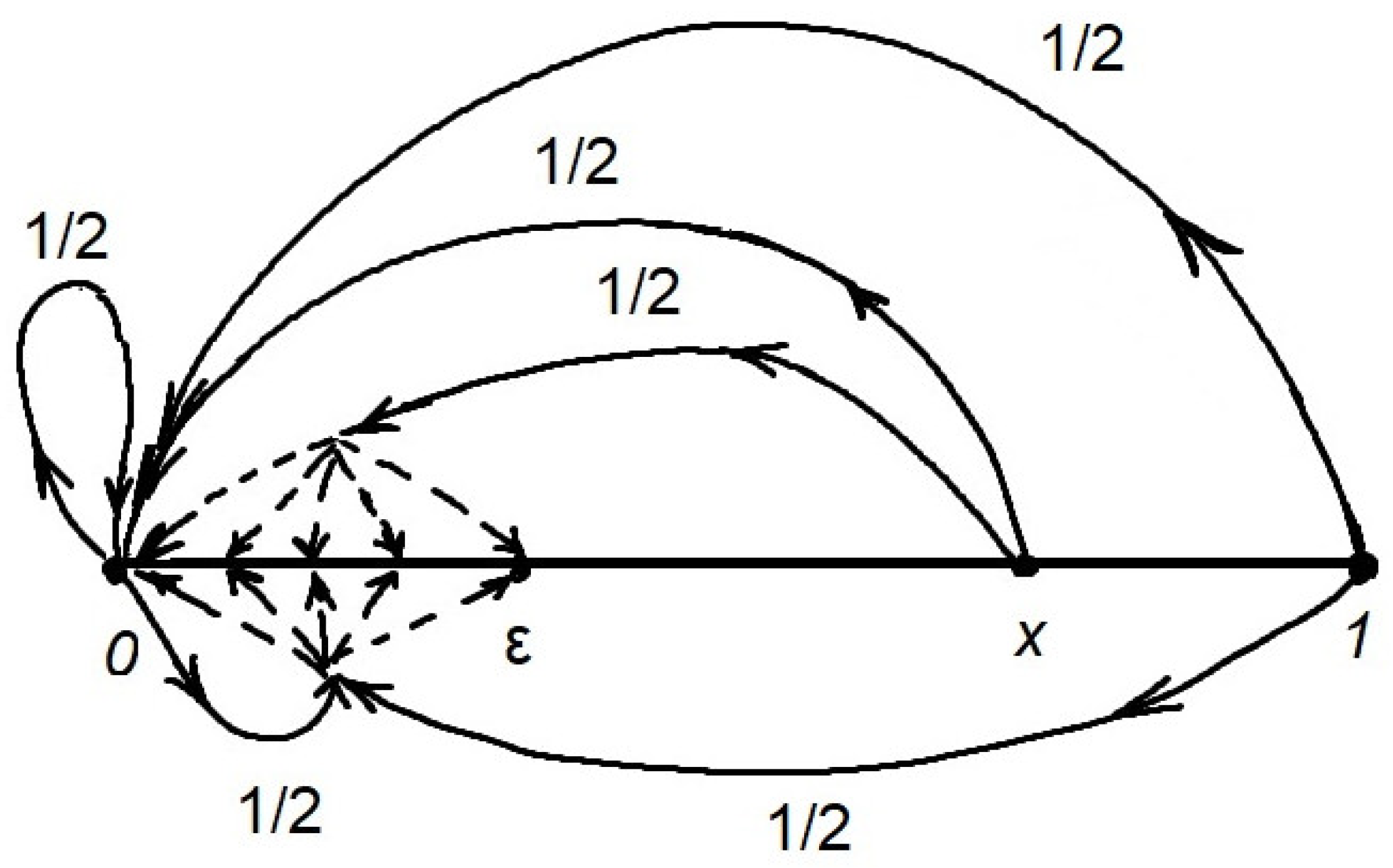
Example 4.

Consider on the segment $X=[0,1]$ with discrete sigma-algebra ${\Sigma }_d$ a combined finitely additive MC with kernel

$$P(x,E)=P_{ca}(x,E)+P_{pfa}(x,E).$$

These components are set according to the following rules:

• $P_{ca}(x,E)=\frac{1}{2}{\delta }_0\left(E\right)$ for all $x\in X$ and $E\subset X$, where ${\delta }_0$ is the Dirac at point 0;
• $P_{pfa}(x,E)=\frac{1}{2}\eta \left(E\right)$ for all $x\in X$ and $E\subset X$, where $\eta$ is some fixed purely finitely additive measure from $S_{pfa}$. For clarity, we take the measure $\eta$ from the family of purely finitely additive measures satisfying the condition $\eta \left(\right(0,\epsilon \left)\right)=1$ for any $\epsilon >0$.

Moreover, $P_{ca}(x,X)=\frac{1}{2}=q_1$ and $P_{pfa}(x,X)=\frac{1}{2}=q_2$ for all $x\in X$.

Essentially, all this means that a Markov chain in one step can move from any point $x\in X$ to point 0 with probability $\frac{1}{2}$ and to any set $E\subset X\setminus \left\{0\right\}$ with probability $\frac{1}{2}\eta \left(E\right)$. In particular, from any point $x\in X$, the system can move with probability $\frac{1}{2}$ to the open interval $(0,\epsilon )$ for every $\epsilon \in (0,1)$. The phase portrait of such a MC with an arbitrary $\epsilon \in (0,1)$ is shown in the Figure 1.

Figure 1. Phase portrait of the MC from Example 4.

Take an arbitrary (initial) finitely additive probability measure $\mu \in S_{ba}$. Then, for any $E\subset X$, the following holds:

$$A\mu \left(E\right)={\int }_{X}P(x,E)d\mu \left(x\right)={\int }_X{P}_{ca}(x,E)d\mu \left(x\right)+{\int }_X{P}_{pfa}(x,E)d\mu \left(x\right)$$

$$=\frac{1}{2}{\int }_X{\delta }_0\left(E\right)d\mu \left(x\right)+\frac{1}{2}{\int }_X\eta \left(E\right)d\mu \left(x\right)$$

$$=\frac{1}{2}{\delta }_0\left(E\right)·\mu \left(X\right)+\frac{1}{2}\eta \left(E\right)·\mu \left(X\right)=\frac{1}{2}{\delta }_0\left(E\right)+\frac{1}{2}\eta \left(E\right).$$

Hence, $A\mu =\frac{1}{2}{\delta }_0+\frac{1}{2}\eta$ for any initial measure $\mu$.

If $\mu =\frac{1}{2}{\delta }_0+\frac{1}{2}\eta$, then $A\mu =\mu$.

Obviously, this is the only invariant probabilistic finitely additive measure for a given MC.

The measures ${\mu }_{ca}=\frac{1}{2}{\delta }_0$ and ${\mu }_{pfa}=\frac{1}{2}\eta$ are non-zero components of the measure $\mu$, countably additive and purely finitely additive, respectively, and $\mu ={\mu }_{ca}+{\mu }_{pfa}$. Thus, Theorem 9 is confirmed. Then, also obvious is that $A{\mu }_{ca}=\mu \ne {\mu }_{ca}$ and $A{\mu }_{pfa}=\mu \ne {\mu }_{pfa}$. Therefore, this example also confirms Theorem 10.

In the combined non-degenerate decomposition $A=A_{ca}+A_{pfa}$ of the finitely additive operator A, its countably additive component $A_{ca}$ and the purely finitely additive component $A_{pfa}$ are equal. One might suppose that Theorem 9 would also be valid for a purely finitely additive invariant measure. However, it is not. Let us give a corresponding counterexample.

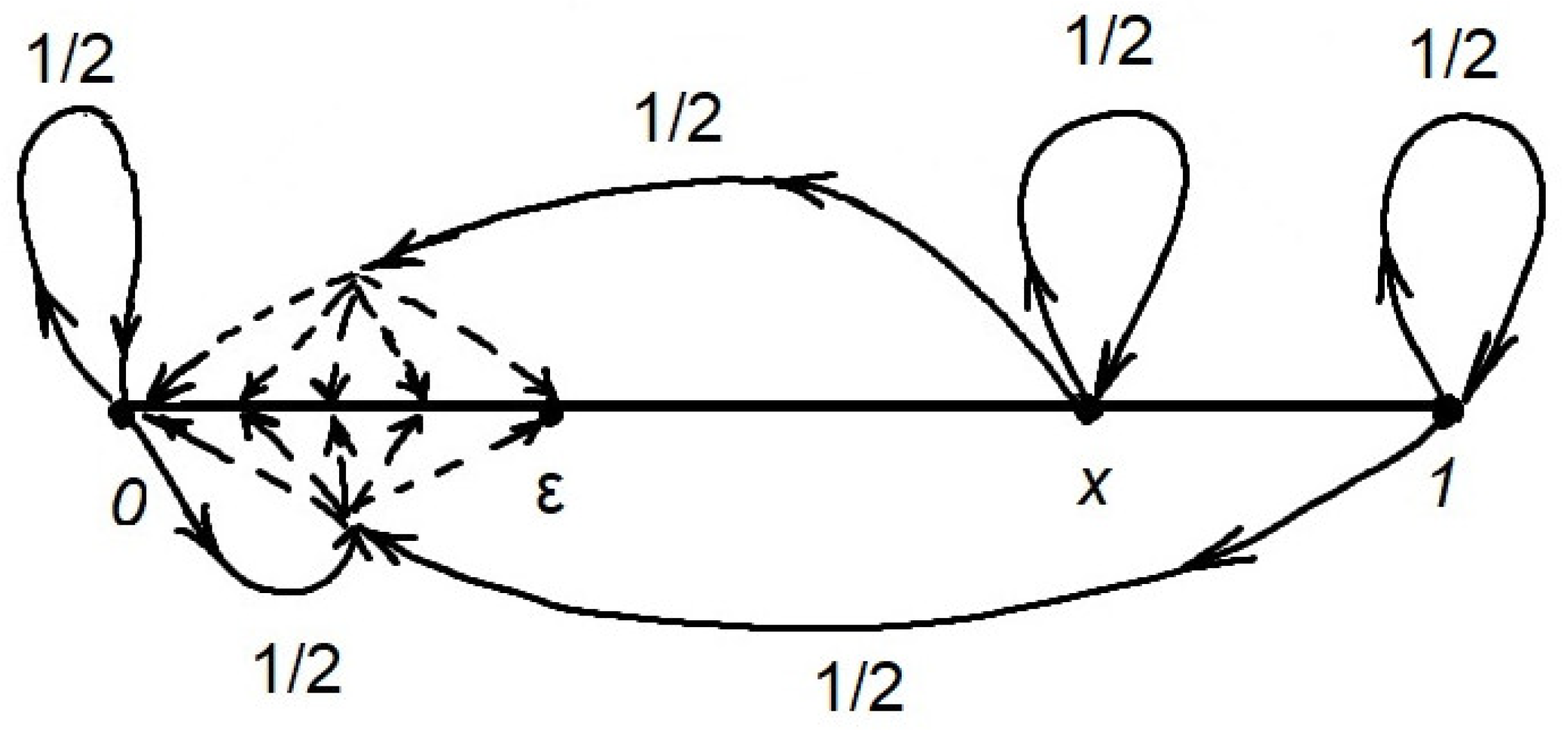
Example 5.

We consider a finitely additive combined MC on a discrete segment $X=[0,1]$ under the same conditions as in Example 4, but with a different countably additive component of its kernel:

$P_{ca}(x,E)=\frac{1}{2}{\delta }_x\left(E\right)$ for all $x\in X$ and $E\subset X$, where ${\delta }_0$ is the Dirac measure at point x.

Meaningfully, this means that, in one step, the Markov system can go from any $x\in X$ to the point x, i.e., go into itself with probability $\frac{1}{2}$ and into any set $E\subset X\setminus \left\{x\right\}$ with probability $\frac{1}{2}\eta \left(E\right)$. In particular, the probability $P_{pfa}(x,(0,\epsilon ))=\frac{1}{2}$ for any $\epsilon \in (0,1)$. The phase portrait of such a MC with an arbitrary $\epsilon \in (0,1)$ is shown in Figure 2.

Figure 2. Phase portrait of the MC from Example 5.

Obviously, this MC is a combined non-degenerate chain.

Let us perform integral transformations for an arbitrary initial probability measure $\mu \in S_{ba}$, similar to the transformations in Example 4. As a result (omitting the calculations), we have $A\mu =\frac{1}{2}\mu +\frac{1}{2}\eta$. Then, we solve the equation $\mu =A\mu$. From the last two equalities, we obtain the only solution $\mu =\eta$.

We have shown that this combined non-degenerate MC has a unique invariant finitely additive measure $\eta$, which is purely finitely additive, i.e., has no non-zero countably additive component.

5. Norms of Components in the Decomposition of a Markov Sequence of Measures and Their Asymptotic Behavior

Consider a combined non-degenerate finitely additive MC on an arbitrary discrete space $(X,{\Sigma }_d)$.

Let an arbitrary initial probability measure ${\mu }^1\in S_{ba}$, ${\mu }^1={\mu }_{ca}^1+{\mu }_{pfa}^1$, be given, and ${\mu }^{n+1}=A{\mu }^n,n\in N$ is the Markov sequence of measures generated by this initial measure. Its decomposition is

$${\mu }^{n+1}={\mu }_{ca}^{n+1}+{\mu }_{pfa}^{n+1}.$$

Remark 5.

The notation ${\mu }_{ca}^{n+1}$ can be interpreted in two ways: it can be a countably additive component of the measure ${\mu }^{n+1}$, i.e., ${\left({\mu }^{n+1}\right)}_{ca}$, or it can be $(n+1)$-th iteration of measure $\left({\mu }_{ca}^1\right)$, i.e., ${\left({\mu }_{ca}^1\right)}^{(n+1)}$. Generally speaking, these two interpretations do not coincide. Hereafter, we mean that ${\mu }_{ca}^{n+1}={\left({\mu }^{n+1}\right)}_{ca}$ and ${\mu }_{pfa}^{n+1}={\left({\mu }^{n+1}\right)}_{pfa}$, for any $n\in N$.

Because the operator A is isometric in the cone of positive measures, the norms of $\parallel {\mu }^{n+1}\parallel ={\mu }^{n+1}\left(X\right)=\parallel {\mu }^1\left(X\right)\parallel ={\mu }^1\left(X\right)=1$ for each $n\in N$.

In this section, we consider the norms of the components $\parallel {\mu }_{ca}^{n+1}\parallel$ and $\parallel {\mu }_{pfa}^{n+1}\parallel$ for $n\to \infty$.

Take the second iteration in the Markov sequence of measures ${\mu }^2=A{\mu }^1$. Let us make the appropriate transformations:

$$\begin{array}{cc}{\mu }^2={\mu }_{ca}^2+{\mu }_{pfa}^2=A{\mu }^1=(A_{ca}+A_{pfa})\hfill & ({\mu }_{ca}^1+{\mu }_{pfa}^1)\hfill \\ & =A_{ca}{\mu }_{ca}^1+A_{ca}{\mu }_{pfa}^1+A_{pfa}{\mu }_{ca}^1+A_{pfa}{\mu }_{pfa}^1.\hfill \end{array}$$

(1)

In the last four terms of the decomposition (1), the first is a countably additive measure and the third and fourth are purely finitely additive measures (see Theorem 6).

The second term $A_{ca}{\mu }_{pfa}^1$ can be a measure of any type. Consider two corresponding main cases: disjoint conditions $\left(H_1\right)$ and $\left(H_2\right)$.

$$\left(H_1\right)A_{ca}\left(V_{pfa}\right)\subset V_{ca},$$

that is, the operator $A_{ca}$ transforms all purely finitely additive measures from $V_{pfa}$ into countably additive measures. Markov chains satisfying this condition $\left(H_1\right)$ exist. Let us show that the Markov chain in Example 4 has this property. In Example 4, the Markov chain kernel has a countably additive component $P_{ca}=\frac{1}{2}{\delta }_0$.

Let $\mu$ be an arbitrary purely finitely additive measure: $\mu \in V_{pfa}$. Then, for any $E\subset X$, the following holds:

$$A_{ca}\mu \left(E\right)={\int }_X{P}_{ca}(x,E)\mu \left(dx\right)=\frac{1}{2}{\int }_X{\delta }_0\left(E\right)\mu \left(dx\right)=\frac{1}{2}{\delta }_0\left(E\right)\mu \left(X\right),$$

i.e., $A_{ca}\mu =\frac{1}{2}{\delta }_0·\mu \left(X\right)$, where the Dirac measure ${\delta }_0$ is countably additive. Therefore, condition $\left(H_1\right)$ is satisfied in Example 4.

Theorem 11.

Let condition $\left(H_1\right)$ be satisfied for a combined non-degenerate finitely additive Markov chain on an arbitrary discrete space $(X,{\Sigma }_d)$. Then, for any initial measure ${\mu }^1\in S_{ba}$ and for any $n\in N$,

$$\parallel {\mu }_{ca}^{n+1}\parallel ={\mu }_{ca}^{n+1}\left(X\right)=q_1$$

and

$$\parallel {\mu }_{pfa}^{n+1}\parallel ={\mu }_{pfa}^{n+1}\left(X\right)=q_2.$$

Proof. 

Here, we carry out the proof by induction. Let $n=1$. Then, by condition $\left(H_1\right)$, the second term $A_{ca}{\mu }_{pfa}^1$ in decomposition (1) is a countably additive measure. Therefore, due to the uniqueness of the decomposition of the Yosida–Hewitt measures, we have

$${\mu }_{ca}^2=A_{ca}{\mu }_{ca}^1+A_{ca}{\mu }_{pfa}^1=A_{ca}({\mu }_{ca}^1+{\mu }_{pfa}^1)=A_{ca}{\mu }^1.$$

From here,

$$\parallel {\mu }_{ca}^2\parallel ={\mu }_{ca}^2\left(X\right)=A_{ca}{\mu }^1\left(X\right)=q_1·{\mu }^1\left(X\right)=q_1.$$

Because

$$1=\parallel {\mu }^2\parallel ={\mu }_{ca}^2\left(X\right)+{\mu }_{pfa}^2\left(X\right)=\parallel {\mu }_{ca}^2\parallel +\parallel {\mu }_{pfa}^2\parallel ,$$

then

$$\parallel {\mu }_{pfa}^2\parallel =1-\parallel {\mu }_{ca}^2\parallel =1-q_1=q_2.$$

Thus, the statement of the theorem for $n=1$ is proven.

Suppose that the statement of the theorem is also true for some $n\in N$.

Let us make the decomposition similar to the decomposition (1) for ${\mu }^{n+1}$ and obtain the following equalities:

$$\begin{array}{cc}{\mu }^{n+1}={\mu }_{ca}^{n+1}+A{\mu }_{pfa}^{n+1}=\hfill & A{\mu }^n=(A_{ca}+A_{pfa})({\mu }_{ca}^n+{\mu }_{pfa}^n)\hfill \\ \hfill & =A_{ca}{\mu }_{ca}^n+A_{ca}{\mu }_{pfa}^n+A_{pfa}{\mu }_{ca}^n+A_{pfa}{\mu }_{pfa}^n.\hfill \end{array}$$

(2)

As in the decomposition (1), here, the first term is a countably additive measure, and the third and fourth terms are purely finitely additive measures.

By condition $\left(H_1\right)$ the second term $A_{ca}{\mu }_{pfa}^n$ in (2) is a countably additive measure. Therefore, just as for the measure ${\mu }_{ca}^2$, we obtain that ${\mu }_{ca}^{n+1}=A_{ca}{\mu }^n$. In the same way, we have that

$$\parallel {\mu }_{ca}^{n+1}\parallel ={\mu }_{ca}^{n+1}\left(X\right)=A_{ca}{\mu }^n\left(X\right)=q_1·{\mu }^n\left(X\right)=q_1$$

and

$$\parallel {\mu }_{pfa}^{n+1}\parallel ={\mu }_{pfa}^{n+1}\left(X\right)=A_{pfa}{\mu }^n\left(X\right)=q_2·{\mu }^n\left(X\right)=q_2.$$

Therefore, the statement of the theorem is true for any $n\in N$. □

Remark 6.

Norms $\parallel {\mu }_{ca}^{n+1}\parallel$ and $\parallel {\mu }_{pfa}^{n+1}\parallel$ in Theorem 11 are independent of the norms of the components of the initial measure $\parallel {\mu }_{ca}^1\parallel$ and $\parallel {\mu }_{pfa}^1\parallel$. Additionally, this is a very interesting fact.

Corollary 4.

Let the conditions of Theorem 11 be satisfied. Then, for such a Markov chain there exist invariant finitely additive measures ${\mu }^{*}=A{\mu }^{*}$, ${\mu }^{*}={\mu }_{ca}^{*}+{\mu }_{pfa}^{*}$, and for all such measures for their components, the equalities are true:

$$\parallel {\mu }_{ca}^{*}\parallel ={\mu }_{ca}^{*}\left(X\right)=q_1,\parallel {\mu }_{pfa}^{*}\parallel ={\mu }_{pfa}^{*}\left(X\right)=q_2.$$

Because Markov chains satisfying the condition $\left(H_1\right)$ are not degenerate, that is, $0<q_1,q_2<1$, they do not have invariant countably additive and invariant purely finite additive measures.

Corollary 4 clarifies our Theorem 9 under the additional condition $\left(H_1\right)$.

Remark 7.

Obviously, in Example 4, which satisfies condition $\left(H_1\right)$, the assertion of Theorem 11 is satisfied. Added to this fact is that, for any initial measure ${\mu }^1\in S_{ba}$ the following Markov measure ${\mu }^2=A{\mu }^1$ coincides with the unique invariant measure ${\mu }^2={\mu }^{*}=\frac{1}{2}{\delta }_0+\frac{1}{2}\eta$ for the given MC. It is not strictly possible to say that the MC from Example 4 “strongly converges” uniformly in the initial measures ${\mu }^1$ to the only invariant measure ${\mu }^{*}$, i.e., this MC has the best ergodic properties.

We now give the second condition $\left(H_2\right)$ related to the decomposition in (1).

$$\left(H_2\right)A_{ca}\left(V_{pfa}\right)\subset V_{pfa},$$

that is, the operator $A_{ca}$ transforms all purely finitely additive measures from $V_{pfa}$ into purely finitely additive measures. Such Markov chains exist. Let us show that the Markov chain in Example 5 has this property.

In Example 5, $P_{ca}(x,E)=\frac{1}{2}{\delta }_x\left(E\right)$ for all $x\in X$ and $E\subset X$. We take an arbitrary measure $\mu \in V_{pfa}$. Then, for all $E\subset X$, the following holds:

$$A_{ca}\mu \left(E\right)={\int }_X{P}_{ca}(x,E)\mu \left(dx\right)=\frac{1}{2}{\int }_X{\delta }_x\left(E\right)\mu \left(dx\right)=\frac{1}{2}\mu \left(E\right).$$

Thus, $A_{ca}\mu =\frac{1}{2}·\mu$, where $\mu$ is a purely finitely additive measure. Thus, condition $\left(H_2\right)$ is satisfied.

Theorem 12.

Let condition $\left(H_2\right)$ be satisfied for a combined non-degenerate finitely additive Markov chain on an arbitrary discrete space $(X,{\Sigma }_d)$. Then, for any initial finitely additive measure ${\mu }^1\in S_{ba}$, for any $n\in N$

$$\parallel {\mu }_{ca}^{n+1}\parallel ={\mu }_{ca}^{n+1}\left(X\right)=q_1^n·{\mu }_{ca}^1\left(X\right)=q_1^n·\parallel {\mu }_{ca}^1\parallel$$

and

$$\parallel {\mu }_{pfa}^{n+1}\parallel ={\mu }_{pfa}^{n+1}\left(X\right)=1-q_1^n·\parallel {\mu }_{ca}^1\parallel .$$

Proof. 

Let us return to the decomposition (1). From condition $\left(H_2\right)$, the second term $A_{ca}{\mu }_{pfa}^1$ in expansion (1) is a purely finitely additive measure. Therefore, due to the uniqueness of the Yosida–Hewitt decomposition,

$$\begin{array}{cc}{\mu }_{ca}^2=A_{ca}{\mu }_{ca}^1,\hfill & \\ \hfill & \hfill {\mu }_{pfa}^2=A_{ca}{\mu }_{pfa}^1+A_{pfa}{\mu }_{ca}^1+A_{pfa}{\mu }_{pfa}^1=A_{ca}{\mu }_{pfa}^1+A_{pfa}{\mu }^1.\end{array}$$

(3)

Find the norm of the measure ${\mu }_{ca}^2$ in equalities (3)

$$\parallel {\mu }_{ca}^2\parallel ={\mu }_{ca}^2\left(X\right)=A_{ca}{\mu }_{ca}^1\left(X\right)={\int }_X{P}_{ca}(x,X){\mu }_{ca}^1\left(dx\right)=q_1·{\mu }_{ca}^1\left(X\right)=q_1·\parallel {\mu }_{ca}^1\parallel .$$

Because $1=\parallel {\mu }^2\parallel =\parallel {\mu }_{ca}^2\parallel +\parallel {\mu }_{pfa}^2\parallel ,$ then $\parallel {\mu }_{pfa}^2\parallel =1-q_1·\parallel {\mu }_{ca}^1\parallel .$

From the equalities obtained for $n=1$$(n+1=2)$, making an assumption about the general form of the norms of the components of Markov measures is still difficult. Therefore, we now consider another case $n=2$$(n+1=3).$

Let us make transformations for the measure ${\mu }^3$, similar to transformations (1) for the measure ${\mu }^2$, relying on the condition $\left(H_2\right)$. As a result, we obtain equality for the measure

$${\mu }_{ca}^3=A_{ca}{\mu }_{ca}^2$$

and the equality for the norm of this measure

$$\parallel {\mu }_{ca}^3\parallel =q_1·{\mu }_{ca}^2\left(X\right)=q_1^2·{\mu }_{ca}^1\left(X\right)=q_1^2·\parallel {\mu }_{ca}^1\parallel .$$

From here,

$$\parallel {\mu }_{pfa}^3\parallel =1-q_1^2·\parallel {\mu }_{ca}^1\parallel .$$

Suppose now that, for arbitrary $n\in N,n\ge 2$ holds for measures ${\mu }_{ca}^n=A_{ca}{\mu }_{ca}^{n-1}$, and for the norms of these measures, we have $\parallel {\mu }_{ca}^n\parallel =q_1^{n-1}·\parallel {\mu }_{ca}^1\parallel$.

Then, (omitting transformations) we have

$${\mu }_{ca}^{n+1}=A_{ca}{\mu }_{ca}^n,$$

$$\parallel {\mu }_{ca}^{n+1}\parallel =q_1^n·\parallel {\mu }_{ca}^1\parallel ,$$

$$\parallel {\mu }_{pfa}^{n+1}\parallel =1-q_1^n·\parallel {\mu }_{ca}^1\parallel .$$

□

Remark 8.

Unlike Theorem 11, in Theorem 12, the norms of the components $\parallel {\mu }_{ca}^{n+1}\parallel$ and $\parallel {\mu }_{pfa}^{n+1}\parallel$ of the measure ${\mu }^{n+1}$ depend (linearly) on the norms of the components of the initial measure ${\mu }^1$.

Corollary 5.

Let the conditions of Theorem 12 be satisfied. Then for any finitely additive initial measure ${\mu }^1\in S_{ba}$ for the components of the Markov sequence of measures generated by it ${\mu }^{n+1}=A{\mu }^n$ as $n\to \infty$,

$$\parallel {\mu }_{ca}^n\parallel \to 0\mathrm{and}\parallel {\mu }_{pfa}^n\parallel \to 1.$$

Moreover, the convergence is uniform with respect to the initial measures ${\mu }^1\in S_{ba}$ and exponentially fast.

Corollary 6.

Let the conditions of Theorem 12 be satisfied. Then, for such a Markov chain, all of its invariant finitely additive measures (and such ones always exist, see Theorem 7) are purely finitely additive, i.e., ${\Delta }_{ba}={\Delta }_{pfa}\ne \varnothing ,{\Delta }_{ca}=\varnothing$.

This statement follows from Theorem 12 or from its Corollary 5, if we take as the initial measure ${\mu }^1$ its invariant measure ${\mu }^{*}=A{\mu }^{*}$.

Remark 9.

Let us return to the MC from Example 5. The following assertions are obtained from the properties of the MC obtained above.

Then, verifying by induction that, for any initial measure ${\mu }^1\in S_{ba}$ and for all $E\subset X$, $n\in N$,

$$|{\mu }^{n+1}\left(E\right)-\eta \left(E\right)|=\frac{1}{2^n}|{\mu }^1\left(E\right)-\eta \left(E\right)|$$

is easy. Therefore, for each $E\subset X$, $n\in N$, for the norm of a measure equal to the total variation of the measure, the following estimate is true:

$$\parallel {\mu }^{n+1}-\eta \parallel =\frac{1}{2^n}\parallel {\mu }^1-\eta \parallel \le \frac{2}{2^n}=\frac{1}{2^{n-1}}.$$

This implies that the Markov sequence of measures $\left\{{\mu }^{n+1}\right\}$ of a given MC converges strongly (in the metric topology) to a unique invariant purely finitely additive measure η. This convergence is uniform in all initial finitely additive (including countably additive) measures ${\mu }^1\in S_{ba}$. In this case, the convergence is exponentially quickly. Thus, the MC in Example 5 is ergodic.

Remark 10.

In the previous Remark 9, we talked about the limiting behavior of Markov sequences of measures, not their Cesaro means. Such an increase in the type of convergence of measures is due to the fact that the MC from Example 5 does not have cycles of measures.

The article by Zhdanok [22] was devoted to cycles of finitely additive measures. MCs with countably additive transition probability were considered with the Markov operator A extended to the space of finitely additive measures.

The conditions $\left(H_1\right)$ and $\left(H_2\right)$ are of an understandable qualitative character, but they are difficult to verify for specific MCs. Thus, finding simple analogues of these conditions in terms of the properties of the transition functions considered by the MC is desirable. We offer two such conditions. Here, we present the first of them: the $\left(G_1\right)$ condition.

$$\left(G_1\right)\left\{\begin{array}{c}\mathrm{There}\mathrm{is}\mathrm{a}\mathrm{finite}\mathrm{set}D\subset X\mathrm{such}\mathrm{that}\mathrm{for}\mathrm{all}x\in X:\hfill \\ P_{ca}(x,D)=P_{ca}(x,X)=q_1,\mathrm{which}\mathrm{is}\mathrm{equivalent}\mathrm{to}{P}_{ca}(x,X\setminus D)=0.\hfill \end{array}\right.$$

We still consider an arbitrary discrete phase space and finitely additive combined non-degenerate MCs defined on it.

Theorem 13.

Let condition $\left(G_1\right)$ be satisfied for some MC. Then,

1. 

the condition $\left(H_1\right)$ is satisfied, and

2. 

the assertion of Theorem 11 is true.

Proof. 

Let $\mu \in V_{pfa},\mu \ne 0$, i.e., the measure $\mu$ be purely finitely additive, and the measure $\eta =A_{ca}\mu$. Let condition $\left(G_1\right)$ be satisfied. Then,

$$\eta \left(D\right)=A_{ca}\mu \left(D\right)={\int }_X{P}_{ca}(x,D)\mu \left(dx\right)={\int }_X{q}_1\mu \left(dx\right)=q_1\mu \left(X\right)>0.$$

Similarly, we obtain $\eta (X\setminus D)=0$ and $\eta \left(X\right)=\eta \left(D\right)$.

The finitely additive measure $\eta =A_{ca}\mu$ is concentrated on a finite set D. Therefore, it is formally countably additive on D and on the whole space X. This means that $\eta =A_{ca}\mu \in V_{ca}$. Condition $\left(H_1\right)$ is satisfied, i.e., $\left(G_1\right)\Rightarrow \left(H_1\right)$, and the assertion of Theorem 11 is true. □

Consider one more condition $\left(G_2\right)$ on the transition function of the MC. For an arbitrary $y\in X$, we denote the set $Q_y=\{x\in X:P(x,\left\{y\right\})>0\}$.

$$\left(G_2\right)\mathrm{For}\mathrm{any}y\in X\mathrm{the}\mathrm{set}{Q}_y\mathrm{is}\mathrm{empty}\mathrm{or}\mathrm{finite}.$$

Theorem 14.

Let condition $\left(G_2\right)$ be satisfied for some MC. Then,

1. 

the condition $\left(H_2\right)$ is satisfied, and

2. 

the assertion of Theorem 12 is true.

Proof. 

Let $\mu \in V_{p}fa,\mu \ne 0$, i.e., the measure $\mu$ be purely finitely additive, and $\eta =A_{ca}\mu$. Then, for any $y\in X$, the following holds

$$\begin{array}{cc}\eta \left(\left\{y\right\}\right)=A_{ca}\mu \left(\left\{y\right\}\right)={\int }_X{P}_{ca}(x,\left\{y\right\})\hfill & \mu \left(dx\right)=\hfill \\ \hfill & {\int }_{Q_y}{P}_{ca}(x,\left\{y\right\})\mu \left(dx\right)+{\int }_{X\setminus Q_y}{P}_{ca}(x,\left\{y\right\})\mu \left(dx\right).\hfill \end{array}$$

Because a purely finitely additive measure is equal to zero on any finite set, then $\mu \left(Q_y\right)=0$, and the first integral in the expansion above is equal to zero.

By condition $\left(G_2\right)$ the function $P_{ca}(x,\left\{y\right\})$ is equal to zero for all $x\in X\setminus Q_y$. Consequently, the second integral in this expansion is equal to zero. This implies that $\eta \left(\right\{y\left\}\right)=0$. Then, the measure $\eta$ is purely finitely additive by our Theorem 4, Condition $\left(H_2\right)$ is satisfied, and the assertion of Theorem 12 is true. □

Remark 11.

Let us show that the MC in Example 4 satisfies the condition $\left(G_1\right)$. Recall that the countably additive component $P_{ca}(x,E)$ of the MC transition function in Example 4 has the following form:

$P_{ca}(x,E)=\frac{1}{2}{\delta }_0\left(E\right)$ for all $x\in X$ and $E\subset X$, where ${\delta }_0$ is the Dirac measure at point 0.

Take a finite set $D=\left\{0\right\}$. Then,

$$P_{ca}(x,D)=\frac{1}{2}{\delta }_0\left(D\right)=\frac{1}{2}=q_1,P_{ca}(x,X\setminus D)=0\mathit{for}\mathit{all}x\in X.$$

Thus, condition $\left(G_1\right)$ is fulfilled.

We showed above that the MC in Example 4 also satisfies condition $\left(H_1\right)$.

Let us now return to Example 5, in which the countably additive component of the transition function is given by the following rule: $P_{ca}(x,E)=\frac{1}{2}{\delta }_x\left(E\right)$ for all $x\in X$ and $E\subset X$, where ${\delta }_0$ is the Dirac measure at point x.

Obviously, any point $y\in X=[0,1]$ can be reached in one step only from itself with probability $\frac{1}{2}$. Hence, $Q_y=\{x\in X:P(x,\left\{y\right\})>0\}=\left\{y\right\}$. This set is finite for any $y\in X$. Thus, condition $\left(G_2\right)$ is satisfied.

Above, we directly showed (without using Theorem 14) that, in Example 5, condition $\left(H_2\right)$ also holds.

6. Conclusions

Work on the theory of finitely additive Markov chains quite naturally appeared in the general theory of random processes and in the economic game theory. Ramakrishnan’s pioneering work laid the foundations for such a theory. The main condition in this work is that the transition probability of Markov chains can only be finitely additive. However, the structures he created or used (strategies) are quite complex. They require readers to have a broad outlook in several areas of mathematics.

The authors of this article have been working on problems with using finitely additive measures to study the properties of general Markov chains for a long time. However, attention was primarily paid to classical Markov chains with countably additive transition probability. In this case, finitely additive measures appeared as a result of the extension of Markov operators from the space of countably additive measures to the space of finitely additive measures. All of these studies were carried out within the framework of the operator treatment.

We have seen that combining the problems of the theory of finitely additive Markov chains and the methods we are developing for studying general Markov chains is possible. The result is the present work. Its feature is the absence of concepts and methods of game theory and the apparatus of random variables generated by finitely additive measures. We used the language and methods of classical functional analyses available to a wider readership, and some of our results have a simple proof. However, they provide a basic platform for possible future research conducted by other authors in this direction. In particular, the ergodic properties of finitely additive Markov chains can be considered.