Estimation of Error Variance in Regularized Regression Models via Adaptive Lasso

Abstract

Estimation of error variance in a regression model is a fundamental problem in statistical modeling and inference. In high-dimensional linear models, variance estimation is a difficult problem, due to the issue of model selection. In this paper, we propose a novel approach for variance estimation that combines the reparameterization technique and the adaptive lasso, which is called the natural adaptive lasso. This method can, simultaneously, select and estimate the regression and variance parameters. Moreover, we show that the natural adaptive lasso, for regression parameters, is equivalent to the adaptive lasso. We establish the asymptotic properties of the natural adaptive lasso, for regression parameters, and derive the mean squared error bound for the variance estimator. Our theoretical results show that under appropriate regularity conditions, the natural adaptive lasso for error variance is closer to the so-called oracle estimator than some other existing methods. Finally, Monte Carlo simulations are presented, to demonstrate the superiority of the proposed method.

1. Introduction

Consider linear regression model $y={\mathit{x}}^T\mathit{\beta }+\epsilon$, where $y\in \mathbb{R}$ is the response variable, $\mathit{x}\in {\mathbb{R}}^p$ is the predictor variable, $\mathit{\beta }\in {\mathbb{R}}^p$ is the unknown regression parameter and $\epsilon \in \mathbb{R}$ is the random error satisfying $\mathit{\epsilon }\sim N(0,{\sigma }^2{\mathit{I}}_n)$. Given an $i.i.d.$ random sample ${(y_i,{\mathit{x}}_i^T)}^T\in {\mathbb{R}}^{p+1}$, $i=1,\dots ,n$, the model can be written in the matrix form as $\mathit{y}=\mathit{X}\mathit{\beta }+\mathit{\epsilon }$, where $\mathit{y}={(y_1,\dots ,y_n)}^T\in {\mathbb{R}}^n$, $\mathit{X}={[{\mathit{x}}_1,\dots ,{\mathit{x}}_n]}^T\in {\mathbb{R}}^{n\times p}$ and $\mathit{\epsilon }={({\epsilon }_1,\dots ,{\epsilon }_n)}^T\in {\mathbb{R}}^n$. In this paper, we are mainly interested in the high-dimensional sparse model, where $p\gg n$.

Regularized methods for simultaneous model selection and parameter estimation have been intensively studied in the literature, e.g., the lasso [1], smoothly clipped absolute deviation (SCAD) [2], adaptive lasso [3], bridge [4], adaptive elastic net [5], and minimax concave penalty (MCP) [6], as well as the Dantzig selector [7]. In addition, screening rules for dimension reduction are proposed, e.g., the sure independent screening method and iteratively sure independent screening method [8], lasso-based screening rules [9,10,11], etc.

However, most of these works focus on selection and estimation, with respect to regression parameters, and few studies deal with estimation of error variance, although it is a fundamental and crucial problem in statistical inference and regression analysis. In conventional linear models, the common estimator, based on residuals, plays an important role in statistical inferences and model checking. In high-dimensional models, however, variance estimation becomes a difficult problem, mainly due to two reasons. One is that the traditional residual-based methods may perform poorly or, even, fail, as, for example, the ordinary least squares method does not work when the number of covariates is greater than the sample size. The other reason is that it is difficult to select the true model, accurately, since in practice the selected model, often, contains spurious variables that are correlated with the residuals, resulting in significant underestimation of error variance (e.g., [12,13]).

Next, we provide some examples, where model error variance is involved and plays an important role.

Example 1

(Model selection). Penalization is a common approach to model selection and parameter estimation, in high-dimensional linear models. The efficiency and accuracy of such methods depend on certain tuning parameters that are chosen using some criteria, such as Mallows’s ${\mathcal{C}}_p$, Akaike’s information criterion (AIC) and the Bayesian information criterion (BIC). For example, the AIC and BIC for the lasso [14] are given by

$$\mathrm{AIC}(\mathit{X}{\widehat{\mathit{\beta }}}_{{\lambda }_n},{\sigma }^2)=\frac{{\parallel \mathit{y}-\mathit{X}{\widehat{\mathit{\beta }}}_{{\lambda }_n}\parallel }_2^2}{n{\sigma }^2}+\frac{2}{n}\mathrm{df}(\mathit{X}{\widehat{\mathit{\beta }}}_{{\lambda }_n})$$

and

$$\mathrm{BIC}(\mathit{X}{\widehat{\mathit{\beta }}}_{{\lambda }_n},{\sigma }^2)=\frac{{\parallel \mathit{y}-\mathit{X}{\widehat{\mathit{\beta }}}_{{\lambda }_n}\parallel }_2^2}{n{\sigma }^2}+\frac{log(n)}{n}\mathrm{df}(\mathit{X}{\widehat{\mathit{\beta }}}_{{\lambda }_n})$$

respectively, where ${\widehat{\mathit{\beta }}}_{{\lambda }_n}$ is the lasso estimator with tuning parameter ${\lambda }_n$ and the degrees of freedom $\mathrm{df}(\mathit{X}{\widehat{\mathit{\beta }}}_{{\lambda }_n})$ is equal to the number of non-zero elements in ${\widehat{\mathit{\beta }}}_{{\lambda }_n}$. It is easy to see that these criteria rely on error variance.

Example 2

(Confidence intervals). For a least-squares-based penalized estimator ${\widehat{\mathit{\beta }}}_{{\lambda }_n}$, let $\widehat{\mathcal{A}}$ be its index set, corresponding to non-vanishing parameters. If ${\widehat{\mathit{\beta }}}_{{\lambda }_n}$ has the oracle property, then for each $i\in \widehat{\mathcal{A}}$, the $1-\alpha$ confidence interval for ${\beta }_i$ is given by

$$[{\widehat{\beta }}_i-z_{1-\alpha /2}{c}_i{\sigma }^2,{\widehat{\beta }}_i+z_{1-\alpha /2}{c}_i{\sigma }^2],$$

where $z_{1-\alpha /2}$ is the $(1-\alpha /2)$-th quantile of the standard normal distribution and $c_i$ is the i-th diagonal element of the matrix ${({\mathit{X}}_{\widehat{\mathcal{A}}}^T{\mathit{X}}_{\widehat{\mathcal{A}}})}^{-1}$. It is clear that the above intervals depend on the variance parameter.

Example 3

(Penalized second-order least squares estimation). The second-order least squares method, in [15], extends the ordinary least squares method by, simultaneously, minimizing the first two order distances

$${\rho }_i(\mathit{\beta },{\sigma }^2)={(y_i-{\mathit{x}}_i^T\mathit{\beta },y_i^2-{({\mathit{x}}_i^T\mathit{\beta })}^2-{\sigma }^2)}^T$$

and yields the joint estimators for the regression and variance parameters. Under general conditions, the second-order least squares estimator has been shown to be, asymptotically, more efficient than the ordinary least squares estimator, if the model error has a nonzero third moment, and they are equivalent otherwise. The regularized version of this method can be used in high-dimensional models.

1.1. Literature Review

Variance estimation in high-dimensional models has attracted increasing attention in recent years. Here, we briefly review some important advances in this area. First, if the true parameter vector ${\mathit{\beta }}^{*}$ was known, then the ideal variance estimator, called the oracle estimator, is ${\sigma }_{\mathrm{oracle}}^2=(1/n){\sum }_{i=1}^n{(y_i-{\mathit{x}}_i^T{\mathit{\beta }}^{*})}^2$. Correspondingly, the estimator ${\sigma }_{\mathrm{naive}}^2={\sum }_{i=1}^n{(y_i-{\mathit{x}}_i^T\widehat{\mathit{\beta }})}^2/n$, based on some estimator $\widehat{\mathit{\beta }}$ for $\mathit{\beta }$, is called a naive estimator. Since the naive estimator is downward biased, a modified unbiased estimator is given by ${\widehat{\sigma }}^2={\sum }_{i=1}^n{(y_i-{\mathit{x}}_i^T\widehat{\mathit{\beta }})}^2/(n-\widehat{s})$, where $\widehat{s}:=\#\{i:{\widehat{\beta }}_i\ne 0\}$ is the number of nonzero elements in $\widehat{\mathit{\beta }}$. Unfortunately, when p is much larger than n, even a small change in $\widehat{s}$ will cause huge fluctuation in ${\widehat{\sigma }}^2$, if $\widehat{s}\approx n$.

To overcome this problem, Ref. [16] estimated the mean and variance parameters jointly, by maximizing a reparameterized likelihood with ${\ell }_1$ penalty:

$$({\widehat{\mathit{\varphi }}}_{{\lambda }_n},{\widehat{\rho }}_{{\lambda }_n})=arg\underset{\mathit{\varphi }\in {\mathbb{R}}^p,\rho \in {\mathbb{R}}_{+}}{min}\left\{log(\rho )+\frac{{\parallel \rho \mathit{y}-\mathit{X}\mathit{\varphi }\parallel }_2^2}{2n}+{\lambda }_n{\parallel \mathit{\varphi }\parallel }_1\right\},$$

where $\mathit{\varphi }=\mathit{\beta }/\sigma$, $\rho =1/\sigma$ and ${\mathbb{R}}_{+}=\{x\in \mathbb{R}:x>0\}$. Moreover, they proposed a generalized EM algorithm for the numerical optimization.

A refitted cross-validation (RCV) method, to derive a variance estimator, was proposed in [12], and its asymptotic properties were studied. The main idea of RCV is to attenuate the influence of irrelevant variables with high spurious correlations, via a data-splitting technique. Ref. [12], also, discussed the asymptotic properties of the lasso-based estimator ${\widehat{\sigma }}_{\mathrm{lasso}}^2={\sum }_{i=1}^n{(\mathit{y}-{\mathit{x}}_i^T{\widehat{\mathit{\beta }}}_{\mathrm{lasso}}s)}^2/(n-{\widehat{s}}_{\mathrm{lasso}})$ and SCAD-based estimator ${\widehat{\sigma }}_{\mathrm{SCAD}}^2={\sum }_{i=1}^n{(\mathit{y}-{\mathit{x}}_i^T{\widehat{\mathit{\beta }}}_{\mathrm{SCAD}})}^2/(n-{\widehat{s}}_{\mathrm{SCAD}})$, where ${\widehat{\mathit{\beta }}}_{\mathrm{lasso}}$ and ${\widehat{\mathit{\beta }}}_{\mathrm{SCAD}}$ are the least squares estimator, with ${\ell }_1$ penalty [1] and SCAD penalty [2], respectively; ${\widehat{s}}_{\mathrm{lasso}}=\#\{i:{({\widehat{\mathit{\beta }}}_{\mathrm{lasso}})}_i\ne 0\}$ and ${\widehat{s}}_{\mathrm{SCAD}}=\#\{i:{({\widehat{\mathit{\beta }}}_{\mathrm{SCAD}})}_i\ne 0\}$.

Further, a scaled lasso was proposed in [17], for simultaneous estimation of regression and variance parameters. Their model can be written as

$$({\widehat{\mathit{\beta }}}_{{\lambda }_n},{\widehat{\sigma }}_{{\lambda }_n}^2)=arg\underset{\mathit{\beta }\in {\mathbb{R}}^p,\sigma \in {\mathbb{R}}_{+}}{min}\left\{\frac{{\parallel \mathit{y}-\mathit{X}\mathit{\beta }\parallel }_2^2}{2n\sigma }+\frac{(1-a)\sigma }{2}+{\lambda }_n{\parallel \mathit{\beta }\parallel }_1\right\}.$$

Under some regularity conditions, Ref. [17] proved the oracle inequalities for prediction and their estimators.

A moment estimator for the error variance, based on the covariance matrix $\Sigma$ of the predictor variables, was studied in [18], where three cases were considered: $\Sigma =I$, estimable $\Sigma$ and non-estimable $\Sigma$. A maximum likelihood method for the normally distributed noise was developed in [19].

Moreover, Ref. [13] considered another re-parameterized likelihood, with lasso penalty

$$\begin{array}{c}\hfill ({\widehat{\mathit{\theta }}}_{{\lambda }_n},{\widehat{\varphi }}_{{\lambda }_n})\in arg\underset{\mathit{\theta }\in {\mathbb{R}}^p,\varphi \in {\mathbb{R}}_{++}}{min}\left\{-\frac{1}{2}log\varphi +\varphi \frac{{\parallel \mathit{y}\parallel }_2^2}{2n}-\frac{1}{n}{\mathit{y}}^T\mathit{X}\mathit{\theta }+\frac{{\parallel \mathit{X}\mathit{\theta }\parallel }_2^2}{2n\varphi }+{\lambda }_n\Omega (\mathit{\theta },\varphi )\right\},\end{array}$$

(1)

where ${\varphi }_{{\lambda }_n}=1/{\sigma }_{{\lambda }_n}^2$, ${\mathit{\theta }}_{{\lambda }_n}={\varphi }_{{\lambda }_n}{\mathit{\beta }}_{{\lambda }_n}$. In particular, they proposed two estimators: the natural lasso with $\Omega (\mathit{\theta },\varphi )={\parallel \mathit{\theta }\parallel }_1$ and the organic lasso with $\Omega (\mathit{\theta },\varphi )={\varphi }^{-1}{\parallel \mathit{\theta }\parallel }_1^2$.

Finally, Ref. [20] proposed a ridge-based method to estimate the error variance, under certain conditions, which is defined as follows:

$${\widehat{\sigma }}^2={\{1-n^{-1}\mathrm{tr}({\mathit{A}}_{1n})\}}^{-1}{\check{\sigma }}^2,$$

where ${\check{\sigma }}^2=n^{-1}{\mathit{y}}^T({\mathit{I}}_n-{\mathit{A}}_{1n})\mathit{y}$, ${\mathit{A}}_{1n}=n^{-1}\mathit{X}(n^{-1}{\mathit{X}}^T\mathit{X}+\eta {\mathit{I}}_p){\mathit{X}}^T$ and $\eta$ is the tuning parameter. This method performs well in low-dimensional cases, with weak signals, and it is suitable for sparse as well as non-sparse models.

1.2. Notation and Outline

Throughout the paper, let ${\mathcal{A}}_0:=\{i:{\mathit{\beta }}_i^{*}\ne 0\}$ be the index set and $s:=\#\{i:{\beta }_i^{*}\ne 0\}$ be the number of the nonzero elements of ${\mathit{\beta }}^{*}$, respectively. Given a design matrix $\mathit{X}$ and a subset $\mathcal{A}$ of $\{1,\dots ,p\}$, ${\mathit{X}}_i$ denotes the i-th column vector of $\mathit{X}$, and ${\mathit{X}}_{\mathcal{A}}$ denotes the sub-matrix, consisting of the columns with indices in $\mathcal{A}$. For vectors $\mathit{x}$, $\mathit{y}\in {\mathbb{R}}^p$, $\mathit{x}\circ \mathit{y}:={(x_1{y}_1,\dots ,x_p{y}_p)}^T$ denotes the Hadamard product. Moreover, let $1/{|\mathit{x}|\mathrm{or}|\mathit{x}|}^{-1}=(1/|x_1|,\dots ,1/|x_p{|)}^T$, $\mathrm{sgn}(\mathit{x})={(\mathrm{sgn}(x_1),\dots ,\mathrm{sgn}(x_p))}^T$, $\mathrm{sign}(\mathit{x})={(\mathrm{sign}(x_1),\dots ,\mathrm{sign}(x_p))}^T$, ${\partial \parallel \mathit{x}\parallel }_1=\partial |x_1|\times \dots \times \partial |x_p|$, where

$$\mathrm{sgn}(t)=\left\{\begin{array}{c}0,t\ne 0,\hfill \\ 1,t=0,\hfill \end{array}\right.\mathrm{sign}(t)=\left\{\begin{array}{c}1,t>0,\hfill \\ 0,t=0,\hfill \\ -1,t<0,\hfill \end{array}\right.\mathrm{and}\partial |t|=\left\{\begin{array}{c}\{1\},t>0,\hfill \\ [-1,1],t=0,\hfill \\ \{-1\},t<0.\hfill \end{array}\right.$$

The rest of this paper is organized as follows: Section 2 defines and describes the proposed natural adaptive lasso, and Section 3 gives its asymptotic properties. Section 4 deals with the numerical optimization of the proposed estimators. Monte Carlo simulation studies of finite sample properties are provided in Section 5. The conclusions and discussion are given in Section 6, while the mathematical proofs are given in Section 7.

2. Natural Adaptive Lasso (NAL)

Some researchers, e.g., Refs. [13,16], used reparameterized likelihood to jointly estimate the mean and variance parameters in high-dimensional linear models. In particular, the method of [13] has good performance, and the associated numerical computation can be converted to some simple optimization procedures. However, the natural lasso in [13] always overestimates error variance, due to the over-selection of the covariates. This motivates us to consider the more generally adaptive lasso penalty, to further improve the properties of the estimators. Consider the following adaptively weighted ${\ell }_1$-penalized likelihood

$$\begin{array}{c}\hfill ({\widehat{\mathit{\theta }}}_{{\lambda }_n},{\widehat{\varphi }}_{{\lambda }_n})\in arg\underset{\theta ,\varphi \in {\mathbb{R}}_{+}}{min}\left\{L({\mathit{\theta }}_{{\lambda }_n},{\varphi }_{{\lambda }_n})+{\lambda }_n{\parallel \mathit{w}\circ \mathit{\theta }\parallel }_1\right\},\end{array}$$

(2)

where $L({\mathit{\theta }}_{{\lambda }_n},{\varphi }_{{\lambda }_n})$ is the reparameterized likelihood as (1), ${\lambda }_n$ is the tuning parameter and $\mathit{w}:={(w_1,\dots ,w_p)}^T$ is the adaptive weight vector. Given a solution $({\widehat{\mathit{\theta }}}_{{\lambda }_n},{\widehat{\varphi }}_{{\lambda }_n})$ of problem (2), the natural adaptive lasso estimators (NALE) for $\mathit{\beta }$ and ${\sigma }^2$ are given by

$${\widehat{\mathit{\beta }}}_{{\lambda }_n}=\frac{{\widehat{\mathit{\theta }}}_{{\lambda }_n}}{{\widehat{\varphi }}_{{\lambda }_n}},{\widehat{\sigma }}_{{\lambda }_n}^2=\frac{1}{{\widehat{\varphi }}_{{\lambda }_n}}.$$

(3)

It is easy to see that, when $\mathit{w}=\mathbf{1}$, the NALE reduces to the natural lasso estimator (NLE) of [13].

Note that the quality of the NALE depends on the weight vector $\mathit{w}$. It follows from Proposition 1 in Section 3, that the weight $\mathit{w}$ in problem (2) plays the same role as in the adaptive lasso estimation of the regression coefficients only, which solves the following convex optimization problem:

$$\begin{array}{c}\hfill {\widehat{\mathit{\beta }}}_{\mathrm{ada}}=arg\underset{\mathit{\beta }\in {\mathbb{R}}^p}{min}\left\{\frac{1}{n}{\parallel \mathit{y}-\mathit{X}\mathit{\beta }\parallel }_2^2+2{\lambda }_n{\parallel \mathit{w}\circ \mathit{\beta }\parallel }_1\right\},\end{array}$$

(4)

where the weight $\mathit{w}$ depends on the initial estimator ${\tilde{\mathit{\beta }}}^{\mathrm{ini}}$. As indicated by [3], any root-n consistent estimator can be used as the initial estimator for $\mathit{\beta }$. For example, the least squares estimator ${\widehat{\mathit{\beta }}}_{\mathrm{ols}}:={({\mathit{X}}^T\mathit{X})}^{-1}{\mathit{X}}^T\mathit{y}$ can be used, and the weight vector is calculated as $\mathit{w}=1/|{\widehat{\mathit{\beta }}}_{\mathrm{ols}}{|}^{\gamma }$, $\gamma >0$. Ref. [4] discusses the selection of the initial estimators in linear models, with $logp=O(n^a)$ for some $a\in (0,1)$. They show that their marginal regression estimator can be used in the adaptive lasso, to yield the desirable selection and estimation properties. In addition, the weight $\mathit{w}$ in adaptive elastic-net [5], for moderate dimensional models ($logp=O(logn)$), can be constructed as $\mathit{w}=1/|{\widehat{\mathit{\beta }}}_{\mathrm{net}}+(1/n)\mathrm{sgn}({\widehat{\mathit{\beta }}}_{\mathrm{net}}){|}^{\gamma }$, $\gamma >0$, where ${\widehat{\mathit{\beta }}}_{\mathrm{net}}$ is the elastic-net estimator. In this paper, we use the following two-step procedure to calculate the weight vector.

Step 1: Solve the lasso problem to obtain the NLE ${\widehat{\mathit{\beta }}}_{\mathrm{lasso}}$, which is used as the initial estimator ${\tilde{\mathit{\beta }}}^{\mathrm{ini}}$.

Step 2: Set $\mathit{w}$ with $w_j=p_{{\lambda }_n}^{\prime }(|{\tilde{\beta }}_j^{\mathrm{ini}}|)$, where $j=1,\dots ,p$ and $p_{{\lambda }_n}$ is a folded-concave penalty function (such as SCAD, MCP or bridge).

Remark 1.

From [7,21,22], under some regularity conditions, the lasso is consistent with a near-oracle rate $\sqrt{slogp/n}$ and has the sure-screening property, i.e.,

$$\parallel {\widehat{\mathit{\beta }}}_{\mathrm{lasso}}-{\mathit{\beta }}^{*}{\parallel }_2\le O(\sqrt{slog(p)/n}),\mathrm{supp}({\widehat{\mathit{\beta }}}_{\mathrm{lasso}})\supseteq \mathrm{supp}({\mathit{\beta }}^{*}).$$

Further, based on the order of the bias of the lasso, under suitable conditions for the minimum signal strength (dee the first part of Condition 4 in Section 7) and the choice of tuning parameter, ${\mathit{w}}_{{\mathcal{A}}_0}$ will be close, or even equal, to zero vector, when n is sufficiently larger, if a folded-concave penalty, such as SCAD, is used. These properties play an important role in some of the conclusions that follow.

3. Asymptotic Properties

In this section, we, first, establish the relationship between the NALE and the adaptive lasso, then analyze the asymptotic properties of the NALE for ${\sigma }^2$.

Proposition 1.

The NALE estimator $({\widehat{\mathit{\beta }}}_{{\lambda }_n},{\widehat{\sigma }}_{{\lambda }_n}^2)$, defined in (3), where $({\widehat{\mathit{\theta }}}_{{\lambda }_n},{\widehat{\varphi }}_{{\lambda }_n})$ is a solution of (2), satisfies the following properties:

(i) 

${\widehat{\mathit{\beta }}}_{{\lambda }_n}$ is a solution of the adaptive lasso (4);

(ii) 

${\widehat{\sigma }}_{{\lambda }_n}^2$ is the optimal value, of the objective function of the adaptive lasso (4). Furthermore, we have ${\widehat{\sigma }}_{{\lambda }_n}^2=n^{-1}{(\parallel \mathit{y}\parallel }_2^2-\parallel \mathit{X}{\widehat{\mathit{\beta }}}_{{\lambda }_n}{\parallel }_2^2)$.

The results of Proposition 1 are instrumental in the derivation of the other theoretical results in this paper. Moreover, they, also, provide a method for calculating the NALE for $\mathit{\beta }$ and ${\sigma }^2$. It is well known that the adaptive lasso (4) is a convex optimization, and many existing optimization tools can be used to compute this problem.

Note that, since

$$\begin{array}{ccc}\hfill {\widehat{\sigma }}_{{\lambda }_n}^2& =& \frac{1}{n}\parallel \mathit{y}-\mathit{X}{\widehat{\mathit{\beta }}}_{{\lambda }_n}{\parallel }_2^2+2{\lambda }_n{\parallel \mathit{w}\circ {\widehat{\mathit{\beta }}}_{{\lambda }_n}\parallel }_1\hfill \\ & =& {\widehat{\sigma }}_{\mathrm{naive}}^2({\widehat{\mathit{\beta }}}_{{\lambda }_n})+2{\lambda }_n{\parallel \mathit{w}\circ {\widehat{\mathit{\beta }}}_{{\lambda }_n}\parallel }_1\hfill \end{array}$$

(5)

and $\parallel \mathit{w}\circ {\widehat{\mathit{\beta }}}_{{\lambda }_n}{\parallel }_1={\parallel {\mathit{w}}_{{\mathcal{A}}_0}\circ {\widehat{\mathit{\beta }}}_{{\mathcal{A}}_0}\parallel }_1$ will be close or even equal to zero, for suitably chosen $\mathit{w}$, the NALE for ${\sigma }^2$ will be close to the naive estimator, if ${\lambda }_n\to 0$. As mentioned before, the naive estimator for ${\sigma }^2$, based on the adaptive lasso estimator ${\widehat{\mathit{\beta }}}_{{\lambda }_n}$, may work well when non-zero variables are selected, accurately. However, when more irrelevant variables are selected, the value of the penalty term will not be close to 0 in the finite sample, so that the naive estimator for ${\sigma }^2$ will, always, underestimate the true error variance. In this case, the penalty term will mitigate the difference between the naive estimator and the true variance. Although the form of the natural lasso estimator of [13] is similar to (5), their method often tends to over-select predictors, due to the use of a lasso penalty. In addition, the value of the penalty term in [13] remains large because it is not controlled by the weight vector. These facts explain why the natural lasso estimator for ${\sigma }^2$ tends to be larger than the true error variance in the simulation studies, in [13].

Next, we establish a key inequality for the NALE for ${\sigma }^2$.

Lemma 1.

If ${\lambda }_n\ge \frac{1}{n}{\parallel {\mathit{X}}^T\mathit{\epsilon }\parallel }_{\infty }$, then

$$|{\widehat{\sigma }}_{{\lambda }_n}^2-\frac{1}{n}{\parallel \mathit{\epsilon }\parallel }_2^2|\le 2{\lambda }_{n}max\left\{\parallel \mathit{w}\circ {\mathit{\beta }}^{*}{\parallel }_1,{\parallel {\widehat{\mathit{\beta }}}_{{\lambda }_n}-{\mathit{\beta }}^{*}\parallel }_1\right\}.$$

The above inequality is deterministic, in that it does not rely on any statistical assumptions for $\mathit{X}$ and $\mathit{\epsilon }$. Unlike Lemma 1 in [13], the proof of this result uses the fact that any vector $\mathit{\beta }$ provides an upper bound on ${\widehat{\sigma }}_{{\lambda }_n}^2$ and the convexity of the loss function. In addition, if $\mathit{w}={(1,\dots ,1)}^T$ and $O(\parallel {\widehat{\mathit{\beta }}}_{{\lambda }_n}-{\mathit{\beta }}^{*}{\parallel }_1)\le O(\parallel {\mathit{\beta }}^{*}{\parallel }_1)$, Lemma 1 reduces to Lemma 1 in [13]. If $\mathit{w}$ is close or equal to zero, and $O(\parallel {\widehat{\mathit{\beta }}}_{{\lambda }_n}-{\mathit{\beta }}^{*}{\parallel }_1)\le O(\parallel {\mathit{\beta }}^{*}{\parallel }_1)$, then the bound on the right-hand side of the inequality in Lemma 1 is lower than that for the natural lasso and organic lasso in [13].

3.1. Adaptive Lasso

It follows, from Lemma 1, that the error bound of the NALE for ${\sigma }^2$ is controlled by the convergence rate of the adaptive-lasso estimator ${\widehat{\mathit{\beta }}}_{{\lambda }_n}$. Therefore, it is necessary to establish the asymptotic properties for ${\widehat{\mathit{\beta }}}_{{\lambda }_n}$. The results in this subsection are similar to that in [23]. All regularity conditions and proofs are given in Section 7.

Theorem 1.

Suppose Conditions 1–3 hold. Assume that

$$\underset{i\in {\mathcal{A}}_0^c}{min}{w}_i^{*}>C_1^{-1},{\lambda }_n=4C_1\sigma \sqrt{(2logp+2L)/n}$$

and $s(log(p)+L)/n\to 0$, where $C_1$ is some positive constant and $L>0$. Then, with probability at least $1-e^{-L}$, there exists unique minimizer ${\widehat{\mathit{\beta }}}_{{\lambda }_n}=({\widehat{\mathit{\beta }}}_{{\mathcal{A}}_0}^T,{\widehat{\mathit{\beta }}}_{{\mathcal{A}}_0^c}^T)$ of problem (4), such that ${\widehat{\mathit{\beta }}}_{{\mathcal{A}}_0^c}=\mathbf{0}$ and $\parallel {\widehat{\mathit{\beta }}}_{{\lambda }_n}-{\mathit{\beta }}^{*}{\parallel }_2\le a_n$, where

$$a_n=C_4(\sqrt{s(2logp+2L)/n}+2{\lambda }_n(\parallel {\mathit{w}}_{{\mathcal{A}}_0}^{*}{\parallel }_2+C_2{C}_3\sqrt{s(logp)/n}))$$

with some constant $C_4>0$, $C_2$ and $C_3$ are defined in the regularity conditions.

It follows from inequality (18) that the extra term ${\lambda }_n\sqrt{s(logp)/n}$ in $a_n$ is due to the bias of the initial estimator ${\tilde{\mathit{\beta }}}^{\mathrm{ini}}$. When ${\lambda }_n$ tends to zero, the order of the extra term is $o(\sqrt{s(logp)/n})$. Thus, under some general conditions, the convergence rate of ${\widehat{\mathit{\beta }}}_{{\lambda }_n}$ is $O(\sqrt{s(log(p)+L)/n})$. Usually, the order of L is $O(logp)$.

We, now, present the asymptotic normality of the adaptive-lasso estimator ${\widehat{\mathit{\beta }}}_{{\lambda }_n}$.

Theorem 2.

Assume that conditions of Theorem 1 hold. Let $s_n^2=(1/n){\sigma }^2{\mathit{\alpha }}_n^T{\mathit{X}}_{{\mathcal{A}}_0}^T{\mathit{X}}_{{\mathcal{A}}_0}{\mathit{\alpha }}_n$ for any ${\mathit{\alpha }}_n\in {\mathbb{R}}^s$ satisfying ${\parallel \mathit{\alpha }\parallel }_2\le 1$. Then, under Conditions 1–4, with probability at least $1-e^{-L}$, the minimizer ${\widehat{\mathit{\beta }}}_{{\lambda }_n}$ in Theorem 1 satisfies

$$\begin{array}{c}\hfill n^{\frac{1}{2}}{s}_n^{-1}{\mathit{\alpha }}_n^T\left[({\widehat{\mathit{\beta }}}_{{\mathcal{A}}_0}-{\mathit{\beta }}_{{\mathcal{A}}_0}^{*})+n{\mathit{\alpha }}_n^T{({\mathit{X}}_{{\mathcal{A}}_0}^T{\mathit{X}}_{{\mathcal{A}}_0})}^{-1}{\lambda }_n{\mathit{w}}_{{\mathcal{A}}_0}^{*}\circ {\mathit{g}}_{{\mathcal{A}}_0}^{*}\right]\\ \hfill =n^{1/2}{s}_n^{-1}{\mathit{\alpha }}_n^T{({\mathit{X}}_{{\mathcal{A}}_0}^T{\mathit{X}}_{{\mathcal{A}}_0})}^{-1}{\mathit{X}}_{{\mathcal{A}}_0}^T\mathit{\epsilon }+o_p(1)\stackrel{\mathcal{D}}{\to }N(0,1),\end{array}$$

where $g_{{\mathcal{A}}_0}^{*}\in \partial {\parallel {\mathit{\beta }}_{{\mathcal{A}}_0}^{*}\parallel }_1$.

The result of Theorem 2 is consistent with the asymptotic normality, for the bridge estimator of $\mathit{\beta }$ in [4]. The only difference is in the form of the penalty function.

Next, we consider the convergence performance of the specific adaptive-lasso estimator ${\widehat{\mathit{\beta }}}_{{\lambda }_n}$, with a weight vector decided by the SCAD penalty [23], which is defined by

$$p_{{\lambda }_n}^{\prime }(|t|)=\mathbf{1}\{|t|\le {\lambda }_n^{\mathrm{SCAD}}\}+\frac{(a{\lambda }_n^{\mathrm{SCAD}}-{|t|)}_{+}}{(a-1){\lambda }_n^{\mathrm{SCAD}}}\mathbf{1}\{|t|>{\lambda }_n^{\mathrm{SCAD}}\},$$

where $a>2$ is a given constant and ${(·)}_{+}:=max\{0,·\}$. Usually, the order of ${\lambda }_n^{\mathrm{SCAD}}$ is $O(\sqrt{s(logp+L)/n})$. By definition, it holds $w_{{\mathcal{A}}_0}^{*}=\mathbf{0}$, and Condition 4 is satisfied when ${min}_{i\in {\mathcal{A}}_0}|{\beta }_i^{*}|\ge 2a{\lambda }_n^{\mathrm{SCAD}}$. Thus, we have the following result.

Corollary 1.

Assume that the conditions of Theorem 1 hold. Then, under Conditions 1–4, with probability at least $1-e^{-L}$, there exists unique minimizer ${\widehat{\mathit{\beta }}}_{{\lambda }_n}=({\widehat{\mathit{\beta }}}_{{\mathcal{A}}_0}^T,{\widehat{\mathit{\beta }}}_{{\mathcal{A}}_0^c}^T)$ of problem (4), such that

$$\begin{array}{c}\parallel {\widehat{\mathit{\beta }}}_{{\lambda }_n}-{\mathit{\beta }}^{*}{\parallel }_2\le O(\sqrt{s(logp+L)/n}),\hfill \\ \mathrm{sgn}({\widehat{\mathit{\beta }}}_{{\mathcal{A}}_0})=\mathrm{sgn}({\mathit{\beta }}_{{\mathcal{A}}_0}^{*})and{\widehat{\mathit{\beta }}}_{{\mathcal{A}}_0^c}=\mathbf{0}.\hfill \end{array}$$

Furthermore, ${\widehat{\mathit{\beta }}}_{{\lambda }_n}$ satisfies

$$n^{\frac{1}{2}}{s}_n^{-1}{\mathit{\alpha }}_n^T({\widehat{\mathit{\beta }}}_{{\mathcal{A}}_0}-{\mathit{\beta }}_{{\mathcal{A}}_0}^{*})=n^{1/2}{\mathit{\alpha }}_n^T{({\mathit{X}}_{{\mathcal{A}}_0}^T{\mathit{X}}_{{\mathcal{A}}_0})}^{-1}{\mathit{X}}_{{\mathcal{A}}_0}^T\mathit{\epsilon }\stackrel{\mathcal{D}}{\to }N(0,1),$$

where $s_n^2=(1/n){\sigma }^2{\mathit{\alpha }}_n^T{\mathit{X}}_{{\mathcal{A}}_0}^T{\mathit{X}}_{{\mathcal{A}}_0}{\mathit{\alpha }}_n$ for any ${\mathit{\alpha }}_n\in {\mathbb{R}}^s$ satisfying $\parallel {\mathit{\alpha }}_n{\parallel }_2\le 1$.

The rate of convergence of the estimators in Theorem 1 and Corollary 1 is controlled by the distribution of random error and predictor matrix. Moreover, these results can be generalized for other situations, where random error follows sub-Gaussian or sub-exponential distributions.

3.2. Error Bounds of NALE

In this subsection, we establish the error bound for the NALE of ${\sigma }^2$. It follows from (14) that, under the conditions of Theorem 1, ${\lambda }_n\ge (1/n){\parallel {\mathit{X}}^T\mathit{\epsilon }\parallel }_{\infty }$ holds, with probability $1-e^{-L}$. Since $s(log(p)+L)/n\to 0$, we have $a_n\to 0$. Thus, in order to establish the asymptotic properties of NALE for ${\sigma }^2$, we still need to determine the order of ${\lambda }_n{\parallel \mathit{w}\circ {\mathit{\beta }}^{*}\parallel }_1$. By Condition 2 and Theorem 1, we have

$$\begin{array}{ccc}\hfill \parallel \mathit{w}\circ {\mathit{\beta }}^{*}{\parallel }_1& =& \sum _{i\in {\mathcal{A}}_0}{w}_i|{\beta }_i^{*}|\le \sum _{i\in {\mathcal{A}}_0}(C_3|{\widehat{\beta }}_i-{\beta }_i^{*}|+w_i^{*})|{\beta }_i^{*}|\hfill \\ & \le & C_3{a}_n\parallel {\mathit{\beta }}^{*}{\parallel }_1+{\parallel {\mathit{w}}^{*}\circ {\mathit{\beta }}^{*}\parallel }_1.\hfill \end{array}$$

(6)

Thus, we have the following result on the error bound of the NALE for ${\sigma }^2$.

Theorem 3.

Under the conditions of Theorem 1, the NALE for ${\sigma }^2$ has the following error bound, with probability at least $1-e^{-L}$:

$$|{\widehat{\sigma }}_{{\lambda }_n}^2-\frac{1}{n}{\parallel \mathit{\epsilon }\parallel }_2^2|\le b_n,$$

where $b_n=2{\lambda }_{n}max\left\{C_3{a}_n\parallel {\mathit{\beta }}^{*}{\parallel }_1+{\parallel {\mathit{w}}^{*}\circ {\mathit{\beta }}^{*}\parallel }_1,\sqrt{s}{a}_n\right\}$.

The proof of the above result follows, straightforwardly, from Lemma 1 and Theorem 1, so it is omitted. Since $a_n\to 0$, $\parallel {\mathit{w}}^{*}\circ {\mathit{\beta }}^{*}{\parallel }_1$ is close or equal to zero, and the order of ${\lambda }_n$ for the adaptive lasso is $O(\sqrt{(log(p)+L)/n})$, we have $b_n=o(\sqrt{s(log(p)+L)/n})$. It follows that when $L=O(log(p))$, the error bound of NALE for ${\sigma }^2$ is smaller than that of the NLE, OLE and SLE, when n is sufficiently large. In the following, we analyze the mean squared error bound for the NALE of ${\sigma }^2$.

Theorem 4.

Under the conditions of Theorem 1, for any $M>1$ and ${\lambda }_n=4C_1\sigma \sqrt{(2Mlogp)/n}$, the NALE for ${\sigma }^2$ satisfies

$$E\left\{{\left(\frac{{\widehat{\sigma }}_{{\lambda }_n}^2}{{\sigma }^2}-1\right)}^2\right\}\le {\left[{\left(M+\frac{p^{1-M}}{logp}\right)}^{\frac{1}{2}}\frac{b_n^2}{{\sigma }^2}+{\left(\frac{2}{n}\right)}^{\frac{1}{2}}\right]}^2.$$

Note that the above mean squared error bound of NALE for ${\sigma }^2$ is lower than that for the NLE, OLS and SLE estimators. Finally, we consider the case using the SCAD penalty. Then, by Theorem 3 and the fact that $\parallel \mathit{w}\circ {\mathit{\beta }}^{*}{\parallel }_1=0$, under the condition on minimum signal strength, we have the following result.

Corollary 2.

Under the conditions of Corollary 1, the NALE for ${\sigma }^2$ using the SCAD has the following error bound, with probability at least $1-e^{-L}$:

$$|{\widehat{\sigma }}_{{\lambda }_n}^2-\frac{1}{n}{\parallel \mathit{\epsilon }\parallel }_2^2|\le 2\sqrt{s}{\lambda }_n{a}_n.$$

Further, by Theorem 4 and Corollary 2, we have the mean squared error bound of the NALE for ${\sigma }^2$ using the SCAD.

Corollary 3.

Under the conditions of Corollary 1, for any $M>1$, the NALE for ${\sigma }^2$ using SCAD with ${\lambda }_n=4C_1\sigma \sqrt{(2Mlogp)/n}$ satisfies the following relative mean squared error bound:

$$E\left\{{\left(\frac{{\widehat{\sigma }}_{{\lambda }_n}^2}{{\sigma }^2}-1\right)}^2\right\}\le {\left[{\left(M+\frac{p^{1-M}}{logp}\right)}^{\frac{1}{2}}\frac{4s{\lambda }_n^2{a}_n^2}{{\sigma }^2}+{\left(\frac{2}{n}\right)}^{\frac{1}{2}}\right]}^2.$$

4. Numerical Optimization

In this section, we study the optimization method for the NALE. Proposition 1 provides an easy way to calculate the NALE for ${\sigma }^2$, through existing optimization tools, to compute the adaptive lasso (4). Given the tuning parameter ${\lambda }_n$, we consider the proximal gradient algorithm (PGA) to calculate this problem, which has the following steps:

• Initialization: take initial value ${\mathit{\beta }}^0\in {\mathbb{R}}^p$, $\tau \in (0,{\tau }^{*})$.
• Iterative step: ${\mathit{\beta }}^{k+1}={\mathrm{prox}}_{\tau {\lambda }_n{\parallel \mathit{\beta }\parallel }_1}({\mathit{\beta }}^k-\frac{2\tau }{n}{\mathit{X}}^T(\mathit{X}{\mathit{\beta }}^k-\mathit{y}))$.

In the above framework, $1/{\tau }^{*}$ is taken to be the Lipschitz constant of $\nabla Q_n(\mathit{\beta })$, $Q_n=(1/n){\parallel \mathit{y}-\mathit{X}\mathit{\beta }\parallel }_2^2$, such that for any ${\mathit{\beta }}_1$, ${\mathit{\beta }}_2\in {\mathbb{R}}^p$,

$$\parallel \nabla Q_n({\mathit{\beta }}_1)-\nabla Q_n({\mathit{\beta }}_2){\parallel }_2\le \frac{1}{{\tau }^{*}}{\parallel {\mathit{\beta }}_1-{\mathit{\beta }}_2\parallel }_2.$$

Usually, $\tau =(2/n){\lambda }_{max}({\mathit{X}}^T\mathit{X})$. In addition, by the definition of proximal mapping,

$${\mathrm{prox}}_{\tau {\lambda }_n{\parallel \mathit{\beta }\parallel }_1}({\mathit{\beta }}^k-\frac{2\tau }{n}{\mathit{X}}^T(\mathit{X}{\mathit{\beta }}^k-\mathit{y}))=arg\underset{\mathit{\beta }\in {\mathbb{R}}^p}{min}\frac{1}{2}\parallel \mathit{\beta }-\left[{\mathit{\beta }}^k-\frac{2\tau }{n}{\mathit{X}}^T(\mathit{X}{\mathit{\beta }}^k-\mathit{y})\right]{\parallel }_2^2+\tau {\lambda }_n{\parallel \mathit{\beta }\parallel }_1.$$

By simple calculation,

$${\mathit{\beta }}^{k+1}={\left[|{\mathit{\beta }}^k-\frac{2\tau }{n}{\mathit{X}}^T(\mathit{X}{\mathit{\beta }}^k-\mathit{y})|-\tau {\lambda }_n\mathbf{1}\right]}_{+}\circ \mathrm{sign}\left(\left[{\mathit{\beta }}^k-\frac{2\tau }{n}{\mathit{X}}^T(\mathit{X}{\mathit{\beta }}^k-\mathit{y})\right]\right).$$

Finally, the PGA is terminated, when either the sequence $\{{\mathit{\beta }}^k\}$ meets the criterion

$$\begin{array}{c}\hfill \frac{\parallel {\mathit{\beta }}^{k+1}-{\mathit{\beta }}^k{\parallel }_2}{max\{1,\parallel {\mathit{\beta }}^k{\parallel }_2\}}\le ϵ,\end{array}$$

or the maximum number of iterations is reached.

5. Numerical Simulations

In this section, we carry out Monte Carlo simulations to study the finite-sample performance of the NALE, with the weight calculated by using the SCAD penalty. Further, we compare the NALE with the square-root/scaled lasso (SLE) [17], the natural lasso (NLE) [13], the organic lasso (OLE) [13] and the ridge-based estimator (RBE) [20]. We, also, include the oracle estimator (OE) ${(1/n)\parallel \mathit{\epsilon }\parallel }_2^2$, as a benchmark in the comparisons. All numerical computation was done using Matlab. The programs are available upon request, from the first author of this paper or Supplementary Materials.

5.1. Simulation Settings

Following [23], throughout the simulations we use the sample size $n=100$ and parameter dimension $p=400$. Further, each row of the design matrix $\mathit{X}$ is generated from the multivariate normal distribution $N(0,\Sigma )$, with ${\Sigma }_{ij}={\rho }^{|i-j|}$ and $\rho \in (0,1)$. The sparsity of ${\mathit{\beta }}^{*}$ is set to be the largest integer less than or equal to $n^{\alpha }$, and the locations of the nonzero elements in ${\mathit{\beta }}^{*}$ are determined randomly. We consider various parameter values, $\rho \in \{0.1,0.3,0.5\}$, $\alpha \in \{0.1,0.2,0.3,0.4,0.5\}$ and ${\sigma }^2\in \{0.5,1\}$, and use the following true regression parameter vectors

$$\begin{array}{c}\alpha =0.1,{\mathit{\beta }}^{*}={(1.2,-0.8,0,\dots ,0)}^T;\hfill \\ \alpha =0.2,{\mathit{\beta }}^{*}={(1.2,-0.8,1,0,\dots ,0)}^T;\hfill \\ \alpha =0.3,{\mathit{\beta }}^{*}={(1.2,-0.8,1,-0.6,0,\dots ,0)}^T;\hfill \\ \alpha =0.4,{\mathit{\beta }}^{*}={(1.2,-0.8,1,-0.6,0.8,-0.9,1.2,0,\dots ,0)}^T;\hfill \\ \alpha =0.5,{\mathit{\beta }}^{*}={(1.2,-0.8,1,-0.6,0.8,-0.9,1.2,0.4,0.9,-1.1,0,\dots ,0)}^T.\hfill \end{array}$$

We have, also, considered other variance settings, such as ${\sigma }^2\in \{3,5\}$, however, the simulation results are similar to that of the above settings and, therefore, are not included. To assess the performances of the estimators, we calculate the average mean squared error (MSE) $\widehat{E}\{{({\sigma }^{-1}\widehat{\sigma }-1)}^2\}$ and the average relative error (RE) $\widehat{E}({\sigma }^{-1}\widehat{\sigma })$, based on 100 Monte Carlo runs.

5.2. Selection of Tuning Parameters

Usually, five-fold cross-validation can be used, to select tuning parameters for each estimation, which is fairly expensive. In order to reduce the computational cost, we consider the following methods, with a fixed choice of tuning parameters for all estimators, except for the NLE and NALE.

For the SLE, we consider three penalty levels ${\lambda }_{n,i}=\sqrt{2^{i-1}(logp)/n}$, $i=1,2,3$, which is similar to Example 1 in [17]. Then, the best estimator is selected as the final SLE estimator. Indeed, Ref. [17] found that ${\lambda }_{n,2}$ works very well for SLE. By the simulation results of [13], the OLE with ${\lambda }_{n,1}=log(p)/n$ and ${\lambda }_{n,2}=E(n^{-2}\parallel {\mathit{X}}^T\mathit{ϵ}{\parallel }_{\infty }^2)$ performed very well, where $ϵ\in N(0,{\mathit{I}}_n)$. From [20,24], the tuning parameter used in RBE is calculated by setting $\eta =\alpha {max}_{1\le i\le p}|{\mathit{X}}_i^T\mathit{y}|/(np)$ with $\alpha =0.1$.

5.3. Simulation Results

In each simulation, 100 runs are carried out to calculate the average of the performance measures. The results are presented in Table 1, Table 2, Table 3 and Table 4. These results show that, overall, both the MSE and RE of the NALE are very close to that of the OE, and are remarkably better than the other estimators, in most of the cases. However, in a few cases, such as $\rho =0.3$ and $\alpha =0.5$ with both ${\sigma }^2=0.5$ and ${\sigma }^2=1$, the NALE has a slightly larger MSE than the NLE, although it has smaller RE than the latter. As expected, the NLE often overestimates the true value, due to the bias and over-selection of the lasso. Moreover, in the cases where the NLE has a relatively large MSE, the NALE tends to have a large MSE as well, indicating that the poor performance of the NLE will impact the performance of the NALE, since it is used as the initial estimator. Finally, Ref. [20] reported that the RBE performs well in the cases with relatively small p and weak signals, however, it performs poorly and is, even, ineffective in the settings of our simulations.

Table 1. Average RE of various estimators, true ${\sigma }^2=0.5$.

$\mathit{\alpha }$	OE	NALE	SLE${}_{{\mathit{\lambda }}_{\mathit{n},1}}$	SLE${}_{{\mathit{\lambda }}_{\mathit{n},2}}$	SLE${}_{{\mathit{\lambda }}_{\mathit{n},3}}$	NLE	OLE${}_{{\mathit{\lambda }}_{\mathit{n},1}}$	OLE${}_{{\mathit{\lambda }}_{\mathit{n},2}}$	RBE
$(\rho =0.1)$
0.1	0.004	0.004	0.692	0.081	0.013	0.052	0.098	0.152	1.034
0.2	0.005	0.005	0.723	0.080	0.011	0.115	0.283	0.097	1.799
0.3	0.006	0.006	0.758	0.076	0.010	0.170	0.474	0.067	2.043
0.4	0.005	0.005	0.817	0.059	0.018	0.503	1.998	0.001	3.758
0.5	0.005	0.006	0.730	0.022	0.164	0.830	3.405	0.044	5.769
$(\rho =0.3)$
0.1	0.005	0.005	0.621	0.069	0.008	0.051	0.086	0.150	0.655
0.2	0.005	0.004	0.642	0.053	0.005	0.111	0.242	0.098	0.765
0.3	0.004	0.004	0.585	0.043	0.014	0.161	0.383	0.067	1.249
0.4	0.006	0.006	0.598	0.024	0.081	0.483	1.616	0.002	3.431
0.5	0.006	0.006	0.721	0.015	0.536	0.790	2.848	0.003	4.896
$(\rho =0.5)$
0.1	0.004	0.005	0.458	0.056	0.008	0.049	0.079	0.147	0.485
0.2	0.005	0.013	0.422	0.035	0.015	0.099	0.184	0.099	1.214
0.3	0.005	0.005	0.425	0.023	0.043	0.142	0.283	0.070	0.878
0.4	0.005	0.004	0.392	0.013	0.219	0.438	1.228	0.003	3.062
0.5	0.017	0.018	0.810	0.066	1.703	2.854	6.952	0.040	15.446

Table 2. Average RE of various estimators, true ${\sigma }^2=0.5$.

$\mathit{\alpha }$	OE	NALE	SLE${}_{{\mathit{\lambda }}_{\mathit{n},1}}$	SLE${}_{{\mathit{\lambda }}_{\mathit{n},2}}$	SLE${}_{{\mathit{\lambda }}_{\mathit{n},3}}$	NLE	OLE${}_{{\mathit{\lambda }}_{\mathit{n},1}}$	OLE${}_{{\mathit{\lambda }}_{\mathit{n},2}}$	RBE
$(\rho =0.1)$
0.1	0.993	0.988	0.175	0.727	0.914	1.225	1.309	0.612	2.013
0.2	0.983	0.979	0.156	0.737	0.953	1.336	1.528	0.690	2.337
0.3	0.992	0.992	0.133	0.743	0.982	1.410	1.685	0.745	2.426
0.4	1.003	0.994	0.100	0.775	1.094	1.708	2.412	0.998	2.937
0.5	1.003	0.961	0.152	0.900	1.388	1.910	2.844	1.206	3.400
$(\rho =0.3)$
0.1	1.007	0.998	0.219	0.754	0.963	1.222	1.287	0.614	1.803
0.2	0.996	0.988	0.205	0.783	1.015	1.330	1.487	0.689	1.870
0.3	0.998	0.992	0.242	0.815	1.071	1.399	1.615	0.745	2.113
0.4	1.000	0.993	0.239	0.887	1.259	1.694	2.269	0.987	2.850
0.5	1.001	1.017	0.159	0.976	1.717	1.999	2.686	1.182	3.211
$(\rho =0.5)$
0.1	0.990	0.985	0.331	0.779	0.965	1.217	1.274	0.619	1.688
0.2	0.994	1.043	0.359	0.845	1.077	1.311	1.423	0.688	2.097
0.3	1.000	1.001	0.357	0.881	1.183	1.374	0.528	0.737	1.932
0.4	0.999	1.014	0.384	1.029	1.453	1.660	2.105	0.966	2.747
0.5	1.011	1.025	0.297	1.058	1.503	1.638	1.901	0.900	2.251

Table 3. Average MSE of various estimators, true ${\sigma }^2=1$.

$\mathit{\alpha }$	OE	NALE	SLE${}_{{\mathit{\lambda }}_{\mathit{n},1}}$	SLE${}_{{\mathit{\lambda }}_{\mathit{n},2}}$	SLE${}_{{\mathit{\lambda }}_{\mathit{n},3}}$	NLE	OLE${}_{{\mathit{\lambda }}_{\mathit{n},1}}$	OLE${}_{{\mathit{\lambda }}_{\mathit{n},2}}$	RBE
$(\rho =0.1)$
0.1	0.004	0.004	0.740	0.090	0.013	0.019	0.025	0.200	0.347
0.2	0.005	0.005	0.731	0.074	0.006	0.005	0.083	0.155	0.455
0.3	0.005	0.005	0.759	0.081	0.008	0.074	0.161	0.127	0.600
0.4	0.004	0.008	0.748	0.043	0.038	0.043	0.592	0.041	1.479
0.5	0.005	0.009	0.834	0.028	0.223	0.091	1.021	0.009	1.934
$(\rho =0.3)$
0.1	0.005	0.005	0.655	0.087	0.015	0.018	0.023	0.201	0.266
0.2	0.005	0.006	0.642	0.063	0.008	0.045	0.074	0.153	0.457
0.3	0.005	0.005	0.597	0.048	0.012	0.065	0.116	0.131	0.478
0.4	0.005	0.015	0.621	0.015	0.128	0.192	0.404	0.049	1.101
0.5	0.004	0.016	0.667	0.026	0.356	0.349	0.856	0.010	1.811
$(\rho =0.5)$
0.1	0.004	0.005	0.476	0.054	0.007	0.016	0.017	0.193	0.141
0.2	0.005	0.007	0.414	0.028	0.012	0.036	0.044	0.156	0.275
0.3	0.006	0.009	0.357	0.017	0.030	0.049	0.064	0.134	0.345
0.4	0.005	0.004	0.398	0.015	0.108	0.169	0.325	0.055	0.868
0.5	0.004	0.004	0.490	0.023	0.237	0.306	0.722	0.016	1.328

Table 4. Average RE of various estimators, true ${\sigma }^2=1$.

$\mathit{\alpha }$	OE	NALE	SLE${}_{{\mathit{\lambda }}_{\mathit{n},1}}$	SLE${}_{{\mathit{\lambda }}_{\mathit{n},2}}$	SLE${}_{{\mathit{\lambda }}_{\mathit{n},3}}$	NLE	OLE${}_{{\mathit{\lambda }}_{\mathit{n},1}}$	OLE${}_{{\mathit{\lambda }}_{\mathit{n},2}}$	RBE
$(\rho =0.1)$
0.1	1.002	0.977	0.144	0.711	0.914	1.131	1.148	0.555	1.581
0.2	0.999	0.964	0.149	0.742	0.969	1.211	1.279	0.608	1.667
0.3	1.003	0.964	0.133	0.726	0.963	1.268	1.394	0.636	1.767
0.4	1.003	0.940	0.141	0.818	1.176	1.205	1.766	0.801	2.212
0.5	0.981	0.937	0.091	0.891	1.459	1.300	2.007	0.913	2.387
$(\rho =0.3)$
0.1	0.994	0.971	0.197	0.720	0.913	1.125	1.137	0.553	1.506
0.2	1.005	0.987	0.207	0.767	0.997	1.207	1.263	0.610	1.669
0.3	1.007	1.000	0.234	0.804	1.054	1.251	1.331	0.640	1.684
0.4	1.001	1.068	0.219	0.982	1.342	1.436	1.632	0.783	2.048
0.5	0.993	1.068	0.193	1.111	1.584	1.589	1.922	0.912	2.341
$(\rho =0.5)$
0.1	1.001	0.980	0.316	0.783	0.977	1.118	1.113	0.562	1.364
0.2	1.000	1.016	0.362	0.862	1.065	1.183	1.200	0.607	1.514
0.3	0.987	1.028	0.412	0.911	1.146	1.215	1.242	0.636	1.580
0.4	0.990	0.996	0.381	1.026	1.310	1.408	1.566	0.771	1.926
0.5	1.000	1.011	0.310	1.100	1.473	1.551	1.846	0.882	2.148

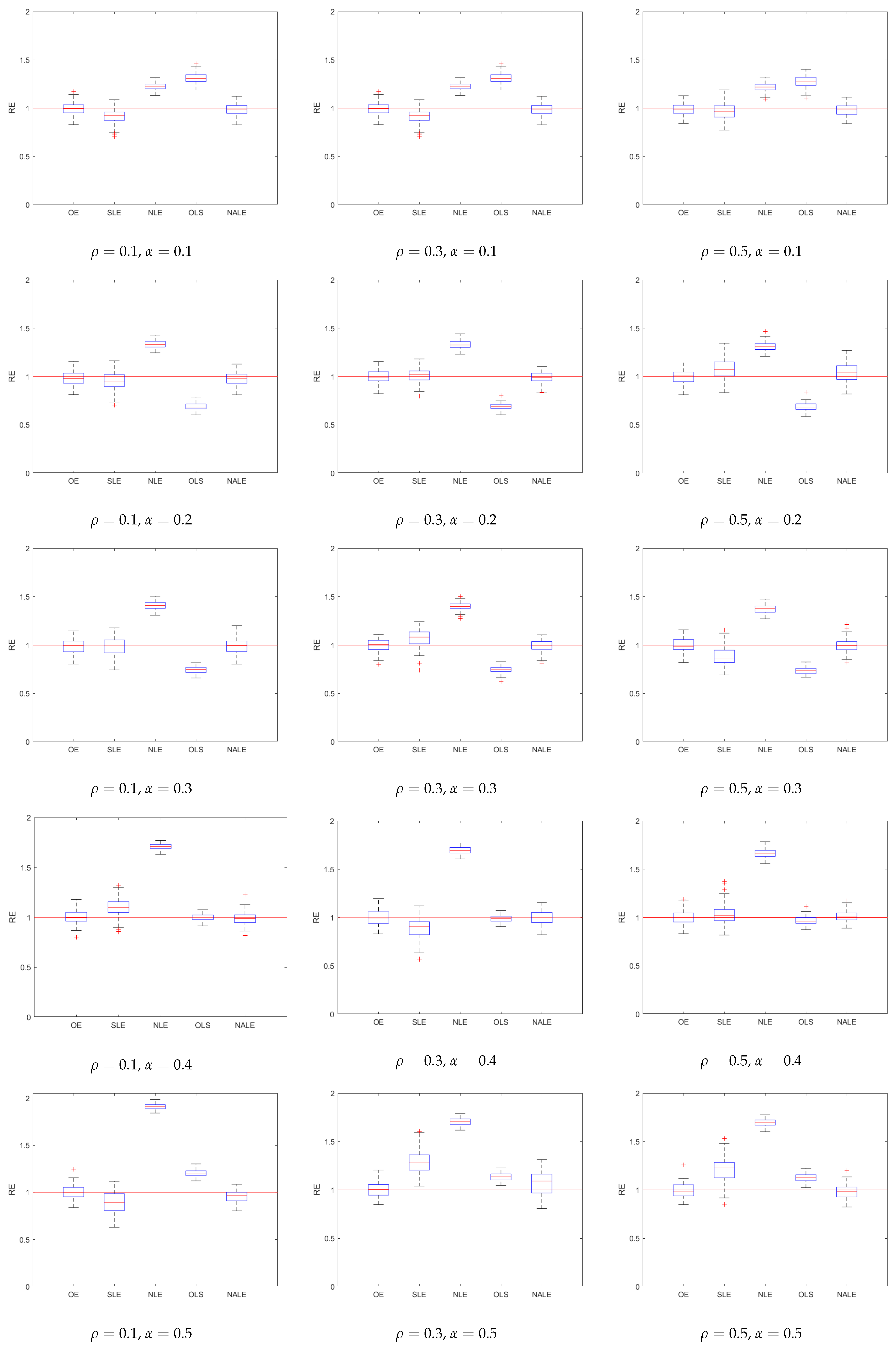
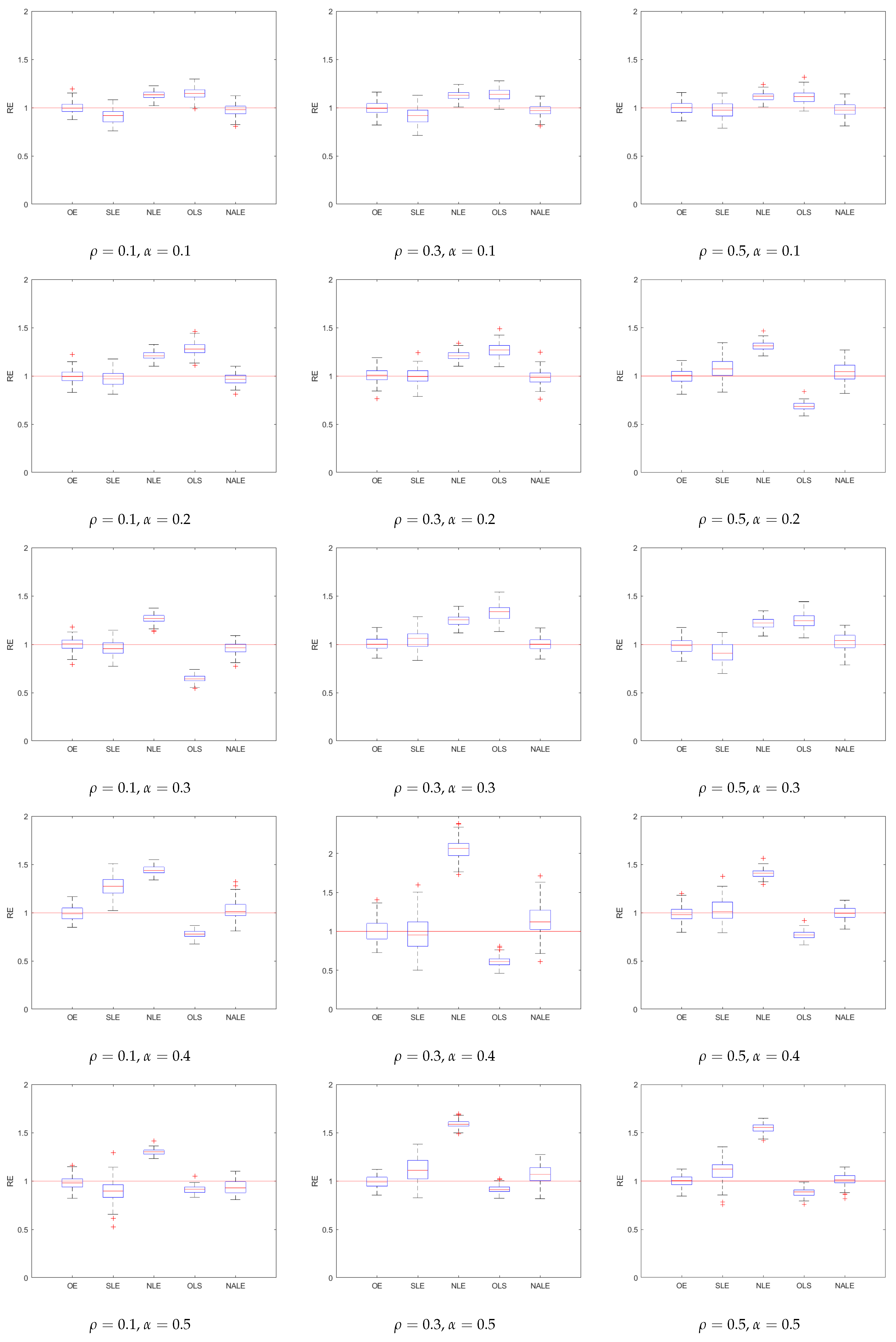
We, further, summarize the performances of various methods using boxplots, in Figure 1 and Figure 2. As one can easily see, the NALE is accurate and stable in all cases, while the OLE is less accurate, although it is, still, fairly stable. Further, the NALE performs well in extremely sparse scenarios. Another interesting point is that the NALE inherits the variable selection and parameter estimation of the adaptive lasso. Although we focus on the variance estimation in this work, the method performs well in estimating the regression coefficients as well.

Figure 1. Boxplots of 100 RE values for five estimators, true ${\sigma }^2=0.5$.

Figure 2. Boxplots of 100 RE values for five estimators, true ${\sigma }^2=1$.

6. Conclusions and Discussion

We proposed a novel approach for variance estimation that combines the reparameterized log-likelihood function and adaptive-lasso penalization. We have established the asymptotic properties of the NALE. The theory in this paper shows that the NALE converges at a faster rate than some other existing estimators, including the NLE, OLE and SLE. In addition, the NAL is closely related to the adaptive lasso, which makes its numerical calculation straightforward. We have used the PGA to obtain the NALE in numerical simulations. Our simulation results show that the NALE performs well and favorably against other existing methods, in most finite sample situations, especially in extremely sparse scenarios. However, the quality of the NALE depends on that of the initial estimator used in its numerical optimization, and the poor performance of the initial estimator may result in the poor performance of the NALE.

7. Regularity Conditions and Proofs

This section provides theoretical proofs. We first state the following regularity conditions.

Condition 1.

With probability approaching one, the initial estimator satisfies $\parallel {\tilde{\mathit{\beta }}}^{\mathrm{ini}}-{\mathit{\beta }}^{*}{\parallel }_2\le C_2\sqrt{s(logp)/n}$.

Condition 2.

$p_{\lambda }^{\prime }(t)$ is non-increasing in $t\in (0,\infty )$ and is Lipschitz with constant $C_3$, that is,

$$|p_{{\lambda }_n}^{\prime }(|t_1|)-p_{{\lambda }_n}^{\prime }(|t_2|)|\le C_3|t_1-t_2|$$

for any $t_1$, $t_2\in \mathbb{R}$. Moreover, $p_{{\lambda }_n}^{\prime }(C_2\sqrt{slogp/n})>(1/2)p_{{\lambda }_n}^{\prime }(0+)$ for sufficiently large n, where $C_2$ is defined in Condition 1.

Condition 3.

There exist positive constants $0<c_{\min }<c_{\max }<\infty$, such that

$$c_{\min }\le {\lambda }_{\min }\left(\frac{1}{n}{\mathit{X}}_{{\mathcal{A}}_0}^T{\mathit{X}}_{{\mathcal{A}}_0}\right)\le {\lambda }_{\max }\left(\frac{1}{n}{\mathit{X}}_{{\mathcal{A}}_0}^T{\mathit{X}}_{{\mathcal{A}}_0}\right)\le c_{\max },$$

and

$${\parallel \frac{1}{n}{\mathit{X}}_{{\mathcal{A}}_0^c}^T{\mathit{X}}_{{\mathcal{A}}_0}\parallel }_{2,\infty }<\frac{{\lambda }_n}{4\parallel {\mathit{w}}_{{\mathcal{A}}_0^c}^{-1}{\parallel }_{\infty }{a}_n},$$

where ${\parallel \mathit{B}\parallel }_{2,\infty }={max}_{{\parallel \mathit{v}\parallel }_2\le 1}{\parallel \mathit{B}\mathit{v}\parallel }_{\infty }$, ${\mathit{w}}_{{\mathcal{A}}_0^c}^{-1}={(w_{s+1}^{-1},\dots ,w_p^{-1})}^T$, $a_n$ is defined in Theorem 1.

Condition 4.

The true coefficients satisfy ${min}_{i\in {\mathcal{A}}_0}|{\mathit{\beta }}_i^{*}|\gg \sqrt{(s(2logp+2L))/n}$. Moreover, it holds $p_{{\lambda }_n}^{″}(t)=o(s^{-1}{\lambda }_n^{-1}{(2logp+2L)}^{-1/2})$ for any $t>{min}_{i\in {\mathcal{A}}_0}|{\mathit{\beta }}_i^{*}|/2$ and $L>0$.

As we pointed out in Remark 1, the lasso estimator ${\mathit{\beta }}_{\mathrm{lasso}}$ satisfies Condition 1. Condition 2 affects the bound between ${\widehat{\mathit{\beta }}}_{{\lambda }_n}$ and ${\mathit{\beta }}^{*}$ and is used in the proof of Theorem 1. Further, it determines the bound between ${\widehat{\sigma }}_{{\lambda }_n}^2$ and ${\sigma }_{\mathrm{oracle}}^2$. The first part of Condition 3 is a very common regularity condition (see [4,12,23]) in high-dimensional regression. The remaining part is similar to Condition 3 in [23], which is used in the proofs of Theorems 1 and 2. Condition 4 is needed in the analysis of Corollary 1.

Proof of Proposition 1.

(i)

Since $({\widehat{\mathit{\theta }}}_{{\lambda }_n},{\widehat{\varphi }}_{{\lambda }_n})$ is a solution of (2), ${\widehat{\mathit{\theta }}}_{{\lambda }_n}$ is a solution of the problem

$$\underset{{\mathit{\theta }}_{{\lambda }_n}\in {\mathbb{R}}^p}{min}L(\mathit{\theta },{\widehat{\varphi }}_{{\lambda }_n})+{\lambda }_n{\parallel \mathit{w}\circ \mathit{\theta }\parallel }_1.$$

Hence, by optimality of the above problem, we have

$$-{\mathit{X}}^T\mathit{y}+{\mathit{X}}^T\mathit{X}\frac{{\widehat{\mathit{\theta }}}_{{\lambda }_n}}{{\widehat{\varphi }}_{{\lambda }_n}}+n{\lambda }_n\mathit{w}\circ \widehat{\mathit{g}}=0,$$

where $\widehat{\mathit{g}}\in \partial (\parallel {\widehat{\mathit{\theta }}}_{{\lambda }_n}{\parallel }_1)$. It follows that

$$-{\mathit{X}}^T\mathit{y}+{\mathit{X}}^T\mathit{X}{\widehat{\mathit{\beta }}}_{{\lambda }_n}+n{\lambda }_n\mathit{w}\circ \widehat{\mathit{g}}=0.$$

Since $\mathrm{sign}({\widehat{\mathit{\theta }}}_{{\lambda }_n})=\mathrm{sign}({\widehat{\mathit{\beta }}}_{{\lambda }_n})$, we have $\partial (\parallel {\widehat{\mathit{\theta }}}_{{\lambda }_n}{\parallel }_1)=\partial (\parallel {\widehat{\mathit{\beta }}}_{{\lambda }_n}{\parallel }_1)$, which, further, implies that ${\widehat{\mathit{\beta }}}_{{\lambda }_n}$ is a solution of the adaptive lasso (4).

(ii)

Since $({\widehat{\mathit{\theta }}}_{{\lambda }_n},{\widehat{\varphi }}_{{\lambda }_n})$ is a solution of (2), by optimality of problem (2), we have

$$-{\mathit{X}}^T\mathit{y}+{\mathit{X}}^T\mathit{X}\frac{{\widehat{\mathit{\theta }}}_{{\lambda }_n}}{{\widehat{\varphi }}_{{\lambda }_n}}+n\lambda \mathit{w}\circ \widehat{\mathit{g}}=0,-\frac{1}{{\widehat{\varphi }}_{{\lambda }_n}}+\frac{1}{n}{\parallel \mathit{y}\parallel }_2^2-\frac{\parallel \mathit{X}{\widehat{\mathit{\theta }}}_{{\lambda }_n}{\parallel }_2^2}{n{\widehat{\varphi }}_{{\lambda }_n}^2}=0,$$

where $\widehat{\mathit{g}}\in \partial (\parallel {\widehat{\mathit{\theta }}}_{{\lambda }_n}{\parallel }_1)$. Therefore, we have

$$\begin{array}{c}\hfill -{\mathit{X}}^T\mathit{y}+{\mathit{X}}^T\mathit{X}{\widehat{\mathit{\beta }}}_{{\lambda }_n}+n{\lambda }_n\mathit{w}\circ \widehat{\mathit{g}}=0,-\frac{1}{{\widehat{\varphi }}_{{\lambda }_n}}+\frac{1}{n}{\parallel \mathit{y}\parallel }_2^2-\frac{\parallel \mathit{X}{\widehat{\mathit{\theta }}}_{{\lambda }_n}{\parallel }_2^2}{n{\widehat{\varphi }}_{{\lambda }_n}^2}=0.\end{array}$$

(7)

Since $\partial (\parallel {\widehat{\mathit{\theta }}}_{{\lambda }_n}{\parallel }_1)=\partial (\parallel {\widehat{\mathit{\beta }}}_{{\lambda }_n}{\parallel }_1)$, we have $\widehat{\mathit{g}}\in \partial (\parallel {\widehat{\mathit{\beta }}}_{{\lambda }_n}{\parallel }_1)$. Further,

$$\begin{array}{c}\hfill {\widehat{\mathit{\beta }}}_{{\lambda }_n}^T(\mathit{w}\circ \widehat{\mathit{g}})=\sum _{i=1}^p{w}_i{\widehat{\beta }}_i{\widehat{g}}_i=\sum _{i=1}^p|w_i{\widehat{\beta }}_i|=\parallel \mathit{w}\circ \widehat{\mathit{\beta }}{\parallel }_1.\end{array}$$

(8)

Combining (7) and (8), we obtain

$$0=-{\widehat{\mathit{\beta }}}_{{\lambda }_n}^T{\mathit{X}}^T\mathit{y}+\parallel \mathit{X}{\widehat{\mathit{\beta }}}_{{\lambda }_n}{\parallel }_2^2+{\lambda }_n{\parallel \mathit{w}\circ {\widehat{\mathit{\beta }}}_{{\lambda }_n}\parallel }_1,{\widehat{\sigma }}_{{\lambda }_n}^2=\frac{1}{n}\left({\parallel \mathit{y}\parallel }_2^2-{\parallel \mathit{X}{\widehat{\mathit{\beta }}}_{{\lambda }_n}\parallel }_2^2\right).$$

Further, by the first term in (7),

$$\begin{array}{ccc}\hfill \parallel \mathit{y}-\mathit{X}{\widehat{\mathit{\beta }}}_{{\lambda }_n}{\parallel }_2^2& =& {\parallel \mathit{y}\parallel }_2^2-{\parallel \mathit{X}{\widehat{\mathit{\beta }}}_{{\lambda }_n}\parallel }_2^2+2\left(\parallel \mathit{X}{\widehat{\mathit{\beta }}}_{{\lambda }_n}{\parallel }_2^2-{\mathit{y}}^T\mathit{X}{\widehat{\mathit{\beta }}}_{{\lambda }_n}\right)\hfill \\ & =& {\parallel \mathit{y}\parallel }_2^2-\parallel \mathit{X}{\widehat{\mathit{\beta }}}_{{\lambda }_n}{\parallel }_2^2-2{\lambda }_n{\parallel \mathit{w}\circ \widehat{\mathit{\beta }}\parallel }_1.\hfill \end{array}$$

Combining the above equality and the second term in (7), we have

$${\widehat{\sigma }}_{{\lambda }_n}^2=\frac{1}{n}\left({\parallel \mathit{y}\parallel }_2^2-{\parallel \mathit{X}{\widehat{\mathit{\beta }}}_{{\lambda }_n}\parallel }_2^2\right)=\parallel \mathit{y}-\mathit{X}{\widehat{\mathit{\beta }}}_{{\lambda }_n}{\parallel }_2^2+2{\lambda }_n{\parallel \mathit{w}\circ {\widehat{\mathit{\beta }}}_{{\lambda }_n}\parallel }_1,$$

which implies that ${\widehat{\sigma }}_{{\lambda }_n}^2$ is the optimal value of the adaptive lasso (4).  □

Proof of Lemma 1.

From Proposition 1, we have

$$\begin{array}{c}\hfill {\widehat{\sigma }}_{{\lambda }_n}^2\le \frac{1}{n}\parallel \mathit{y}-\mathit{X}{\mathit{\beta }}^{*}{\parallel }_2^2+2{\lambda }_n\parallel \mathit{w}\circ {\mathit{\beta }}^{*}{\parallel }_1=\frac{1}{n}{\parallel \mathit{\epsilon }\parallel }_2^2+2{\lambda }_n{\parallel \mathit{w}\circ {\mathit{\beta }}^{*}\parallel }_1.\end{array}$$

(9)

Since the loss function in the adaptive lasso is convex, we have

$$\begin{array}{ccc}\hfill {\widehat{\sigma }}_{{\lambda }_n}^2& =& \frac{1}{n}\parallel \mathit{y}-\mathit{X}{\widehat{\mathit{\beta }}}_{{\lambda }_n}{\parallel }_2^2+2{\lambda }_n{\parallel \mathit{w}\circ {\widehat{\mathit{\beta }}}_{{\lambda }_n}\parallel }_1\hfill \\ & \ge & \frac{1}{n}{\parallel \mathit{y}-\mathit{X}{\mathit{\beta }}^{*}\parallel }_2^2+{[\frac{2}{n}{\mathit{X}}^T({\mathit{X}}^T{\mathit{\beta }}^{*}-\mathit{y})]}^T({\widehat{\mathit{\beta }}}_{{\lambda }_n}-{\mathit{\beta }}^{*})\hfill \\ & =& \frac{1}{n}{\parallel \mathit{\epsilon }\parallel }_2^2-\frac{2}{n}{\mathit{\epsilon }}^T\mathit{X}({\widehat{\mathit{\beta }}}_{{\lambda }_n}-{\mathit{\beta }}^{*})\hfill \\ & \ge & \frac{1}{n}{\parallel \mathit{\epsilon }\parallel }_2^2-2\parallel \frac{1}{n}{\mathit{\epsilon }}^T{\mathit{X}\parallel }_{\infty }{\parallel {\widehat{\mathit{\beta }}}_{{\lambda }_n}-{\mathit{\beta }}^{*}\parallel }_1\hfill \\ & \ge & \frac{1}{n}{\parallel \mathit{\epsilon }\parallel }_2^2-2{\lambda }_n{\parallel {\widehat{\mathit{\beta }}}_{{\lambda }_n}-{\mathit{\beta }}^{*}\parallel }_1.\hfill \end{array}$$

(10)

Combining inequalities (9) and (10), we obtain

$$|{\widehat{\sigma }}_{{\lambda }_n}^2-\frac{1}{n}{\parallel \mathit{\epsilon }\parallel }_2^2|\le max\{2{\lambda }_n\parallel \mathit{w}\circ {\mathit{\beta }}^{*}{\parallel }_1,2\parallel \frac{1}{n}{\mathit{\epsilon }}^T{\mathit{X}\parallel }_{\infty }\parallel {\widehat{\mathit{\beta }}}_{{\lambda }_n}-{\mathit{\beta }}^{*}{\parallel }_1\},$$

which completes the proof. □

Proof of Theorem 1.

Since problem (4) is a convex optimization, by Theorem 1 of [25], it suffices to show that, with probability tending to 1, there exists a minimizer ${\widehat{\mathit{\beta }}}_{{\lambda }_n}$ of problem (4) that satisfies

$$\begin{array}{c}{\mathit{X}}_{{\mathcal{A}}_0}^T(\mathit{y}-\mathit{X}{\widehat{\mathit{\beta }}}_{{\lambda }_n})-n{\lambda }_n{\mathit{w}}_{{\mathcal{A}}_0}\circ {\widehat{\mathit{g}}}_{{\mathcal{A}}_0}=\mathbf{0},\hfill \end{array}$$

(11)

$$\begin{array}{c}\parallel {\mathit{X}}_{{\mathcal{A}}_0^c}^T(\mathit{y}-\mathit{X}{\widehat{\mathit{\beta }}}_{{\lambda }_n}){\parallel }_{\infty }<n{\lambda }_n{\mathit{w}}_{{\mathcal{A}}_0^c},\hfill \end{array}$$

(12)

$$\begin{array}{c}{\lambda }_{\min }\left(\frac{1}{n}{\mathit{X}}_{{\mathcal{A}}_0}^T{\mathit{X}}_{{\mathcal{A}}_0}\right)\ge c_{\min }.\hfill \end{array}$$

(13)

where $\widehat{\mathit{g}}\in \partial {\parallel \widehat{\mathit{\beta }}\parallel }_1$.

Let ${\mathit{\xi }}_1={\mathit{X}}_{{\mathcal{A}}_0}^T\mathit{\epsilon }$ and ${\mathit{\xi }}_2={\mathit{X}}_{{\mathcal{A}}_0^c}^T\mathit{\epsilon }$. Since $\parallel {\mathit{X}}_j{\parallel }_2^2=n$ and $\mathit{\epsilon }\sim N(0,{\sigma }^2{I}_n)$, it follows from Corollary 4.3 in [26] that, for any $L>0$,

$$\begin{array}{c}\hfill P\left\{\frac{\parallel {\mathit{X}}^T{\mathit{\epsilon }\parallel }_{\infty }}{n\sigma }>\sqrt{\frac{2logp+2L}{n}}\right\}\le e^{-L}.\end{array}$$

(14)

Now we show that there exists a minimizer $\widehat{\mathit{\beta }}$ of problem (4) satisfies conditions (11)–(13).

Equation (11): Consider the minimizer of problem (4) in the subspace $\{\mathit{\beta }={({\mathit{\beta }}_{{\mathcal{A}}_0}^T,{\mathit{\beta }}_{{\mathcal{A}}_0^c}^T)}^T:{\mathit{\beta }}_{{\mathcal{A}}_0^c}=\mathbf{0}\}$. Let $\mathit{\beta }={({\mathit{\beta }}_{{\mathcal{A}}_0}^T,{\mathbf{0}}^T)}^T$, where ${\mathit{\beta }}_{{\mathcal{A}}_0}={\mathit{\beta }}_{{\mathcal{A}}_0}^{*}+{\tilde{a}}_n{\mathit{v}}_{{\mathcal{A}}_0}\in {\mathbb{R}}^s$ with ${\tilde{a}}_n=\sqrt{s(2logp+2L)/n}+2{\lambda }_n(\parallel {\mathit{w}}_{{\mathcal{A}}_0}^{*}{\parallel }_2+C_2{C}_3\sqrt{s(logp)/n})$, $\parallel v_{{\mathcal{A}}_0}{\parallel }_2=C$, and $C>0$ is some large enough constant. Note that

$$\begin{array}{c}\hfill L_n({\mathit{\beta }}_{{\mathcal{A}}_0}^{*}+{\tilde{a}}_n{\mathit{v}}_{{\mathcal{A}}_0},\mathbf{0})-L_n({\mathit{\beta }}_{{\mathcal{A}}_0}^{*},\mathbf{0})=I_1({\mathit{v}}_{{\mathcal{A}}_0})+I_2({\mathit{v}}_{{\mathcal{A}}_0}),\end{array}$$

(15)

where $I_1({\mathit{v}}_{{\mathcal{A}}_0})=\frac{1}{n}\parallel \mathit{X}({\mathit{\beta }}^{*}+{\tilde{a}}_n\mathit{v}){-\mathit{y}\parallel }_2^2-\frac{1}{n}{\parallel \mathit{X}{\mathit{\beta }}^{*}-\mathit{y}\parallel }_2^2$, $I_2({\mathit{v}}_{{\mathcal{A}}_0})=2{\lambda }_n\parallel {\mathit{w}}_{{\mathcal{A}}_0}\circ ({\mathit{\beta }}_{{\mathcal{A}}_0}^{*}+{\tilde{a}}_n{\mathit{v}}_{{\mathcal{A}}_0}){\parallel }_1-2{\lambda }_n{\parallel {\mathit{w}}_{{\mathcal{A}}_0}\circ {\mathit{\beta }}_{{\mathcal{A}}_0}^{*}\parallel }_1$. For $I_1({\mathit{v}}_{{\mathcal{A}}_0})$, by (14), we have

$$\begin{array}{ccc}\hfill I_1({\mathit{v}}_{{\mathcal{A}}_0})& =& \frac{1}{n}\parallel \mathit{X}({\mathit{\beta }}^{*}+{\tilde{a}}_n\mathit{v}){-\mathit{y}\parallel }_2^2-\frac{1}{n}{\parallel \mathit{X}{\mathit{\beta }}^{*}-\mathit{y}\parallel }_2^2\hfill \\ & =& \frac{1}{n}{\tilde{\mathit{a}}}_n^2{\mathit{v}}^T{\mathit{X}}^T\mathit{X}\mathit{v}+\frac{2}{n}{\mathit{\epsilon }}^T\mathit{X}{\tilde{\mathit{a}}}_n\mathit{v}\hfill \\ & =& \frac{1}{n}{\tilde{\mathit{a}}}_n^2{\mathit{v}}_{{\mathcal{A}}_0}^T{\mathit{X}}_{{\mathcal{A}}_0}^T{\mathit{X}}_{{\mathcal{A}}_0}{\mathit{v}}_{{\mathcal{A}}_0}+\frac{2}{n}{\tilde{\mathit{a}}}_n{\mathit{\epsilon }}^T{\mathit{X}}_{{\mathcal{A}}_0}{\mathit{v}}_{{\mathcal{A}}_0}\hfill \\ & \ge & c_{\min }{\tilde{\mathit{a}}}_n^2\parallel {\mathit{v}}_{{\mathcal{A}}_0}{\parallel }_2^2-2{\tilde{\mathit{a}}}_n\parallel \frac{{\mathit{\xi }}_1}{n}{\parallel }_2{\parallel {\mathit{v}}_{{\mathcal{A}}_0}\parallel }_2\hfill \\ & \ge & c_{\min }{\tilde{\mathit{a}}}_n^2\parallel {\mathit{v}}_{{\mathcal{A}}_0}{\parallel }_2^2-2\sigma {\tilde{\mathit{a}}}_n\sqrt{s(2logp+2L)/n}{\parallel {\mathit{v}}_{{\mathcal{A}}_0}\parallel }_2,\hfill \end{array}$$

(16)

where the last inequality holds, due to ${\parallel ·\parallel }_2\le \sqrt{s}{\parallel ·\parallel }_{\infty }$. For $I_2({\mathit{v}}_{{\mathcal{A}}_0})$, we have

$$\begin{array}{ccc}\hfill I_2({\mathit{v}}_{{\mathcal{A}}_0})& =& 2{\lambda }_n\parallel {\mathit{w}}_{{\mathcal{A}}_0}\circ ({\mathit{\beta }}_{{\mathcal{A}}_0}^{*}+{\tilde{a}}_n{\mathit{v}}_{{\mathcal{A}}_0}){\parallel }_1-2{\lambda }_n{\parallel {\mathit{w}}_{{\mathcal{A}}_0}\circ {\mathit{\beta }}_{{\mathcal{A}}_0}^{*}\parallel }_1\hfill \\ & \le & 2{\lambda }_n\parallel {\mathit{w}}_{{\mathcal{A}}_0}\circ ({\tilde{a}}_n{\mathit{v}}_{{\mathcal{A}}_0}){\parallel }_1\le 2{\tilde{a}}_n{\lambda }_n\parallel {\mathit{w}}_{{\mathcal{A}}_0}{\parallel }_2{\parallel {\mathit{v}}_{{\mathcal{A}}_0}\parallel }_2.\hfill \end{array}$$

(17)

By the two-steps procedure of weight vector and Condition 2, it holds that

$$\begin{array}{ccc}\hfill \parallel {\mathit{w}}_{{\mathcal{A}}_0}{\parallel }_2& \le & \parallel {\mathit{w}}_{{\mathcal{A}}_0}-{\mathit{w}}_{{\mathcal{A}}_0}^{*}{\parallel }_2+\parallel {\mathit{w}}_{{\mathcal{A}}_0}^{*}{\parallel }_2\le C_3\parallel {\tilde{\mathit{\beta }}}_{{\mathcal{A}}_0}^{\mathrm{ini}}-{\mathit{\beta }}_{{\mathcal{A}}_0}^{*}{\parallel }_2+{\parallel {\mathit{w}}_{{\mathcal{A}}_0}^{*}\parallel }_2\hfill \\ & \le & C_2{C}_3\sqrt{s(logp)/n}+{\parallel {\mathit{w}}_{{\mathcal{A}}_0}^{*}\parallel }_2.\hfill \end{array}$$

(18)

Hence, combining (15)–(18) yields

$$\begin{array}{ccc}\hfill L_n({\mathit{\beta }}_{{\mathcal{A}}_0}^{*}+{\tilde{a}}_n{\mathit{v}}_{{\mathcal{A}}_0},\mathbf{0})-L_n({\mathit{\beta }}_{{\mathcal{A}}_0}^{*},\mathbf{0})& \ge & c_{\min }{\tilde{a}}_n^2\parallel {\mathit{v}}_{{\mathcal{A}}_0}{\parallel }_2^2-2\sigma {\tilde{a}}_n\sqrt{s(2logp+2L)/n}{\parallel {\mathit{v}}_{{\mathcal{A}}_0}\parallel }_2\hfill \\ & & -2{\tilde{a}}_n{\lambda }_n(C_2{C}_3\sqrt{s(logp)/n}+\parallel {\mathit{w}}_{{\mathcal{A}}_0}^{*}{\parallel }_2)\parallel {\mathit{v}}_{{\mathcal{A}}_0}{\parallel }_2.\hfill \end{array}$$

Taking a large enough C, we have obtained, with probability tending to one,

$$L_n({\mathit{\beta }}_{{\mathcal{A}}_0}^{*}+{\tilde{a}}_n{\mathit{v}}_{{\mathcal{A}}_0},\mathbf{0})-L_n({\mathit{\beta }}_{{\mathcal{A}}_0}^{*},\mathbf{0})>0.$$

It follows, immediately, that, with probability approaching one, there exists a minimizer ${\widehat{\mathit{\beta }}}_{{\mathcal{A}}_0}$ of problem (4), subject to subspace $\{\mathit{\beta }={({\mathit{\beta }}_{{\mathcal{A}}_0}^T,{\mathit{\beta }}_{{\mathcal{A}}_0^c}^T)}^T:{\mathit{\beta }}_{{\mathcal{A}}_0^c}=\mathbf{0}\}$, such that $\parallel {\widehat{\mathit{\beta }}}_{{\mathcal{A}}_0}-{\mathit{\beta }}_{{\mathcal{A}}_0}^{*}{\parallel }_2\le C_4{\tilde{a}}_n\equiv a_n$, with some constant $C_4>0$. Therefore, equality (11) holds, by the optimality theory.

Inequality (12): It remains to be proven that with asymptotic probability 1, (12) holds. Then, by optimality theory, ${\widehat{\mathit{\beta }}}_{{\lambda }_n}={({\widehat{\mathit{\beta }}}_{{\mathcal{A}}_0}^T,{\mathbf{0}}^T)}^T$ is the unique global minimizer of problem (4).

By triangle inequality, we have

$$\begin{array}{c}\hfill \parallel {\mathit{X}}_{{\mathcal{A}}_0^c}^T(\mathit{y}-\mathit{X}\widehat{\mathit{\beta }}){\parallel }_{\infty }\le \parallel {\mathit{X}}_{{\mathcal{A}}_0^c}^T(\mathit{y}-\mathit{X}{\mathit{\beta }}^{*}){\parallel }_{\infty }+{\parallel {\mathit{X}}_{{\mathcal{A}}_0^c}^T\mathit{X}({\mathit{\beta }}^{*}-\widehat{\mathit{\beta }})\parallel }_{\infty }.\end{array}$$

(19)

Further, by Condition 1, we have $|{\tilde{\mathit{\beta }}}_i^{\mathrm{ini}}|\le C_2\sqrt{s(logp)/n}$ with probability approaching one, where $i\in {\mathcal{A}}_0^c$. Moreover, by the definition of the fold-concave penalty function,

$$\begin{array}{c}\hfill p_{{\lambda }_n}^{\prime }(|{\tilde{\mathit{\beta }}}_i^{\mathrm{ini}}|)\ge p_{{\lambda }_n}^{\prime }(C_2\sqrt{s(logp)/n}).\end{array}$$

(20)

Therefore, by Condition 2 and inequality (20), we conclude that

$$\begin{array}{c}\hfill \parallel {\mathit{w}}_{{\mathcal{A}}_0^c}^{-1}{\parallel }_{\infty }=\underset{i\in {\mathcal{A}}_0^c}{min}{p}_{{\lambda }_n}^{\prime }(|{\tilde{\mathit{\beta }}}_i^{\mathrm{ini}}{|)}^{-1}<\frac{2}{p_{{\lambda }_n}^{\prime }(0+)}=2{\parallel {({\mathit{w}}_{{\mathcal{A}}_0^c}^{*})}^{-1}\parallel }_{\infty }.\end{array}$$

(21)

Thus, for the first term of the right hand of inequality (19), by (14) and the condition that ${min}_{i\in {\mathcal{A}}_0^c}\{w_i^{*}\}>C_1^{-1}$, with probability approaching one,

$$\begin{array}{ccc}\hfill \frac{1}{n}{\parallel {\mathit{X}}_{{\mathcal{A}}_0^c}^T(\mathit{y}-\mathit{X}{\mathit{\beta }}^{*})\parallel }_{\infty }& =& \frac{1}{n}{\parallel {\mathit{X}}_{{\mathcal{A}}_0^c}^T\mathit{\epsilon }\parallel }_{\infty }\hfill \\ & <& \sigma \sqrt{\frac{2logp+2L}{n}}=\frac{{\lambda }_n}{4C_1}<\frac{{\lambda }_n}{4\parallel {({\mathit{w}}_{{\mathcal{A}}_0^c}^{*})}^{-1}{\parallel }_{\infty }}<\frac{{\lambda }_n}{2\parallel {\mathit{w}}_{{\mathcal{A}}_0^c}^{-1}{\parallel }_{\infty }}.\hfill \end{array}$$

(22)

As for the second term of right hand of inequality (19), by Condition 3, inequality (21) and inequality (14), with probability approaching one, we have

$$\begin{array}{ccc}\hfill \frac{1}{n}{\parallel {\mathit{X}}_{{\mathcal{A}}_0^c}^T\mathit{X}({\mathit{\beta }}^{*}-\widehat{\mathit{\beta }})\parallel }_{\infty }& \le & \frac{1}{n}\parallel {\mathit{X}}_{{\mathcal{A}}_0^c}^T{\mathit{X}}_{{\mathcal{A}}_0}{\parallel }_{2,\infty }{\parallel {\mathit{\beta }}_{{\mathcal{A}}_0}^{*}-{\widehat{\mathit{\beta }}}_{{\mathcal{A}}_0}\parallel }_2\hfill \\ & \le & \frac{{\lambda }_n}{4\parallel {({\mathit{w}}_{{\mathcal{A}}_0^c}^{*})}^{-1}{\parallel }_{\infty }}<\frac{{\lambda }_n}{2\parallel {\mathit{w}}_{{\mathcal{A}}_0^c}^{-1}{\parallel }_{\infty }}.\hfill \end{array}$$

(23)

Combining (19), (22) and (23), we obtain inequality (12).

Inequality (13): it follows from Condition 3 that with an asymptotic probability of one, inequality (13) holds. This completes the proof of Theorem 1. □

Proof of Theorem 2.

By equality (11), $(1/n){\mathit{X}}_{{\mathcal{A}}_0}^T(\mathit{y}-\mathit{X}{\widehat{\mathit{\beta }}}_{{\lambda }_n})-{\lambda }_n{\mathit{w}}_{{\mathcal{A}}_0}\circ {\widehat{\mathit{g}}}_{{\mathcal{A}}_0}=\mathbf{0}.$ Since $\mathit{y}-\mathit{X}{\mathit{\beta }}^{*}=\mathit{\epsilon }$, we have

$$\frac{1}{n}{\mathit{X}}_{{\mathcal{A}}_0}^T{\mathit{X}}_{{\mathcal{A}}_0}({\widehat{\mathit{\beta }}}_{{\mathcal{A}}_0}-{\mathit{\beta }}_{{\mathcal{A}}_0}^{*})=-{\lambda }_n{\mathit{w}}_{{\mathcal{A}}_0}\circ {\widehat{\mathit{g}}}_{{\mathcal{A}}_0}+\frac{1}{n}{\mathit{X}}_{{\mathcal{A}}_0}^T\mathit{\epsilon }.$$

Therefore,

$$\begin{array}{c}\hfill n^{1/2}{\mathit{\alpha }}_n^T({\widehat{\mathit{\beta }}}_{{\mathcal{A}}_0}-{\mathit{\beta }}_{{\mathcal{A}}_0}^{*})+n^{3/2}{\lambda }_n{\mathit{\alpha }}_n^T{({\mathit{X}}_{{\mathcal{A}}_0}^T{\mathit{X}}_{{\mathcal{A}}_0})}^{-1}{\mathit{w}}_{{\mathcal{A}}_0}\circ {\widehat{\mathit{g}}}_{{\mathcal{A}}_0}=n^{1/2}{\mathit{\alpha }}_n^T{({\mathit{X}}_{{\mathcal{A}}_0}^T{\mathit{X}}_{{\mathcal{A}}_0})}^{-1}{\mathit{X}}_{{\mathcal{A}}_0}^T\mathit{\epsilon }.\end{array}$$

(24)

By the first part of Condition 4 and the bound of ${\widehat{\mathit{\beta }}}_{{\lambda }_n}$ in Theoroem 1, we have $\mathrm{sign}({\widehat{\mathit{\beta }}}_{{\mathcal{A}}_0})=\mathrm{sign}({\mathit{\beta }}_{{\mathcal{A}}_0}^{*})$. Then, ${\widehat{\mathit{g}}}_{{\mathcal{A}}_0}={\mathit{g}}_{{\mathcal{A}}_0}^{*}$. In addition, by the second part in condition 4,

$$\begin{array}{c}\hfill {\mathit{w}}_{{\mathcal{A}}_0}={\mathit{w}}_{{\mathcal{A}}_0}^{*}+\mathit{\zeta }({\widehat{\mathit{\beta }}}_{{\mathcal{A}}_0}-{\mathit{\beta }}_{{\mathcal{A}}_0}^{*}),\end{array}$$

where $\mathit{\zeta }=\mathrm{diag}{(p_{{\lambda }_n}^{″}({\tilde{\beta }}_1),\dots ,p_{{\lambda }_n}^{″}({\tilde{\beta }}_s))}^T\in {\mathbb{R}}^{s\times s}$ and $\tilde{\mathit{\beta }}\in {\mathbb{R}}^s$ lie on the line segment $[{\widehat{\mathit{\beta }}}_{{\mathcal{A}}_0},{\mathit{\beta }}_{{\mathcal{A}}_0}^{*}]$. It follows that $\parallel \mathit{\zeta }({\widehat{\mathit{\beta }}}_{{\mathcal{A}}_0}-{\mathit{\beta }}_{{\mathcal{A}}_0}^{*})\circ {\mathit{g}}_{{\mathcal{A}}_0}^{*}{\parallel }_2={\parallel \mathit{\zeta }({\widehat{\mathit{\beta }}}_{{\mathcal{A}}_0}-{\mathit{\beta }}_{{\mathcal{A}}_0}^{*})\parallel }_2=o({\lambda }_n^{-1}\sqrt{1/n})$. Further, since

$$\begin{array}{c}\hfill |n^{3/2}{\lambda }_n{\mathit{\alpha }}_n^T{({\mathit{X}}_{{\mathcal{A}}_0}^T{\mathit{X}}_{{\mathcal{A}}_0})}^{-1}[\mathit{\zeta }({\widehat{\mathit{\beta }}}_{{\mathcal{A}}_0}-{\mathit{\beta }}_{{\mathcal{A}}_0}^{*})\circ {\mathit{g}}_{{\mathcal{A}}_0}^{*}]|\le n^{1/2}{\lambda }_n{c}_{\max }\parallel {\mathit{\alpha }}_n{\parallel }_2{\parallel \mathit{\zeta }({\widehat{\mathit{\beta }}}_{{\mathcal{A}}_0}-{\mathit{\beta }}_{{\mathcal{A}}_0}^{*})\parallel }_2=o(1),\end{array}$$

we have, for the second term of the left hand of (24),

$$\begin{array}{c}\hfill n^{3/2}{\lambda }_n{\mathit{\alpha }}_n^T{({\mathit{X}}_{{\mathcal{A}}_0}^T{\mathit{X}}_{{\mathcal{A}}_0})}^{-1}{\mathit{w}}_{{\mathcal{A}}_0}\circ {\widehat{\mathit{g}}}_{{\mathcal{A}}_0}=n^{3/2}{\lambda }_n{\mathit{\alpha }}_n^T{({\mathit{X}}_{{\mathcal{A}}_0}^T{\mathit{X}}_{{\mathcal{A}}_0})}^{-1}{\mathit{w}}_{{\mathcal{A}}_0}\circ {\mathit{g}}_{{\mathcal{A}}_0}^{*}+o(1).\end{array}$$

Finally, the result follows, by verifying the conditions of the Lindeberg–Feller central limit theorem, in the same way as in the proof of Theorem 2 in [4]. □

Proof of Theorem 4.

For any $M>1$, take $L=(M-1)logp$ and denote $Z_n=({\widehat{\sigma }}_{{\lambda }_n}^2-\frac{1}{n}{\parallel \mathit{\epsilon }\parallel }_2^2{)}^2$. Then, by Theorems 1 and 3, we have

$$P(Z_n>M{b}_n^2)\le e^{-(M-1)logp}.$$

It follows that

$$\begin{array}{ccc}\hfill E\left(\frac{Z_n}{b_n^2}\right)& =& {\int }_0^{\infty }P\left(\frac{Z_n}{b_n^2}>t\right)dt={\int }_0^{M}P\left(\frac{Z_n}{b_n^2}>t\right)dt+{\int }_M^{\infty }P\left(\frac{Z_n}{b_n^2}>t\right)dt\hfill \\ & \le & M+{\int }_M^{\infty }{e}^{-(M-1)logp}dt=M+\frac{p^{1-M}}{logp}.\hfill \end{array}$$

(25)

Further, since ${\sigma }^{-2}{\parallel \mathit{\epsilon }\parallel }_2^2\sim {\chi }^2(n)$, we have

$$E\left(\frac{1}{n}{\parallel \mathit{\epsilon }\parallel }_2^2\right)={\sigma }^2,\mathrm{Var}\left(\frac{1}{n}{\parallel \mathit{\epsilon }\parallel }_2^2\right)=\frac{2{\sigma }^4}{n}.$$

By the proof of Theorem 12 in [13], we have

$$\begin{array}{c}\hfill E\left\{{({\widehat{\sigma }}_{{\lambda }_n}^2-{\sigma }^2)}^2\right\}\le {\left\{{\left[E\left\{{\left({\widehat{\sigma }}_{{\lambda }_n}^2-\frac{1}{n}{\parallel \mathit{\epsilon }\parallel }_2^2\right)}^2\right\}\right]}^{\frac{1}{2}}+{\left\{\mathrm{Var}(\frac{1}{n}\parallel \mathit{\epsilon }{\parallel }_2^2)\right\}}^{\frac{1}{2}}\right\}}^2.\end{array}$$

(26)

Combining (25) and (26), we obtain

$$\begin{array}{c}\hfill E\left\{{({\widehat{\sigma }}_{{\lambda }_n}^2-{\sigma }^2)}^2\right\}\le {\left[{\left(M+\frac{p^{1-M}}{logp}\right)}^{\frac{1}{2}}{b}_n^2+{\sigma }^2{\left(\frac{2}{n}\right)}^{\frac{1}{2}}\right]}^2.\end{array}$$

The proof is complete. □