Abstract
The current study focuses on the natural-convection flow of nanofluids with boundary layer over a circular cylinder of uniform thermal wall with varying magnetic force from 0 to 1.5, radiative effects from 0 to 1, heat generation effects from 0 to 1, and Joule heating effects from 0 to 1. The problem is represented in the form of partial differential equations. The dimensional form of the equations is converted into a dimensionless form with the help of suitable stream functions. Then, the resultant equations are further reduced into the system of first-ordered differential equations, and the Keller box scheme is applied to obtain a solution numerically with the help of MATLAB code. The numerical solutions for Nusselt number, skin friction coefficient, Sherwood number, velocity profile, temperature profile, and concentration profile are represented with the help of graphs. The most interesting fact of the analysis is the flow of the fluid; the heat-mass and energy transfer rates could be managed in a controlled way through slight variations in the Brownian motion parameter from 0.1 to 0.7, in the Lewis number from 1 to 40, in the Eckert number from 0.1 to 0.4, in the thermophoresis parameter from 0.1 to 0.7, in the Prandtl number from 0.1 to 0.7, and in the buoyancy ratio from 0.1 to 0.7, as it is here analyzed and discussed.
Keywords:
nanofluid; natural convective flow; horizontal circular cylinder; thermal radiation effect; Keller box scheme MSC:
76A02; 76F35; 76R10; 76M50
1. Introduction
The configuration of viscous and incompressible fluids flowing with natural convection over a cylinder of circular form lying parallel to the x-axis is important for many engineering processes. The applications of these types of processes are geophysical heat elimination, food storage and processing, metallurgy sciences, geothermal removal of nuclear and non-nuclear reactors, and various branches of engineering, such as mechanical, chemical, and civil engineering. The pioneering studies by Blasius et al. [1] discussed the boundary-layer flow over the horizontally placed circular form of a cylinder in 1908. They found the velocity profile and evaluated the momentum transport equation of the forced-convection boundary-layer flow. Since then, these studies have found a new space in the cabinet of many researchers. Later on, Markin et al. [2] were the first who examined the exact solution of a free-convection flow over the isothermal cylinder. Later on, they found the exact solution of the mixed convective flow over an isothermal cylinder with the wall of the cylinder having a fixed temperature with the help of the Gortler–Blasius series expansion along with the finite difference scheme [3]. With the help of Markin et al.’s work, Ingham and Pop [4] made a great contribution in this era. They determined the solution of a free convective flow over an isothermal horizontal cylinder numerically. Recently, Mohamed et al. [5] investigated the viscous-dissipation flow over a horizontal circular cylinder of a nanofluid with free-convection boundary layer.
Although water, oil, and ethylene mixtures are usually employed in many flows, the heat transfer rate is very poor in such fluids. Since thermal conductivity plays a vital role in the heat transfer from a surface to a fluid, for a better result, it is necessary to invent a fluid that gives a better result. For this purpose, nano-sized metallic particles have been added to fluids in recent years. The term “Nanofluid”, used for this kind of fluid, was first introduced by Choi and Eastman [6] in 1995. Nanofluids are a mixture of nano-sized particles such as oxides and carbides suspended in the base fluid. Nanofluids enable us to develop clean-energy-source devices such as smartphones and laptops. Some interesting and meaningful experiments and numerical research studies on nanofluids were conducted by [7,8,9,10,11]. They predicted some thermo-physical properties of nanofluids and showed the impact of these properties on the convective heat flow using different models. Eastman et al. [12] found that an increment of up to 40% in heat conductivity could be achieved using ethylene–glycol mixed with 0.3% volumetric copper nanoparticles of 10 nm in size. Das et al. [13] obtained an increment from 10% to 30% in thermal conduction with an aluminum–water mixture with 4% of alumina.
In radiation, waves are emitted or transferred in the form of energy from surface particles or through space. So, radiation also impacts the rate of thermal diffusion and other thermo-physical properties of a fluid. Therefore, the thermal radiation effects on various geometrical surfaces were considered by different researchers. Hossain and Alim [14] examined the impact of free convective heat transfer with radiation on a flow over a thin, vertically placed cylinder. Hossain et al. [15] extended this idea to mixed convective thermal transport over a cylinder with circular diameter. The mystery of viscous fluids being temperature-dependent on a cylinder with circular diameter having fixed wall temperature was revealed by him. A few years ago, Elbashbeshy et al. [16] found out the effects of the radiative transfer of a fluid with a heat source and sink on the natural-convection flow over a truncated cone. A letter by Zeeshan et al. [17] briefly explains the effect of radiative MHD and of diminishing the internal energy of flows on titanium dioxide nanofluid water.
The internal generation of heat in a fluid is an important factor for consideration. Some beneficial work has been presented by many researchers on free-convection flows over the horizontal circular form of a cylinder having heat generation effects. Heat-generating phenomena have a significant impact on the problem involving internal chemical reactions in a fluid. The impact of heat generation on a fluid alters the temperature distribution. Vajravelu and Hadjinolaou [18] determined the characteristics of heat generation of a viscous-fluid flow over a linear stretching surface. They considered heat generation in terms of the volumetric rate. Molla et al. [19] examined the influence of heat generation along with the natural convective flow over the isothermal horizontally placed circular form of a cylinder. After that, their work was further extended by Molla et al. [20], whose extension was a uniform heat flux. Meanwhile, their study was verified by Cheng [21] and further extended to a surface with a free convective boundary-layer flow over the horizontal and elliptical form of a cylinder with heat-generating effects and constant heat flux of the surface. Recently, Mohammed et al. [22] briefly studied the effects of viscous dissipation over a horizontal cylinder with a natural convective flow.
The magnetic hydrodynamic (MHD) effects on different surfaces represent an important area of study due to the large range of applications. The free-convection flow with MHD effects over the surface of different shapes has been studied by some researchers, and important results have been found. Hossain et al. [23] examined the heat flow rate in the presence of an MHD natural-convection flow over an oscillating and heated vertical flat plate. They obtained a solution with natural frequencies using the finite implicit scheme known as the Keller box method. Wilks [24] integrated the MHD natural convective flow with the vertical semi-infinite plate. Meanwhile, Azim and chowdhury [25] investigated the MHD effects along with the Joule heating effect and the heat generation effect over a horizontal circular cylinder and produced well-known results. The very next year, Azim [26] extended the same idea and produced a result with MHD and viscous dissipation effects. Later, Ellahi et al. [27] studied free convective and MHD nanofluids as well as flows over a single wall as well as multiple walls made of carbonated nanotubes and produced remarkable results. Furthermore, Nazeer et al. [28] extended that idea to produce results with the help of numerical simulations of MHD effects on a forced convective flow over a porous triangular cavity.
The above-cited contributions were restricted to a limited number of parameters variations applied numerically on selected surfaces at one time. None of them identified the natural convective flow of nanofluids including the viscous dissipation, magnetohydrodynamic, radiative, Joule heating, and heat generation effects over a horizontal circular cylinder. The governing partial differential equations are here solved and discussed numerically using the Keller box method and are presented graphically. To the best of our knowledge, until now, the presented problem has not been published by others yet.
2. Fundamental Governing Equations
Consider a circular cylinder with a horizontal axis having radius a normal to the axis of that cylinder. The fluid flowing over the horizontal cylinder is assumed to be a nanofluid, and it is immersed in an incompressible and viscous fluid with ambient temperature . Furthermore, the cylinder is heated with constant temperature known as , and the flow is steady and two-dimensional laminar natural convective with uniform heat flux. As magnetic effect M is not constant, constant magnetic field B0 is also applied. The cylindrical surface is measured according to the orthogonal coordinate system of and , where is considered to be a starting point as a lower stagnation point in the counter-clock-wise direction with the angle of , and is the coordinate axis normal to the coordinate . The physical model of the problem is shown in Figure 1.
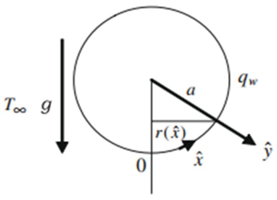
Figure 1.
Physical model of the problem.
Under the main assumptions of the law of conservation of mass, momentum and energy, the boundary-layer dimensional equations according to Boussinesq boundary-layer approximation are valid as shown below.
Continuity equation.
Momentum equation.
Energy equation.
where the following apply.
Concentration equation.
Assumptions for the Problem
The velocity components in the direction along and are and , respectively. Constant values such as and , and dynamic and kinematic viscosities have more important characteristic properties in the considered fluid. Moreover, g is the gravitational constant of the acceleration field acting on the fluid. The thermal expansion is , which controls the thermal behavior of the fluid, while is the coefficient of concentration expansion. As the fluid is composed of nanofluid particles, the attention diverts to magnetic-field strength and thermal conductivity . and are the local temperature and local density of the fluid, which determine the thickness of the fluid. is the ratio of the heat capacity of the nanoparticles to the heat capacity of the fluid. is the specific heat capacity at constant pressure. The thermal conductivity is represented by k. As radiation effects are also assumed to be applied to the fluid, is the radiative heat flux. In the last dimensional concentration equation, C is the nanofluid particle’s volume friction having different constant values at the surface and ambient point, which are and , respectively.
Now, we need to perform the conversion of the dimensional equations into the non-dimensional forms of the equations by introducing the variables shown below.
The above are further transformed into the non-dimensional forms as shown below.
where the below apply.
Now, we transform all the equations into their dimensionless forms by introducing stream functions.
Leading boundary-layer Equations (8)–(10) are further transformed into this form; furthermore, it is obvious that these streamline transformations satisfy continuity Equation (7).
where the below apply.
The boundary condition becomes as shown below.
Now, we need to perform the conversion of all equations into ordinary differential equations.
Let us, here at this point, introduce some variables.
Momentum Equation (12) becomes as shown below.
Energy Equation (13) becomes as shown below.
Concentration Equation (14) becomes as shown below.
The boundary equation becomes, with all these steps, as follows.
The net points on the rectangular form are defined below.
Furthermore, the points in the formed rectangle are as shown in Figure 2. The application of the numerical scheme can be seen in ref. [29,30,31,32,33,34].
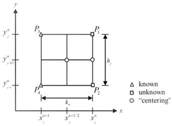
Figure 2.
Net rectangle for difference approximation.
3. Solution Approach
Due to these transformations, the first derivative in the x-direction can be written as shown below.
Moreover, the points on the rectangle are defined as shown below.
Now, We for linearization to Equations (16)–(20).
Moreover, the boundary condition becomes as shown below.
Equations (23)–(29) can be reduced to what follows.
Ri is defined in the Appendix A. Furthermore, the steps required to solve Equations (31)–(37) are also explained in Appendix A; thus, we obtain the following equations.
Similarly, we apply the operator to the boundary equation, which becomes as shown below.
The system of linearized Equations (38)–(41) is transformed into three diagonal block matrices, which can be written as shown.
System (43), by block elimination, can be written as shown.
where are defined as follows.
where [I] is of order 7, known as the identity matrix, and and are also of the order of 7 × 7 matrices.
The elements of L and U can be written as follows.
By Equation (46), Equation (43) becomes as shown.
If , then Equation (50) becomes as shown.
where the following applies.
where is a column matrix of order 7 and can be determined by forward sweep.
Once W is determined, with the help of backward sweep, we find out the solution.
Since is found, we have the approximated solution of the required system (43). The problem is solved using MATLAB coded as given in Appendix B.
4. Outcomes and Discussions
In Figure 3, Figure 4, Figure 5, Figure 6, Figure 7 and Figure 8, the comparisons ofthe thermophoresis parameter and Brownian motion are shown with the help of graphs. It is clear from Figure 3 that with the increases in the thermophoresis parameter (Nt) and Brownian motion (Nb), skin friction increases. The terms of Brownian motion and thermophoresis parameter are inversely related to the viscosity of the fluid. Furthermore, skin friction is related to the friction between the surface and the fluid flow near the surface. So, with the increases in the Brownian motion and thermophoresis viscosity of the fluid and the decrease in the motion of the fluid, skin friction increases as a result. In Figure 4, the Nusselt number is discussed. The Nusselt number is related to the rate of heat transfer of the fluid; moreover, with the increase in thermophoresis, the temperature of the fluid increases, and the fluid easily transfers heat. Therefore, with the increase in the thermophoresis parameter, the Nusselt number increases. Moreover, the Brownian motion parameter (Nb) is related to the concentration of the mass particles. So, with the increase in Brownian motion, the Nusselt number decreases. In Figure 5, the Sherwood number results are reported. The Sherwood number decreases as the thermophoresis number increases; however, for Brownian motion, the Sherwood number increases, as it is related to the mass concentration of the fluid. In Figure 6, the concentration profile results are reported. As the thermophoresis parameter (Nt) and the Brownian motion parameter are enhanced, the concentration profile increases, but the trend becomes opposite when the graph approaches the lowest point.
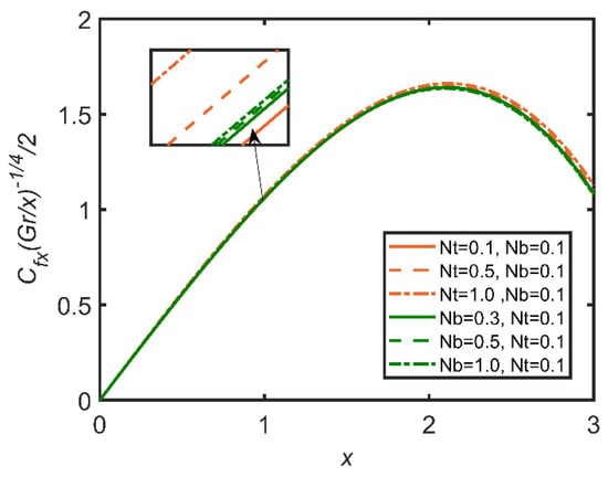
Figure 3.
Comparison for skin friction against x.
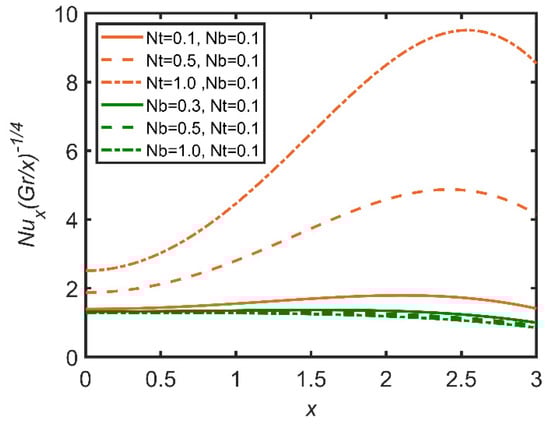
Figure 4.
Comparison for Nusselt number against x.
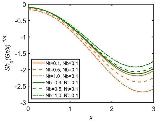
Figure 5.
Comparison for Sherwood number against x.
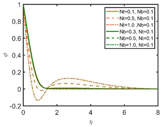
Figure 6.
Comparison for concentration profile against .
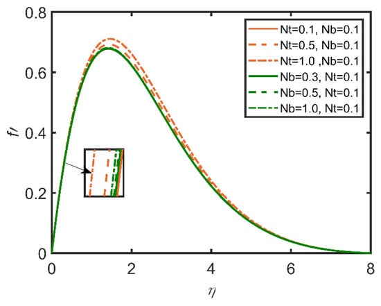
Figure 7.
Comparison for velocity profile against .
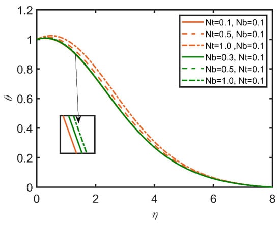
Figure 8.
Comparison for temperature profile against .
In Figure 9, Figure 10, Figure 11, Figure 12, Figure 13 and Figure 14, the comparisons of the buoyancy ratio and the Prandtl number are reported with the help of graphs. In Figure 9, the increase in the buoyancy ratio makes the fluid become less dense and flow easily. Therefore, skin friction increases. However, the Prandtl number decreases, as the Prandtl number is directly related with the viscosity of the fluid. In Figure 11, the Sherwood number increases with the increase in the buoyancy ratio, and as the Prandtl number increases, the Sherwood number decreases. It is due to the increase in the mass flow rate of the concentration of the fluid. In Figure 13, the velocity profile shows that with the increases in the Prandtl number and the buoyancy ratio, the velocity profile becomes smaller. This effect is due to viscosity, which becomes high with the increases in the Prandtl number and the buoyancy ratio. In Figure 14, the temperature profile shows that by increasing the Prandtl number and the buoyancy ratio, we lower the temperature profile; therefore, with the increases in the Prandtl number and the buoyancy ratio, the density of the fluid diminishes.
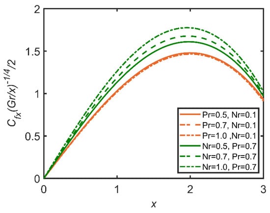
Figure 9.
Comparison for skin friction against x.
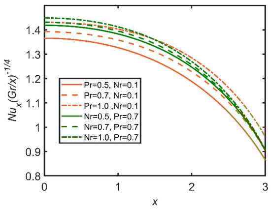
Figure 10.
Comparison for Nusselt number profile against x.
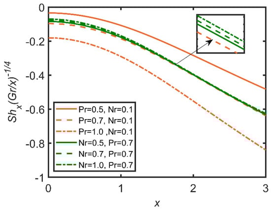
Figure 11.
Comparison for Sherwood number against x.
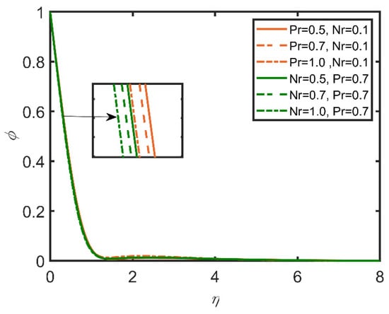
Figure 12.
Comparison for concentration profile against .
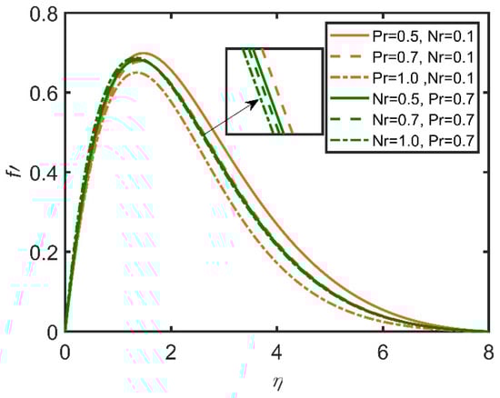
Figure 13.
Comparison for velocity profile against .
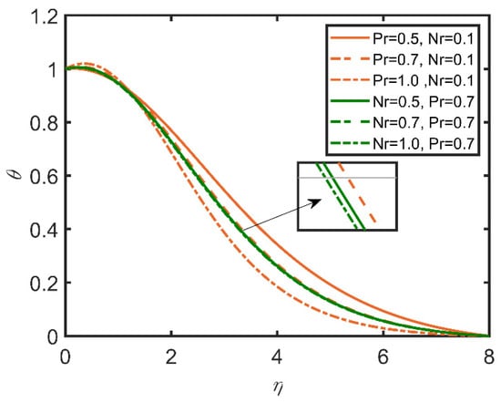
Figure 14.
Comparison for temperature profile against .
In Figure 15, Figure 16, Figure 17, Figure 18, Figure 19 and Figure 20, the comparisons of the heat generation and radiation parameters are reported. In Figure 15, skin friction increases with the increases in the heat generation effect and the radiation parameter. This effect is due to the increase in the temperature of the fluid caused by the increases in these parameters. The fluid becomes less dense, and the friction between the fluid and surface diminishes, so skin friction increases. The same trend can be seen for the Nusselt number by increasing heat generation in Figure 16; however, with the increase in radiation, the Nusselt number decreases, as the radiation parameter is related to the ambient temperature, so when radiation increases, the ambient temperature also increases; therefore, the rate of heat transfer flow from the fluid to the ambient temperature decreases. Hence, the Nusselt number decreases. In Figure 17, the Sherwood number decreases with the increase in heat generation, as the heat generation parameter is inversely related to the concentration of nanoparticles. Hence, the Sherwood number decreases. In Figure 18, the same can be observed, whereby the concentration profile decreases as heat generation increases. In Figure 19, the velocity profile increases as heat generation and radiation increase. This effect is due to the increases in heat generation and radiation, whereby the fluid becomes less dense, and the fluid flows easily. In Figure 20, it is obvious that with the increases in heat generation and radiation, the temperature profile increases, as it rises the temperature of the fluid. So, the temperature profile increases.
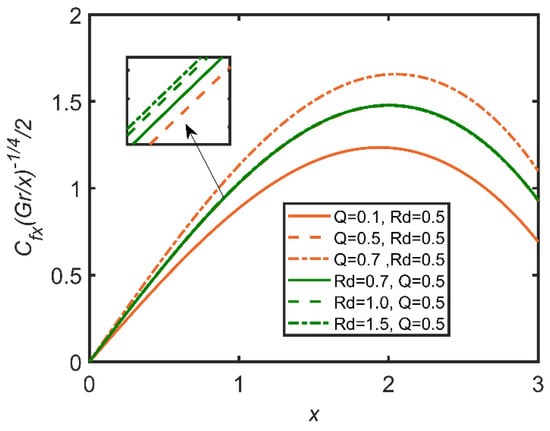
Figure 15.
Comparison for skin friction against x.
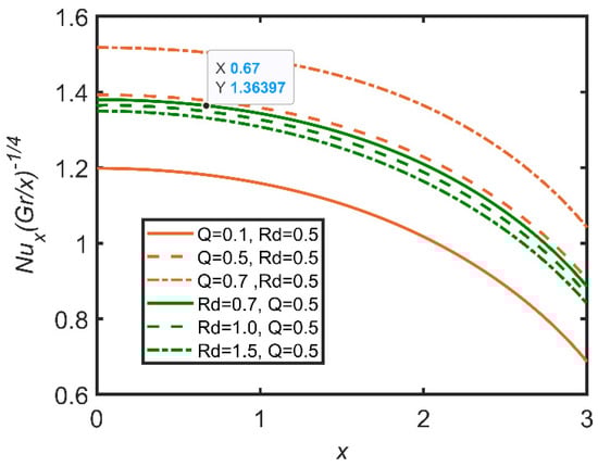
Figure 16.
Comparison for Nusselt number against x.
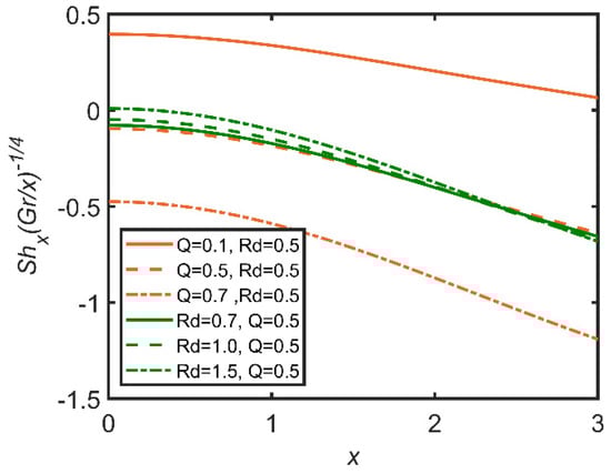
Figure 17.
Comparison for Sherwood number against x.
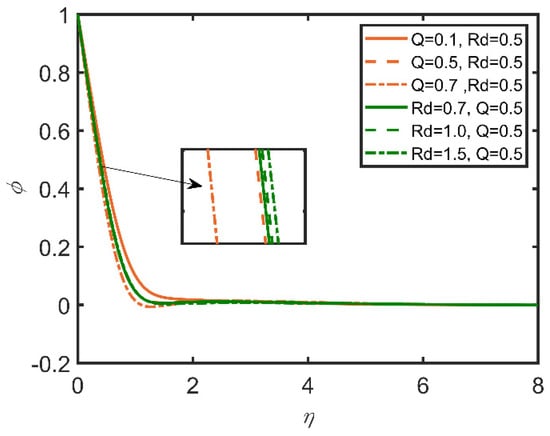
Figure 18.
Comparison for concentration profile against .
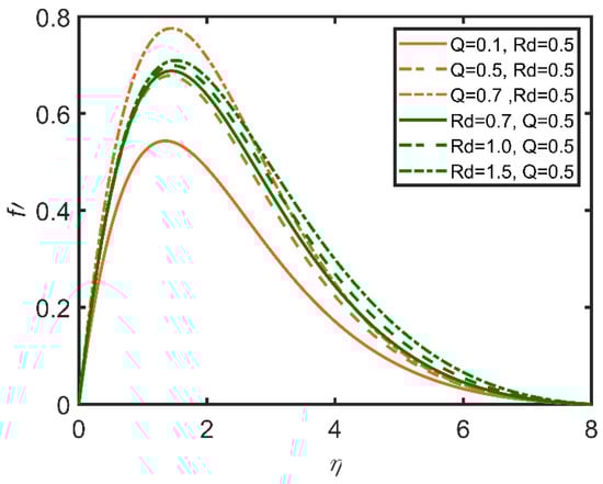
Figure 19.
Comparison for velocity profile against .
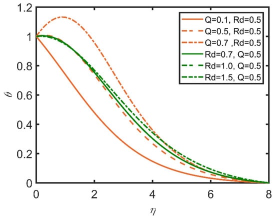
Figure 20.
Comparison for temperature profile against .
In Figure 21, Figure 22 and Figure 23, the comparisons of the effects of Joule heating and the magnetic parameter on the fluid are reported. In Figure 21, with the increase in Joule heating, skin friction increases. This effect is because Joule heating is inverse to the density of the fluid, so the fluid becomes frictionless as Joule heating increases. Moreover, the magnetic parameter lowers skin friction, because the magnetic parameter is directly related to density. Therefore, the greater the magnetic parameter is, the denser the fluid is, and the friction between the surface and the fluid layer becomes high. In Figure 22, the Joule heating effect enhances the Nusselt number, as it is inversely related to the concentration of nanoparticles as well as the temperature difference between the fluid and the ambient temperature; therefore, the rate of heat transfer becomes dominant. The opposite case is verified for the magnetic parameter, whose increase decreases the Nusselt number.
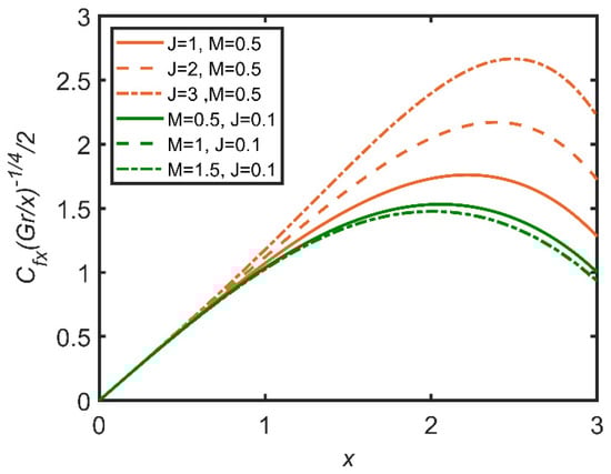
Figure 21.
Comparison for skin friction against x.
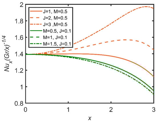
Figure 22.
Comparison for Nusselt number against x.
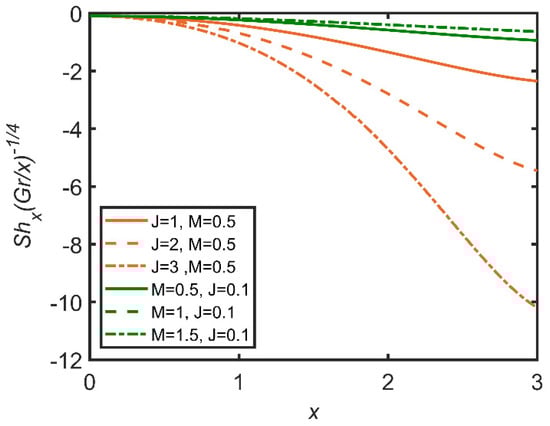
Figure 23.
Comparison for Sherwood number against x.
In Figure 24, Figure 25 and Figure 26, the comparisons of the Lewis number and Eckert number are reported with the help of graphs. In Figure 24, skin friction decreases with the increase in the Lewis number, as it is directly proportional to fluid viscosity. Therefore, the friction between the surface and the fluid increases as a result, as skin friction is enhanced by the increase in the Lewis number. Furthermore, the Eckert number enhances skin friction, as the Eckert number is directly related to the Grashof number of nanoparticles. So, the fluid flow becomes dense. Therefore, skin friction increases. In Figure 25, as the Lewis number is directly related to viscosity, the Nusselt number increases as the Lewis number and the Eckert number both increase, so the rate of heat transfer becomes easier. The Eckert number increases the Grashof number; therefore, the Nusselt number also increases. In Figure 26, the Sherwood number decreases as the Eckert number and the Lewis number increase.
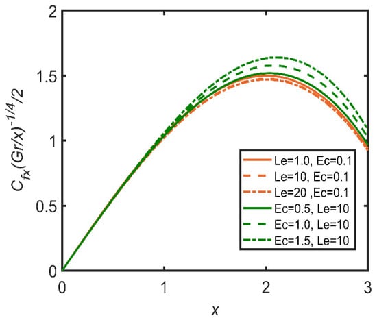
Figure 24.
Comparison for skin friction against x.
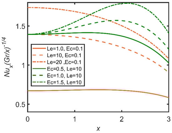
Figure 25.
Comparison for Nusselt number against x.
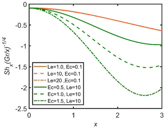
Figure 26.
Comparison for Sherwood number against x.
5. Conclusions
The effects of radiation, heat generation, and magnetic hydrodynamic properties imposed on a nanofluid with a steady, incompressible, natural-convection flow over the horizontally circular form of a cylinder are numerically determined by the very efficient finite element method known as the Keller box method. Buoyancy force and thermophoresis effects are embedded in the nanofluid, and the resultant highly non-linear partial differential equations, including continuity, momentum, energy, and concentration equations, for the mass of nanofluid particles present in the fluid are solved numerically. Then, the governing equations are transformed into their non-dimensional forms with the help of suitable stream functions. The numerical solution is obtained with the help of an implicit finite difference scheme in MATLAB, and the following results are obtained:
- It can be predicted from the graph that the Eckert number increases; then, the Nusselt number increases, but the Sherwood number decreases. This effect is due to the increases in the volume of the nanofluid particles and in the Nusselt number. Furthermore, it does not affect the velocity, concentration, or temperature profile;
- The increases in Brownian motion and buoyancy ratio increase the Nusselt number due to an increase in the volume ratio of the nanoparticles, and rate of heat transfer is enhanced by the increase in the mass ratio;
- The magnetic parameter reduces the Sherwood number and the Nusselt number due to the effects of the movement of the nanoparticles, which is reduced with the increase in the magnetic parameter;
- Heat generation also decreases the Nusselt number, as the rate of heat transfer is reduced due to the reduction in the temperature difference between the wall of the cylinder and the nanofluid.
Author Contributions
Formal analysis, J.A. and M.S.A.; Investigation, A.Z. and M.M. All authors have read and agreed to the published version of the manuscript.
Funding
This research received no external funding.
Institutional Review Board Statement
Not applicable.
Informed Consent Statement
Not applicable.
Data Availability Statement
Not applicable.
Conflicts of Interest
The authors declare no conflict of interest.
Nomenclature
| k | Thermal conductivity (W/mK) |
| DB | Brownian diffusion coefficient (m2/s) |
| a | Radius of the horizontal circular circle (m) |
| Velocity of the fluid at the boundary layer (m/s) | |
| Le | Lewis number (dimensionless number) |
| g | Acceleration due to gravity (m/s2) |
| Gr | Grashof number (dimensionless number) |
| Dimensional and components of velocity (dimensionless number) | |
| u, v | Dimensionless x and y components of velocity (dimensionless number) |
| Nb | Brownian motion parameter (kgm3/s4) |
| Dr | Thermophoretic diffusion coefficient (m2/s K) |
| T | Temperature of the fluid in the boundary layer (K) |
| Temperature of the ambient fluid (K) | |
| Cartesian coordinates (dimensionless number) | |
| x, y | Coordinates in the direction along and normal to surface (dimensionless number) |
| Nu | Local Nusselt Number (dimensionless number) |
| f | Dimensionless stream function (dimensionless number) |
| Nt | Thermophoresis parameter (kgm3/s4K) |
| Nr | Buoyancy ratio (dimensionless number) |
| Pr | Prandtl number (dimensionless number) |
| U | Reference velocity (m/s) |
| Cp | Specific heat term at constant pressure (J/kg⋅K) |
| Local skin friction coefficient (dimensionless number) | |
| Tw | Temperature at the surface (K) |
| Radiative heat flux (w/m2) | |
| C | Nano particle volume fraction (dimensionless number) |
| Nano fluid volume fraction outside the boundary layer (dimensionless number) | |
| Heat flux at the surface (W/m2) | |
| Nanoparticle-concentration expansion coefficient outside the boundary layer (mol/m3) | |
| Rd | Radiation parameter (W/m2) |
| Strength of magnetic field (A/m) | |
| Source term of heat generation (J) | |
| Ec | Eckert number (dimensionless number) |
| J | Joule heating parameter (A2.ohm.s) |
| M | Magnetic parameter (dimensionless number) |
| Q | Heat generation parameter (J) |
| Greek Symbols | |
| α | amplitude of the wavy surface (m) |
| β | volumetric coefficient of thermal expansion (1/K) |
| μ | viscosity of the fluid (kg/m s) |
| ψ | stream function (dimensionless number) |
| σ(x) | surface profile function (dimensionless number) |
| σ | Stefan Boltzman constant ((W/m 2 K 4) |
| η | non-dimensional similarity variable (dimensionless number) |
| τ | shear stress (N/m2) |
| reference kinematic viscosity (m2/s) | |
| θ | dimensionless temperature function (dimensionless number) |
| dynamic viscosity of the ambient fluid (N s/m2) | |
| f | non-dimensional nanoparticle volume fraction (dimensionless number) |
| ρ | density of the fluid (kg/m3) |
| nanoparticle mass density (kg/m3) | |
| fluid velocity outside the boundary layer (m/s) | |
| fluid density (kg/m3) | |
| electrical conductivity (S/m) | |
| scattering coefficient (1/m) | |
| heat capacity of the fluid (J/kg K) | |
| αr | Rosseland mean extinction coefficient (1/m) |
Appendix A
This section shows the solution approaches and the explanation of Equations from (31) to (42).
to Equations (31)–(37).
where the below apply.
We solve Equation (36).
where the below apply.
We solve Equation (37).
where the below apply.
Appendix B
Listing A1: This section shows the MATLAB code used to solve the governed problem.
clear all;clc;
% Problem: Free Convection on a Horizontal Circular Cylinder in a
% nanofluid with Viscous Dissipation
%%%%%%%%%%%%%%%%%%%%%%%%%%%%%%%%%%%%%%%%%%%%%%%%%%%%%%%%%%%%%%%%%%%%
% This Matlab® program solves the problem of laminar free convection
% boundary layer flow on horizontal circular cylinder in a
% nanofluid with viscous dissipation using the Keller-box method
%%%%%%%%%%%%%%%%%%%%%%%%%%%%%%%%%%%%%%%%%%%%%%%%%%%%%%%%%%%%%%%%%%%%%
% The answer displayed in the result sheet will be started from
% number 1 instead of 0
%%%%%%%%%%%%%%%%%%%%%%%%%%%%%%%%%%%%%%%%%%%%%%%%%%%%%%%%%%%%%%%%%%%%%
% Data input
xend = 3;
delx = 0.005;
blt = 8;
deleta = 0.01;
nx = (xend/delx) + 1; np = (blt/deleta) + 1;
pr = 0.7;
ec = 1.5;
J = 0.1;
nt = 0.1;
nb = 0.5;
le = 10;
Nr = 0.1;
M = 0.5;
Q = 0.5;
Rd = 0.5;
x(1) = 0.0; B(1) = 1.0;
for i = 2:nx
x(i) = x(i−1) + delx;
xx(i) = x(i)/(x(i) − x(i−1));
B(i) = sin(x(i))/x(i);
end
for i = 1:nx
stop = 1.0; k = 1;
while stop > 0.00001
eta(1,1) = 0.0;
for j = 2:np
eta(j,1) = eta(j−1,1) + deleta;
end
% the initial value for velocity and temperature profile (f,u,v,s,t,g,p)
etanpq = eta(np,1)/12;
etau15 = 1/eta(np,1);
for j = 1:np
deta(j,k) = deleta;
etab = eta(j,1)/eta(np,1);
etab1 = etab^2;
etab2 = (1 − etab)^2;
if i == 1
f(j,1,i) = etanpq * etab1 * (6 − 8 * etab + 3 * etab1);
u(j,1,i) = etab * etab2;
v(j,1,i) = etau15 * (1 − 4 * etab + 3 * etab1);
s(j,1,i) = etab2;
t(j,1,i) = 2 * etau15 * (etab − 1);
g(j,1,i) = etab2;
p(j,1,i) = 2 * etau15 * (etab − 1);
else
f(j,1,i) = ff(j);
u(j,1,i) = uu(j);
v(j,1,i) = vv(j);
s(j,1,i) = ss(j);
t(j,1,i) = tt(j);
g(j,1,i) = gg(j);
p(j,1,i) = pp(j);
end
end
% To define the coefficients of the linearized equations
for j = 2:np
% Previous station
if i == 1
cfb(j,i) = 0.0; cub(j,i) = 0.0; cvb(j,i) = 0.0;
csb(j,i) = 0.0; ctb(j,i) = 0.0;
cgb(j,i) = 0.0; cpb(j,i) = 0.0;
cuub(j,i) = cub(j,i);
cttb(j,i) = ctb(j,i);
cvvb(j,i) = cvb(j,i);
cfvb(j,i) = cfb(j,i) * cvb(j,i);
cptb(j,i) = cpb(j,i) * ctb(j,i);
cftb(j,i) = cfb(j,i) * ctb(j,i);
cusb(j,i) = cub(j,i) * csb(j,i);
cfpb(j,i) = cfb(j,i) * cpb(j,i);
cgub(j,i) = cgb(j,i) * cub(j,i);
cdervb(j,i) = 0.0; cdertb(j,i) = 0.0; cderpb(j,i) = 0.0;
else
cfb(j,i) = ffb(j); cub(j,i) = uub(j); cvb(j,i) = vvb(j);
csb(j,i) = ssb(j); ctb(j,i) = ttb(j);
cgb(j,i) = ggb(j); cpb(j,i) = ppb(j);
cuub(j,i) = cub(j,i);
cttb(j,i) = ctb(j,i);
cvvb(j,i) = cvb(j,i);
cfvb(j,i) = cfb(j,i) * cvb(j,i);
cptb(j,i) = cpb(j,i) * ctb(j,i);
cftb(j,i) = cfb(j,i) * ctb(j,i);
cusb(j,i) = cub(j,i) * csb(j,i);
cfpb(j,i) = cfb(j,i) * cpb(j,i);
cgub(j,i) = cgb(j,i) * cub(j,i);
cdervb(j,i) = ddervb(j); cdertb(j,i) = ddertb(j);
cderpb(j,i) = dderpb(j);
end
% Present station (centered-difference derivatives)
% Eqs. (4.10)-(4.13)
fb(j,k,i) = 0.5 * (f(j,k,i) + f(j−1,k,i));
ub(j,k,i) = 0.5 * (u(j,k,i) + u(j−1,k,i));
vb(j,k,i) = 0.5 * (v(j,k,i) + v(j−1,k,i));
sb(j,k,i) = 0.5 * (s(j,k,i) + s(j−1,k,i));
tb(j,k,i) = 0.5 * (t(j,k,i) + t(j−1,k,i));
gb(j,k,i) = 0.5 * (g(j,k,i) + g(j−1,k,i));
pb(j,k,i) = 0.5 * (p(j,k,i) + p(j−1,k,i));
uub(j,k,i) = ub(j,k,i)^2;
ttb(j,k,i) = tb(j,k,i)^2;
vvb(j,k,i) = vb(j,k,i)^2;
fvb(j,k,i) = fb(j,k,i) * vb(j,k,i);
ftb(j,k,i) = fb(j,k,i) * tb(j,k,i);
usb(j,k,i) = ub(j,k,i) * sb(j,k,i);
fpb(j,k,i) = pb(j,k,i) * fb(j,k,i);
ptb(j,k,i) = pb(j,k,i) * tb(j,k,i);
gub(j,k,i) = gb(j,k,i) * ub(j,k,i);
dervb(j,k,i) = (v(j,k,i) − v(j−1,k,i))/deta(j,k);
dertb(j,k,i) = (t(j,k,i) − t(j−1,k,i))/deta(j,k);
derpb(j,k,i) = (p(j,k,i) − p(j−1,k,i))/deta(j,k);
% Coefficients of the difference momentum equation
% Eq. (4.40)
a1(j,k) = 1.0 + (deta(j,k) + (0.5 * (1.0 + xx(i)) * fb(j,k,i)−0.5 * xx(i) * cfb(j,i)));
a2(j,k) = −1.0 + (deta(j,k) + (0.5 * (1.0 + xx(i)) * fb(j,k,i)−0.5 * xx(i) * cfb(j,i)));
a3(j,k) = 0.5 * deta(j,k) * (1.0 + xx(i)) * (vb(j,k,i)+ cvb(j,i));
a4(j,k) = a3(j,k);
a5(j,k) = −1.0 * deta(j,k) * ((1 + xx(i)) * ub(j,k,i))+0.5*deta(j,k)*M*x(i);
a6(j,k) = a5(j,k);
a7(j,k) = B(i) * 0.5 * deta(j,k);
a8(j,k) = a7(j,k);
a9(j,k) = B(i) * 0.5 * deta(j,k) * Nr;
a10(j,k) = a9(j,k);
% Coefficients of the difference energy equation
% Eq. (4.41)
b1(j,k) = (1.0/pr)*(1+(4/3)*Rd) + deta(j,k) + ((1.0 + xx(i)) * 0.5 *fb(j,k,i) − xx(i) * 0.5 * cfb(j,i)+ nb * 0.5 *pb(j,k,i)+nt * tb(j,k,i));
b2(j,k) = (−1.0/pr)*(1+(4/3)*Rd) + deta(j,k) + ((1.0 + xx(i)) * 0.5 *fb(j,k,i) − xx(i) * 0.5 * cfb(j,i)+ nb * 0.5 *pb(j,k,i)+nt * tb(j,k,i));
b3(j,k) = 0.5 * deta(j,k) * ((1 + xx(i)) * tb(j,k,i)+xx(i) * ctb(j,i));
b4(j,k) = b3(j,k);
b5(j,k) = −0.5 * deta(j,k) * xx(i) * (ub(j,k,i) + cub(j,i))+Q*0.5*deta(j,k);
b6(j,k) = b5(j,k);
b7(j,k) = deta(j,k) * 0.5 * xx(i) * (- sb(j,k,i) + csb(j,i))+J*deta(j,k)*ub(j,k,i)*(x(i))^2;
b8(j,k) = b7(j,k);
b9(j,k) = deta(j,k) * 0.5 * nb * tb(j,k,i);
b10(j,k) = b9(j,k);
b11(j,k) = deta(j,k)*vb(j,k,i) * ec * (x(i))^2 + 0.5* deta(j,k)*cvb(j,i) * ec * (x(i))^2;
b12(j,k) = b11(j,k);
% Coefficients of the difference angular momentum equations
% Eq. (4.42)
c1(j,k) = 1.0 + (le * deta(j,k) + 0.5) * (((1 + xx(i))*fb(j,k,i)) - (xx(i) * cfb(j,i)));
c2(j,k) = c1(j,k) - (2.0);
c3(j,k) = (nt/nb);
c4(j,k) = - c3(j,k);
c5(j,k) = 0.5 * deta(j,k) + le * ((1.0 + xx(i)) * pb(j,k,i)+xx(i) * cpb(j,i));
c6(j,k) = c5(j,k);
c7(j,k) = −0.5 * le * deta(j,k) * xx(i) * (ub(j,k,i) + cub(j,i));
c8(j,k) = c7(j,k);
c9(j,k) = 0.5 * deta(j,k) * le * xx(i) * (cgb(j,i) - gb(j,k,i));
c10(j,k) = c9(j,k);
% Expressions of Rj
R1 = −1.0 * deta(j,k) + (cdervb(j,i) + cfvb(j,i) - cuub(j,i)+B(i) * (csb(j,i) + Nr * cgb(j,i)) - (xx(i) * cfvb(j,i))+(xx(i) * cuub(j,i))+M*x(i)*cub(j,i));
R2 = −1.0 * deta(j,k) + (cdertb(j,i) * (1.0/pr)*(1+(4/3)*Rd)+(1 - xx(i))* cftb(j,i) + nb * cptb(j,i) + nt * cttb(j,i)+(xx(i) * cusb(j,i))+ (0.5 * ec * ((xx(i) * delx)^2)*cvvb(j,i))+Q*csb(j,i)+J*cuub(j,i)*(x(i))^2);
R3 = −1.0 * deta(j,k) + (cderpb(j,i) + (nt/nb) * cdertb(j,i)+le * cfpb(j,i) - le * xx(i) * cfpb(j,i) + le * xx(i)*cgub(j,i));
% Expressions of rj−1/2
% Eq. (4.43)
r1(j,k) = f(j−1,k,i) - f(j,k,i) + deta(j,k) * ub(j,k,i);
r2(j,k) = u(j−1,k,i) - u(j,k,i) + deta(j,k) * vb(j,k,i);
r3(j,k) = s(j−1,k,i) - s(j,k,i) + deta(j,k) * tb(j,k,i);
r4(j,k) = g(j−1,k,i) - g(j,k,i) + deta(j,k) * pb(j,k,i);
r5(j,k) = v(j−1,k,i) - v(j,k,i) - deta(j,k) * (1 + xx(i))*(fvb(j,k,i) - uub(j,k,i)) - deta(j,k) * (B(i) * sb(j,k,i)+B(i) * Nr * gb(j,k,i) + xx(i) * fb(j,k,i) * cvb(j,i)-xx(i) * cfb(j,i) * vb(j,k,i)-M*ub(j,k,i)*x(i)) + R1;
r6(j,k) = (1.00/pr)*(1+(4/3)*Rd) * (t(j−1,k,i) - t(j,k,i)) - (1.0+xx(i))* deta(j,k) * ftb(j,k,i) - deta(j,k) * nb * ptb(j,k,i)-nt * deta(j,k) * ttb(j,k,i) + xx(i) * deta(j,k)*usb(j,k,i) + xx(i) * deta(j,k) * sb(j,k,i)*cub(j,i) - xx(i)* deta(j,k)*csb(j,i) * ub(j,k,i) + xx(i) * deta(j,k) * tb(j,k,i)*cfb(j,i) - xx(i) * deta(j,k) * ctb(j,i) * fb(j,k,i)-((xx(i) * delx)^2) * ec * deta(j,k) * vvb(j,k,i)-((xx(i) * delx)^2) * ec * deta(j,k) * vb(j,k,i) * cvb(j,i)-Q*deta(j,k)*sb(j,k,i)-J*deta(j,k)*uub(j,k,i)*(x(i))^2+R2;
r7(j,k) = (p(j−1,k,i) - p(j,k,i)) + (nt/nb) * (t(j−1,k,i)-t(j,k,i)) - le * deta(j,k) * (1 + xx(i)) * fpb(j,k,i)+xx(i) * deta(j,k) * le * gub(j,k,i) - xx(i) * le * deta(j,k)*ub(j,k,i) * cgb(j,i) + xx(i) * le * deta(j,k) * gb(j,k,i) * cub(j,i) + xx(i) * le * deta(j,k) * pb(j,k,i) * cfb(j,i)-xx(i) * le * deta(j,k) * fb(j,k,i) * cpb(j,i) + R3;
end
% Obtain the matrices
% Eqs. (4.47)-(4.50)
a{2,k} = [ 0 0 0 1 0 0 0;
−0.5*deta(2,k) 0 0 0 −0.5*deta(2,k) 0 0;
0 −0.5*deta(2,k) 0 0 0 −0.5*deta(2,k) 0;
0 0 −0.5*deta(2,k) 0 0 0 −0.5*deta(2,k);
a2(2,k) 0 0 a3(2,k) a1(2,k) 0 0;
b12(2,k) b2(2,k) b10(2,k) b3(2,k) b11(2,k) b1(2,k) b9(2,k);
0 c4(2,k) c2(2,k) c5(2,k) 0 c3(2,k) c1(2,k) ];
for j = 3:np
a{j,k} = [ −0.5*deta(j,k) 0 0 1 0 0 0;
−1 0 0 0 −0.5*deta(j,k) 0 0;
0 0 −1 0 0 −0.5*deta(j,k) 0;
0 −1 0 0 0 0 −0.5*deta(j,k);
a6(j,k) a10(j,k) a8(j,k) a3(j,k) a1(j,k) 0 0;
b8(j,k) 0 b6(j,k) b3(j,k) b11(j,k) b1(j,k) b9(j,k);
c10(j,k) c8(j,k) 0 c5(j,k) 0 c3(j,k) c1(j,k) ];
b{j,k} = [ 0 0 0 −1 0 0 0;
0 0 0 0 −0.5*deta(j,k) 0 0;
0 0 0 0 0 −0.5*deta(j,k) 0;
0 0 0 0 0 0 −0.5*deta(j,k);
0 0 0 a4(j,k) a2(j,k) 0 0;
0 0 0 b4(j,k) b12(j,k) b2(j,k) b10(j,k);
0 0 0 c6(j,k) 0 c4(j,k) c2(j,k) ];
end
for j = 2:np
c{j,k} = [ −0.5*deta(j,k) 0 0 0 0 0 0;
1 0 0 0 0 0 0;
0 0 1 0 0 0 0;
0 1 0 0 0 0 0;
a5(j,k) a9(j,k) a7(j,k) 0 0 0 0;
b7(j,k) 0 b5(j,k) 0 0 0 0;
c9(j,k) c7(j,k) 0 0 0 0 0 ];
end
% The recuesion formulas
% forward sweep
% Eqs. (4.54)-(4.62)
alfa{2,k} = a{2,k};
gamma{2,k} = inv(alfa{2,k}) * c{2,k};
for j = 3:np
alfa{j,k} = a{j,k} - (b{j,k} * gamma{j−1,k});
gamma{j,k} = inv(alfa{j,k}) * c{j,k};
end
for j = 2:np
rr{j,k} = [ r1(j,k); r2(j,k); r3(j,k); r4(j,k); r5(j,k);
r6(j,k); r7(j,k) ];
end
ww{2,k} = inv(alfa{2,k}) * rr{2,k};
for j = 3:np
ww{j,k} = inv(alfa{j,k}) * (rr{j,k} - (b{j,k} * ww{j−1,k}));
end
% backward sweep
% Eqs. (4.63)-(4.64)
delf(1,k) = 0.0; dels(1,k) = 0.0; delu(1,k) = 0.0; delg(1,k) = 0.0;
delu(np,k) = 0.0; dels(np,k) = 0.0; delg(np,k) = 0.0;
dell{np,k} = ww{np,k};
for j = np-1:-1:2
dell{j,k} = ww{j,k} - (gamma{j,k} * dell{j+1,k});
end
delv(1,k) = dell{2,k}(1,1);
delt(1,k) = dell{2,k}(2,1);
delp(1,k) = dell{2,k}(3,1);
delf(2,k) = dell{2,k}(4,1);
delv(2,k) = dell{2,k}(5,1);
delt(2,k) = dell{2,k}(6,1);
delp(2,k) = dell{2,k}(7,1);
for j = np:-1:3
delu(j-1,k) = dell{j,k}(1,1);
delg(j-1,k) = dell{j,k}(2,1);
dels(j-1,k) = dell{j,k}(3,1);
delf(j,k) = dell{j,k}(4,1);
delv(j,k) = dell{j,k}(5,1);
delt(j,k) = dell{j,k}(6,1);
delp(j,k) = dell{j,k}(7,1);
end
% Newton’s method
% Eq.(4.32)
for j = 1:np
f(j,k+1,i) = f(j,k,i) + delf(j,k);
u(j,k+1,i) = u(j,k,i) + delu(j,k);
v(j,k+1,i) = v(j,k,i) + delv(j,k);
s(j,k+1,i) = s(j,k,i) + dels(j,k);
t(j,k+1,i) = t(j,k,i) + delt(j,k);
g(j,k+1,i) = g(j,k,i) + delg(j,k);
p(j,k+1,i) = p(j,k,i) + delp(j,k);
end
% check for convergence of the iterations
% Eq. (4.65)
stop = abs(delv(1,k));
kmax(i) = k;
k = k+1;
end
% Shift profile
for j = 1:np
ff(j) = f(j,k,i); uu(j) = u(j,k,i); vv(j) = v(j,k,i);
ss(j) = s(j,k,i); tt(j) = t(j,k,i);
gg(j) = g(j,k,i); pp(j) = p(j,k,i);
end
for j = 1:np
ffb(j) = fb(j,kmax(i),i);
uub(j) = ub(j,kmax(i),i);
vvb(j) = vb(j,kmax(i),i);
ssb(j) = sb(j,kmax(i),i);
ttb(j) = tb(j,kmax(i),i);
ggb(j) = gb(j,kmax(i),i);
ppb(j) = pb(j,kmax(i),i);
ddervb(j) = dervb(j,kmax(i),i);
ddertb(j) = dertb(j,kmax(i),i);
dderpb(j) = derpb(j,kmax(i),i);
end
% Physical Quantity Interested
% Eq. (4.0)
cf(i) = x(i) * v(1,kmax(i),i);
q(i) = -(1+(4/3)*Rd)*t(1,kmax(i),i);
h(i) = -p(1,kmax(i),i);
[i x(i) cf(i) q(i) h(i)]
end
% Output Figure
aaa = [eta’; g(:,kmax(1))’];
aaa1 = [eta’; s(:,kmax(1))’];
aaa2 = [eta’; u(:,kmax(1))’];
aaa3 = [x; cf];
aaa4 = [x; q];
aaa5 = [x; h];
file1 = fopen(‘g.txt’,’w’);
fprintf(file1,’%12.8f %12.8f\n’,aaa);
fclose(file1);
file2 = fopen(‘s.txt’,’w’);
fprintf(file2,’%12.8f %12.8f\n’,aaa1);
fclose(file2);
file3 = fopen(‘u.txt’,’w’);
fprintf(file3,’%12.8f %12.8f\n’,aaa2);
fclose(file3);
file4 = fopen(‘cf.txt’,’w’);
fprintf(file4,’%12.8f %12.8f\n’,aaa3);
fclose(file4);
file5 = fopen(‘q.txt’,’w’);
fprintf(file5,’%12.8f %12.8f\n’,aaa4);
fclose(file5);
file6 = fopen(‘h.txt’,’w’);
fprintf(file6,’%12.8f %12.8f\n’,aaa5);
fclose(file6);
figure (1)
plot (eta,g(:,kmax(1)))
xlabel(‘\eta’)
ylabel(‘fai(\eta)’)
hold on
figure (2)
plot (eta,s(:,kmax(1)))
xlabel(‘\eta’)
ylabel(‘\theta(\eta)’)
hold on
figure (3)
plot (eta,u(:,kmax(1)))
xlabel(‘\eta’)
ylabel(‘u(\eta)’)
hold on
figure (4)
plot (x,cf)
xlabel(‘x’)
ylabel(‘Skin friction’)
hold on
figure (5)
plot (x,q)
xlabel(‘x’)
ylabel(‘Sherwood number’)
hold on
figure (6)
plot (x,h)
xlabel(‘x’)
ylabel(‘Nusselt number’)
hold off
References
- Blasius, H. Grenzschichten in Flüssigkeiten Mit Kleiner Reibung; Druck von BG Teubner: Leipzig, Germany, 1907. [Google Scholar]
- Merkin, J.H. Free convection boundary layers on cylinders of elliptic cross section. J. Heat Transf. 1977, 99, 453–457. [Google Scholar] [CrossRef]
- Merkin, J.H. Mixed convection from a horizontal circular cylinder. Int. J. Heat Mass Transf. 1977, 20, 73–77. [Google Scholar] [CrossRef]
- Pop, I.; Ingham, D.B. Convective Heat Transfer: Mathematical and Computational Modelling of Viscous Fluids and Porous Media; Elsevier: Oxford, UK, 2001. [Google Scholar]
- Mohamed, M.K.A.; Noar, N.; Salleh, M.Z.; Ishak, A. Free convection boundary layer flow on a horizontal circular cylinder in a nanofluid with viscous dissipation. Sains Malays. 2016, 45, 289–296. [Google Scholar]
- Choi, S.U.; Eastman, J.A. Enhancing Thermal Conductivity of Fluids with Nanoparticles; Argonne National Lab. (ANL): Argonne, IL, USA, 1995. [Google Scholar]
- Zokri, S.M.; Arifin, N.S.; Kasim, A.R.M.; Salleh, M.Z. Free convection boundary layer flow of Jeffrey nanofluid on a horizontal circular cylinder with viscous dissipation effect. J. Adv. Res. Micro Nano Eng. 2020, 1, 1–14. [Google Scholar]
- Hassan, M.; Ellahi, R.; Zeeshan, A.; Bhatti, M.M. Analysis of natural convective flow of non-Newtonian fluid under the effects of nanoparticles of different materials. Proceedings of the Institution of Mechanical Engineers. Part E J. Process Mech. Eng. 2019, 233, 643–652. [Google Scholar] [CrossRef]
- Nisa, Z.U.; Hajizadeh, A.; Nazar, M. Free convection flow of nanofluid over infinite vertical plate with damped thermal flux. Chin. J. Phys. 2019, 59, 175–188. [Google Scholar] [CrossRef]
- Ellahi, R.; Zeeshan, A.; Waheed, A.; Shehzad, N.; Sait, S.M. Natural convection nanofluid flow with heat transfer analysis of carbon nanotubes–water nanofluid inside a vertical truncated wavy cone. Math. Methods Appl. Sci. 2021. [CrossRef]
- Mourad, A.; Aissa, A.; Mebarek-Oudina, F.; Al-Kouz, W.; Sahnoun, M. Natural convection of nanoliquid from elliptic cylinder in wavy enclosure under the effect of uniform magnetic field: Numerical investigation. Eur. Phys. J. Plus 2021, 136, 429. [Google Scholar] [CrossRef]
- Eastman, J.A.; Choi, S.; Li, S.; Yu, W.; Thompson, L.J. Anomalously increased effective thermal conductivities of ethylene glycol-based nanofluids containing copper nanoparticles. Appl. Phys. Lett. 2001, 78, 718–720. [Google Scholar] [CrossRef]
- Das, S.K.; Putra, N.; Thiesen, P.; Roetzel, W. Temperature dependence of thermal conductivity enhancement for nanofluids. J. Heat Transf. 2003, 125, 567–574. [Google Scholar] [CrossRef]
- Hossain, M.A.; Alim, M.A. Natural convection-radiation interaction on boundary layer flow along a thin vertical cylinder. Heat Mass Transf. 1997, 32, 515–520. [Google Scholar] [CrossRef]
- Hossain, M.; Kutubuddin, M.; Pop, I. Radiation-conduction interaction on mixed convection from a horizontal circular cylinder. Heat Mass Transf. 1999, 35, 307–314. [Google Scholar] [CrossRef]
- Elbashbeshy, E.M.; Emam, T.G.; Sayed, E.A.A. Effect of thermal radiation on free convection flow and heat transfer over a truncated cone in the presence of pressure work and heat generation/absorption. Therm. Sci. 2016, 20, 555–565. [Google Scholar] [CrossRef]
- Zeeshan, A.; Shehzad, N.; Abbas, T.; Ellahi, R. Effects of radiative electro-magnetohydrodynamics diminishing internal energy of pressure-driven flow of titanium dioxide-water nanofluid due to entropy generation. Entropy 2019, 21, 236. [Google Scholar] [CrossRef] [Green Version]
- Vajravelu, K.; Hadjinicolaou, A. Heat transfer in a viscous fluid over a stretching sheet with viscous dissipation and internal heat generation. Int. Commun. Heat Mass Transf. 1993, 20, 417–430. [Google Scholar] [CrossRef]
- Molla, M.M.; Hossain, M.A.; Paul, M.C. Natural convection flow from an isothermal horizontal circular cylinder in presence of heat generation. Int. J. Eng. Sci. 2006, 44, 949–958. [Google Scholar] [CrossRef]
- Molla, M.M.; Paul, S.C.; Hossain, M.A. Natural convection flow from a horizontal circular cylinder with uniform heat flux in presence of heat generation. Appl. Math. Model. 2009, 33, 3226–3236. [Google Scholar] [CrossRef]
- Cheng, C.-Y. Natural convection heat transfer from a horizontal isothermal elliptical cylinder with internal heat generation. Int. Commun. Heat Mass Transf. 2009, 36, 346–350. [Google Scholar] [CrossRef]
- Mohamed, M.K.A.; Sarif, N.M.; Kasim, A.R.M.; Noar, N.; Salleh, M.Z.; Ishak, A. Effects of viscous dissipation on free convection boundary layer flow towards a horizontal circular cylinder. ARPN J. Eng. Appl. Sci. 2016, 11, 7258–7263. [Google Scholar]
- Hossain, M.; Das, S.; Pop, I. Heat transfer response of MHD free convection flow along a vertical plate to surface temperature oscillations. Int. J. Non-Linear Mech. 1998, 33, 541–553. [Google Scholar] [CrossRef]
- Wilks, G. Magnetohydrodynamic free convection about a semi-infinite vertical plate in a strong cross field. Z. Angew. Math. Phys. ZAMP 1976, 27, 621–631. [Google Scholar] [CrossRef]
- Azim, N.; Chowdhury, M. MHD-conjugate free convection from an isothermal horizontal circular cylinder with joule heating and heat generation. J. Comput. Methods Phys. 2013, 2013, 180516. [Google Scholar] [CrossRef] [Green Version]
- Azim, N. Effects of viscous dissipation and heat generation on MHD conjugate free convection flow from an isothermal horizontal circular cylinder. SOP Trans. Appl. Phys. 2014, 1, 1–11. [Google Scholar] [CrossRef]
- Ellahi, R.; Hassan, M.; Zeeshan, A. Study of natural convection MHD nanofluid by means of single and multi-walled carbon nanotubes suspended in a salt-water solution. IEEE Trans. Nanotechnol. 2015, 14, 726–734. [Google Scholar] [CrossRef]
- Nazeer, M.; Ali, N.; Javed, T. Numerical simulations of MHD forced convection flow of micropolar fluid inside a right-angled triangular cavity saturated with porous medium: Effects of vertical moving wall. Can. J. Phys. 2019, 97, 1–13. [Google Scholar] [CrossRef]
- Hobiny, A.; Alzahrani, F.; Abbas, I.; Marin, M. The effect of fractional time derivative of bioheat model in skin tissue induced to laser irradiation. Symmetry 2020, 12, 602. [Google Scholar] [CrossRef]
- Marin, M.; Othman, M.; Abbas, I. An extension of the domain of influence theorem for generalized thermoelasticity of anisotropic material with voids. J. Comput. Theor. Nanosci. 2015, 12, 1594–1598. [Google Scholar] [CrossRef]
- Bhatti, M.M.; Marin, M.; Zeeshan, A.; Abdelsalam, S.I. Recent trends in computational fluid dynamics. Front. Phys 2020, 8, 593111. [Google Scholar] [CrossRef]
- Marin, M.; Florea, O. On temporal behaviour of solutions in thermoelasticity of porous micropolar bodies. An. Univ. Ovidius Constanta-Ser. Mat. 2014, 22, 169–188. [Google Scholar] [CrossRef] [Green Version]
- Abouelregal, A.E.; Marin, M. The Response of Nanobeams with Temperature-Dependent Properties Using State-Space Method via Modified Couple Stress Theory. Symmetry 2020, 12, 1276. [Google Scholar] [CrossRef]
- Zeeshan, A.; Majeed, A.; Akram, M.J.; Alzahrani, F. Numerical investigation of MHD radiative heat and mass transfer of nanofluid flow towards a vertical wavy surface with viscous dissipation and Joule heating effects using Keller-box method. Math. Comput. Simul. 2021, 190, 1080–1109. [Google Scholar] [CrossRef]
Publisher’s Note: MDPI stays neutral with regard to jurisdictional claims in published maps and institutional affiliations. |
© 2022 by the authors. Licensee MDPI, Basel, Switzerland. This article is an open access article distributed under the terms and conditions of the Creative Commons Attribution (CC BY) license (https://creativecommons.org/licenses/by/4.0/).