
Singular Spectrum Analysis of Tremorograms for Human Neuromotor Reaction Estimation


Abstract
:1. Introduction
2. Materials and Methods
2.1. Singular Spectrum Decomposition Method
2.2. Classification and Grouping
- The singular values of the trajectory matrix of the L-dimensional representation of the original one-dimensional series.
- A set of singular vectors of the trajectory matrix. Since their elements are ordered by the operator of the series matrix formation, they can be studied as functions of time.
- The set of principal components of the L-dimensional representation. They, as well as their corresponding eigenvectors, form an orthogonal system and can be considered as functions of the number i.
- Time series reconstructed from different sets of principal components .
2.2.1. Visual Analysis by Singular Values
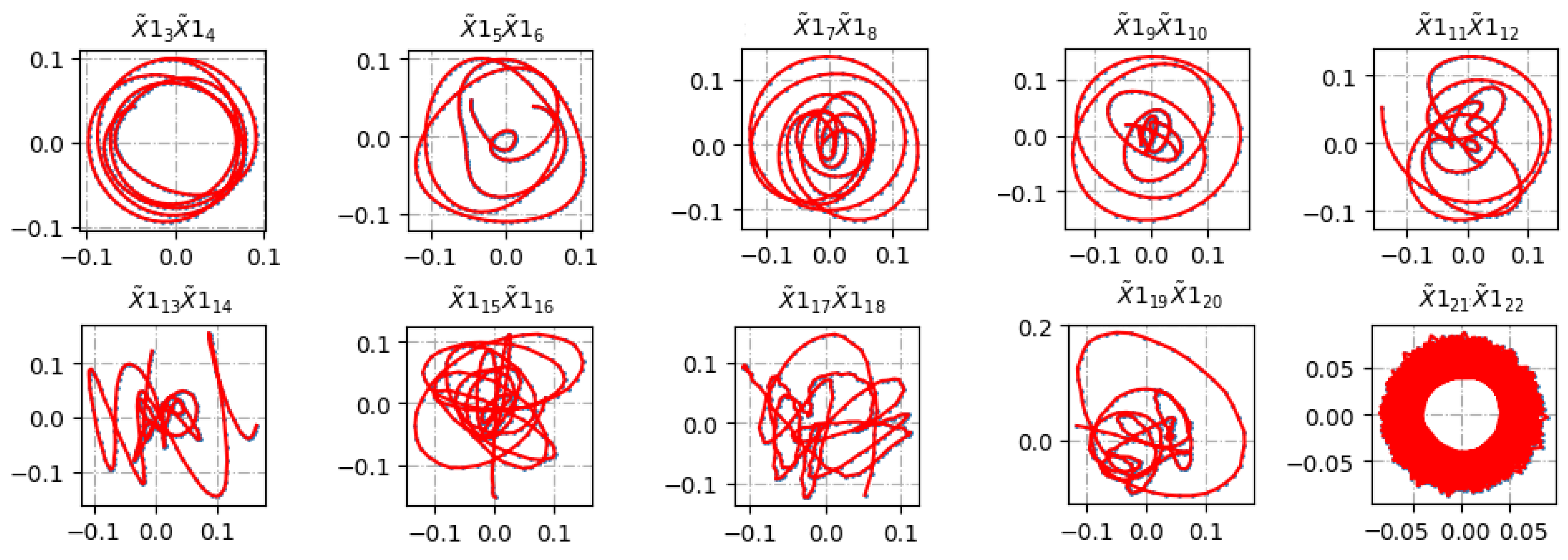
2.2.2. Visual Analysis by Eigenvectors
2.2.3. Classification by Principal Components and Reconstructed Time Series
3. Result
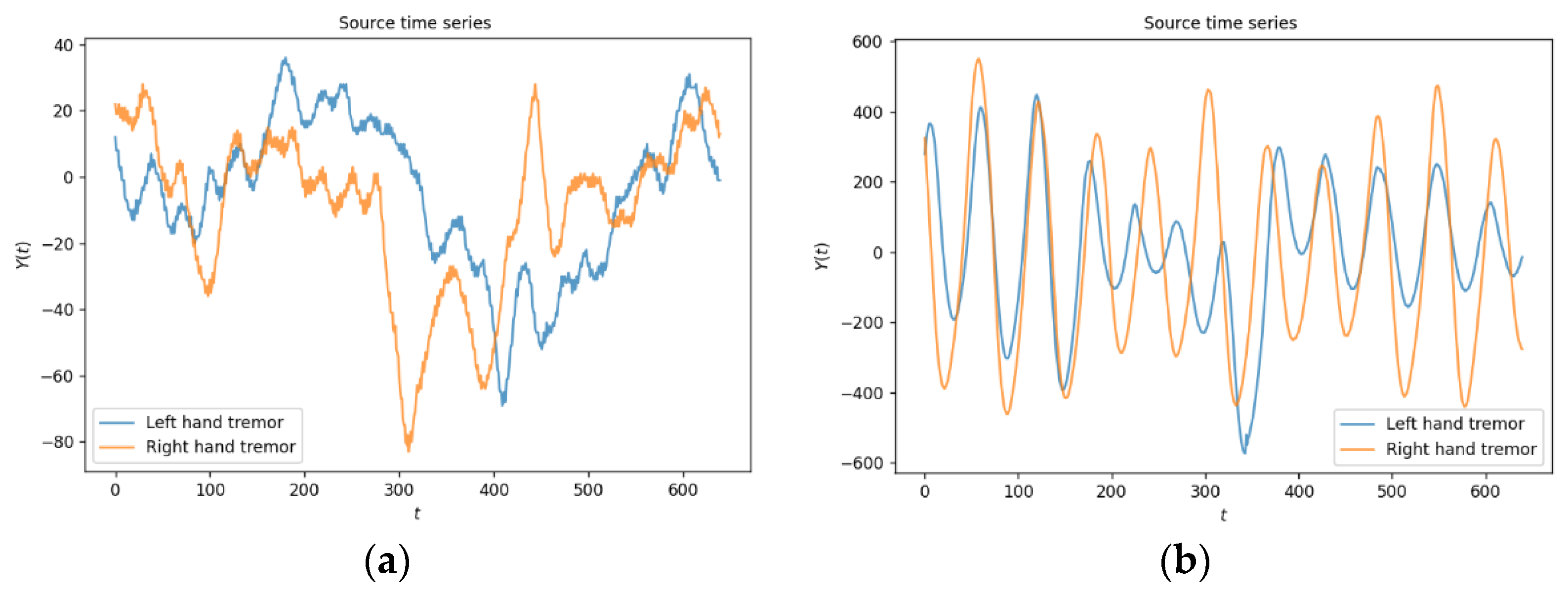
3.1. Data Acquisition
3.2. Singular Spectrum Decomposition of the Original Series
3.3. Classification of Principal Components
| Algorithm 1 Principal component classification algorithm |
| Input: Set of singular values σi Output: Trend, harmonic, and noise sets STEP 1: Calculate the set of logarithms of the singular values σi. |
| STEP 2: Determine the threshold value dd for the distance between logarithms of neighboring singular values considered as pairs, and the scaling factor c for determining the distances between pairs. |
| STEP 3: Analyze sequentially the pairs of neighboring values from the set of logarithms of singular values. If the distance between values in the pair is greater than dd, then the first point is added to the trend set. Else, we assume that the points can form a pair; to identify the pair, go to Step 4. STEP 4: Calculate the distance between the second point of a pair and the one next to it. If the distance is greater than dd*c, then the pair is found. Return to step 3. If the distance is less than dd*c, we assume that the components corresponding to the analyzed singular values and all subsequent ones are noisy. |
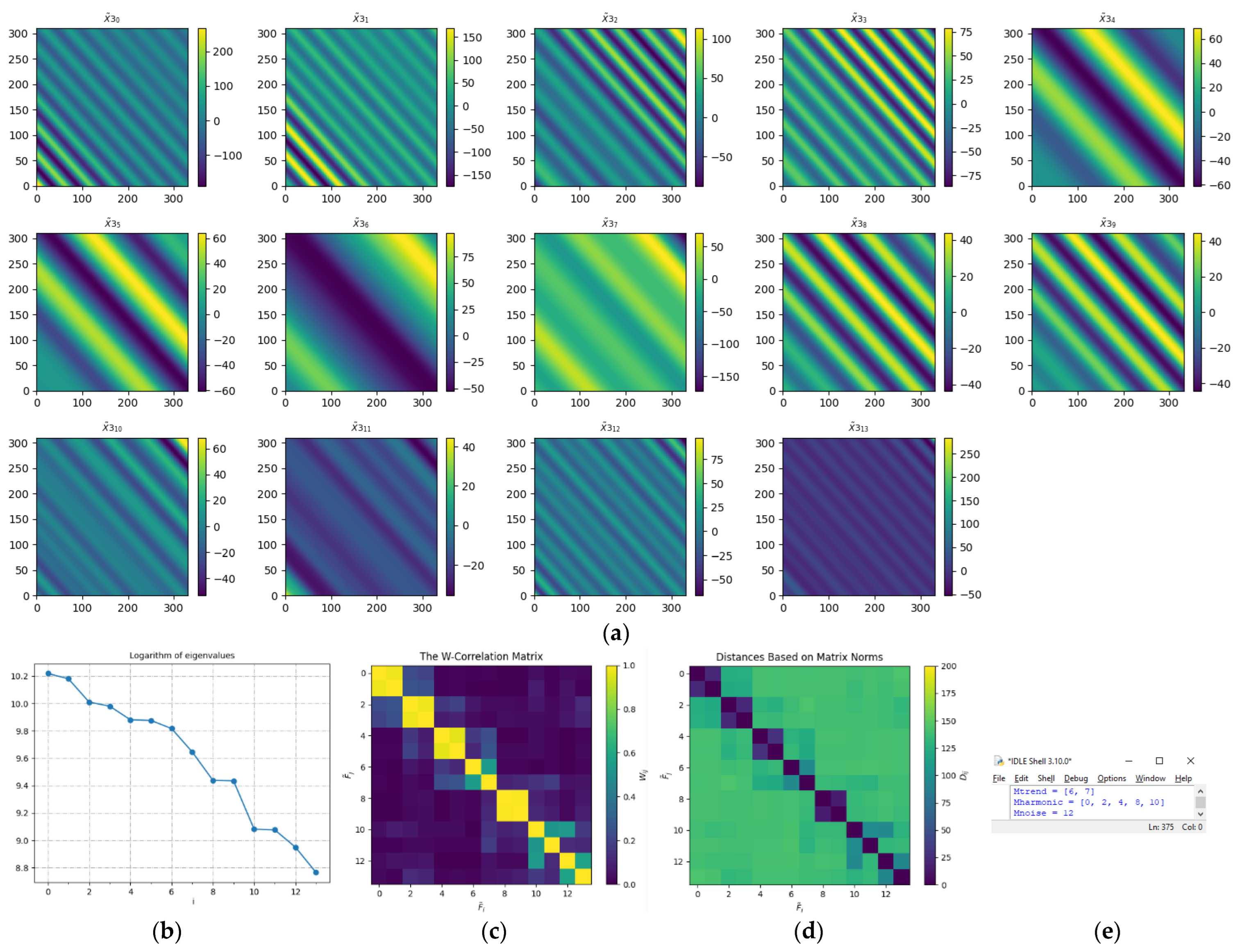
- Trend: σ0, σ1, σ2;
- Harmonic: σ3, σ4; σ5, σ6; σ7, σ8;
- Noise: σ9, and so on.
3.4. Generalized Algorithm for the Analysis of Tremorograms
4. Discussion
5. Conclusions
Author Contributions
Funding
Institutional Review Board Statement
Informed Consent Statement
Data Availability Statement
Conflicts of Interest
Appendix A


References
- Nittari, G.; Savva, D.; Tomassoni, D.; Tayebati, S.K.; Amenta, F. Telemedicine in the COVID-19 Era: A Narrative Review Based on Current Evidence. Int. J. Environ. Res. Public Health 2022, 19, 5101. [Google Scholar] [CrossRef] [PubMed]
- Elkbuli, A.; Ehrlich, H.; McKenney, M. The effective use of telemedicine to save lives and maintain structure in a healthcare system: Current response to COVID-19. Am. J. Emerg. Med. 2021, 44, 468–469. [Google Scholar] [CrossRef] [PubMed]
- Busso, M.; González, M.P.; Scartascini, C. On the Demand for Telemedicine: Evidence from the COVID-19 Pandemic; IDB Working Paper Series; IDP: Washington, DC, USA, 2021. [Google Scholar] [CrossRef]
- Nasiri, K.; Dimitrova, A. The role of telemedicine tools in managing the new chapter of SARS-CoV-2 Pandemic. J. Dent. Sci. 2022. [Google Scholar] [CrossRef] [PubMed]
- Bloss, C.S.; Wineinger, N.E.; Peters, M.; Boeldt, D.L.; Ariniello, L.; Kim, J.Y.; Sheard, J.; Komatireddy, R.; Barrett, P.; Topol, E.J. A prospective randomized trial examining health care utilization in individuals using multiple smartphone-enabled biosensors. PeerJ 2016, 4, e1554. [Google Scholar] [CrossRef] [PubMed]
- Chen, H.; Ding, D.; Zhang, L.; Zhao, C.; Jin, X. Secure and resource-efficient communications for telemedicine systems. Comput. Electr. Eng. 2022, 98, 107659. [Google Scholar] [CrossRef]
- Di Stasio, D.; Romano, A.N.; Paparella, R.S.; Gentile, C.; Minervini, G.; Serpico, R.; Candotto, V.; Laino, L. How social media meet patients questions: YouTube review for children oral thrush. J. Biol. Regul. Homeost. Agents 2018, 32, 101–106. [Google Scholar]
- El-Sherif, D.M.; Abouzid, M.; Elzarif, M.T.; Ahmed, A.A.; Albakri, A.; Alshehri, M.M. Telehealth and Artificial Intelligence Insights into Healthcare during the COVID-19 Pandemic. Healthcare 2022, 10, 385. [Google Scholar] [CrossRef]
- Ahmed, M.; Khan, M. Development of Smart Telemedicine System. In Proceedings of the IEEE 12th Annual Computing and Communication Workshop and Conference (CCWC), Virtual Event, 26–29 January 2022; pp. 0561–0567. [Google Scholar]
- Ryu, H.; Piao, M.; Kim, H.; Yang, W.; Kim, K.H. Development of a Mobile Application for Smart Clinical Trial Subject Data Collection and Management. Appl. Sci. 2022, 12, 3343. [Google Scholar] [CrossRef]
- Shen, Y.T.; Chen, L.; Yue, W.W.; Xu, H.X. Digital Technology-Based Telemedicine for the COVID-19 Pandemic. Front. Med. 2021, 8, 646506. [Google Scholar] [CrossRef]
- Brasso, C.; Bellino, S.; Blua, C.; Bozzatello, P.; Rocca, P. The Impact of SARS-CoV-2 Infection on Youth Mental Health: A Narrative Review. Biomedicines 2022, 10, 772. [Google Scholar] [CrossRef]
- Zeghari, R.; Guerchouche, R.; Tran-Duc, M.; Bremond, F.; Langel, K.; Ramakers, I.; Amiel, N.; Lemoine, M.P.; Bultingaire, V.; Manera, V.; et al. Feasibility Study of an Internet-Based Platform for Tele-Neuropsychological Assessment of Elderly in Remote Areas. Diagnostics 2022, 12, 925. [Google Scholar] [CrossRef] [PubMed]
- Kamble, N.; Pal, P.K. Tremor syndromes: A review. Neurol. India 2018, 66, 36–47. [Google Scholar]
- Gugliandolo, G.; Campobello, G.; Capra, P.P.; Marino, S.; Bramanti, A.; Di Lorenzo, G.; Donato, N. A Movement-Tremors Recorder for Patients of Neurodegenerative Diseases. IEEE Trans. Instrum. Meas. 2019, 68, 1451–1457. [Google Scholar] [CrossRef]
- Mansur, P.H.; Cury, L.K.; Andrade, A.O.; Pereira, A.A.; Miotto, G.A.; Soares, A.B.; Naves, E.L. A review on techniques for tremor recording and quantification. Crit. Rev. Biomed. Eng. 2007, 35, 343–362. [Google Scholar] [CrossRef]
- Novak, N.; Newell, K. Physiological Tremor (8–12Hz component) in Isometric Force. Control. Neurosci. Lett. 2017, 641, 87–93. [Google Scholar] [CrossRef]
- Schaefer, L.V.; Bittmann, F.N. Parkinson patients without tremor show changed patterns of mechanical muscle oscillations during a specific bilateral motor task compared to controls. Sci. Rep. 2020, 10, 1168. [Google Scholar] [CrossRef] [Green Version]
- Bureneva, O.; Aleksanyan, Z.; Safyannikov, N. Tensometric tremorography in high-precision medical diagnostic systems. Med. Devices 2018, 11, 312. [Google Scholar]
- Meziani, F.; Rerbel, S.; Yettou-nourelhouda, B.; Debbal, S.M.; Naima, H. Frequency Analysis of Electromyogram Signals (EMGs). In Proceedings of the 6th International Conference on Image and Signal Processing and Their Applications (ISPA), Mostaganem, Algeria, 24–25 November 2019; pp. 1–6. [Google Scholar]
- Golyandina, N. Particularities and commonalities of singular spectrum analysis as a method of time series analysis and signal processing. Wiley Interdiscip. Rev. Comput. Stat. 2020, 12, e1487. [Google Scholar] [CrossRef]
- Golyandina, N.; Zhigljavsky, A. Singular Spectrum Analysis for Time Series; Springer: Berlin, Germany, 2020. [Google Scholar]
- Yu, J.-S.; Wang, X.-Q.; Chen, X.-D. Wavelet Transform in Physiological Signal Analysis: A Survey. In Proceedings of the Cross Strait Radio Science & Wireless Technology Conference (CSRSWTC), Fuzhou, Fujian, 11–14 October 2020; pp. 1–3. [Google Scholar]
- Hari, L.M.; Venugopal, G.; Ramakrishnan, S. Analysis of Isometric Muscle Contractions using Analytic Bump Continuous Wavelet Transform. In Proceedings of the 42nd Annual International Conference of the IEEE Engineering in Medicine & Biology Society (EMBC), Montreal, QC, Canada, 20–24 July 2020; pp. 732–735. [Google Scholar]
- Kuchansky, A.; Biloshchytskyi, A.; Andrashko, Y.; Biloshchytska, S.; Honcharenko, T.; Nikolenko, V. Fractal Time Series Analysis in Non-Stationary Environment. In Proceedings of the International Scientific-Practical Conference Problems of Infocommunications, Science and Technology (PIC S&T), Kyiv, Ukraine, 8–11 October 2019; pp. 236–240. [Google Scholar]
- Klonowski, W. Fractal Analysis of Electroencephalographic Time Series (EEG Signals). In The Fractal Geometry of the Brain; Springer: Berlin/Heidelberg, Germany, 2016. [Google Scholar]
- Hassani, H.; Mahmoudvand, R. Applications of Singular Spectrum Analysis. In Singular Spectrum Analysis; Springer: Berlin/Heidelberg, Germany, 2018. [Google Scholar]
- Saeed, M.; Took, C.C.; Alty, S.R. Efficient Algorithm to Implement Sliding Singular Spectrum Analysis with Application to Biomedical Signal Denoising. In Proceedings of the ICASSP 2020–2020 IEEE International Conference on Acoustics, Speech and Signal Processing (ICASSP), Barcelona, Spain, 4–8 May 2020; pp. 1026–1029. [Google Scholar]
- Sanei, S.; Hassani, H. Singular Spectrum Analysis of Biomedical Signals, 1st ed.; CRC Press: Boca Raton, FL, USA, 2016. [Google Scholar]
- Silva, A.; Freitas, A. Time Series Components Separation Based on Singular Spectral Analysis Visualization: An HJ-biplot Method Application. Stat. Optim. Inf. Comput. 2020, 8, 346–358. [Google Scholar] [CrossRef]
- Motrenko, A.; Strijov, V. Extracting Fundamental Periods to Segment Biomedical Signals. IEEE J. Biomed. Health Inform. 2016, 20, 1466–1476. [Google Scholar] [CrossRef]
- Hassani, H.; Kalantari, M.; Beneki, C. Comparative Assessment of Hierarchical Clustering Methods for Grouping in Singular Spectrum Analysis. AppliedMath 2021, 1, 18–36. [Google Scholar] [CrossRef]
- Paparrizos, J.; Gravano, L. Fast and Accurate Time-Series Clustering. ACM Trans. Database Syst. 2017, 42, 1–49. [Google Scholar] [CrossRef]
- Hassani, H.; Kalantari, M. Automatic Grouping in Singular Spectrum Analysis. Forecasting 2019, 1, 189–204. [Google Scholar]
- Alqahtani, A.; Ali, M.; Xie, X.; Jones, M.W. Deep Time-Series Clustering: A Review. Electronics 2021, 10, 3001. [Google Scholar] [CrossRef]
- Fu, T.C. A Review on time series data mining. Eng. Appl. Artif. Intell. 2011, 24, 164–181. [Google Scholar] [CrossRef]
- Meesrikamolkul, W.; Niennattrakul, V.; Ratanamahatana, C.A. Shape-Based Clustering for Time Series Data. In Proceedings of the 16th Pacific-Asia conference on Advances in Knowledge Discovery and Data Mining, Kuala Lumpur, Malaysia, 29 May–1 June 2012; Volume Part I. [Google Scholar]
- Dong, X.; Gu, C.; Wang, Z. Research on Shape-Based Time Series Similarity Measure. In Proceedings of the 2006 International Conference on Machine Learning and Cybernetics, Dalian, China, 13–16 August 2006; pp. 1253–1258. [Google Scholar]
- Radi, B.; El Hami, A. Advanced Numerical Methods with Matlab® 1: Function Approximation and System Resolution, Volume 6; Matrix Norm and Conditioning Published; John Wiley & Sons: Hoboken, NJ, USA, 2018; Chapter 6; pp. 107–121. [Google Scholar]
- Golyandina, N. On the choice of parameters in Singular Spectrum Analysis and related subspacebased methods. Stat. Interface 2010, 3, 259–279. [Google Scholar] [CrossRef]
- Yu, L.; Duan, F.; Lei, Y.; Kacker, R.N.; Kuhn, D.R. Combinatorial Test Generation for Software Product Lines Using Minimum Invalid Tuples. In Proceedings of the 2014 IEEE 15th International Symposium on High-Assurance Systems Engineering, Miami, FL, USA, 9–11 January 2014; pp. 65–72. [Google Scholar]
- Grillner, S. The motor infrastructure: From ion channels to neuronal networks. Nat. Rev. Neurosci. 2003, 4, 573. [Google Scholar] [CrossRef] [PubMed]


| Metric | Formula for Calculation |
|---|---|
| Euclidean distance | |
| Manhattan distance | |
| Cosine measure | |
| Chebyshev distance |
| i | RC | i | RC | i | RC | i | RC |
|---|---|---|---|---|---|---|---|
| 0 | 0.5028 | 5 | 0.0064 | 10 | 0.0047 | 15 | 0.0015 |
| 1 | 0.3859 | 6 | 0.0063 | 11 | 0.0045 | 16 | 0.0013 |
| 2 | 0.0211 | 7 | 0.0052 | 12 | 0.0038 | 17 | 0.0010 |
| 3 | 0.0168 | 8 | 0.0051 | 13 | 0.0030 | 18 | 0.0010 |
| 4 | 0.0164 | 9 | 0.0048 | 14 | 0.0016 | 19 | 0.0008 |
| Method | Component Grouping Result |
|---|---|
| Visual analysis of singular values (Figure 4) | Trend: {σ0, σ1, σ2} Harmonic: {σ3, σ4; σ5, σ6; σ7, σ8; σ9, σ10} Noise: {σ11–σ19} |
| Visual analysis of scattergrams of pairs of eigenvectors (Figure 5) | Harmonic: {σ3, σ4; σ5, σ6; σ7, σ8} |
| Classification based on reconstructed time series using cosine measure (Figure 7) | Trend: {σ0, σ1, σ2} Harmonic: {σ3, σ4; σ5, σ6; σ7, σ8; σ9, σ10} Noise: {σ11–σ19} |
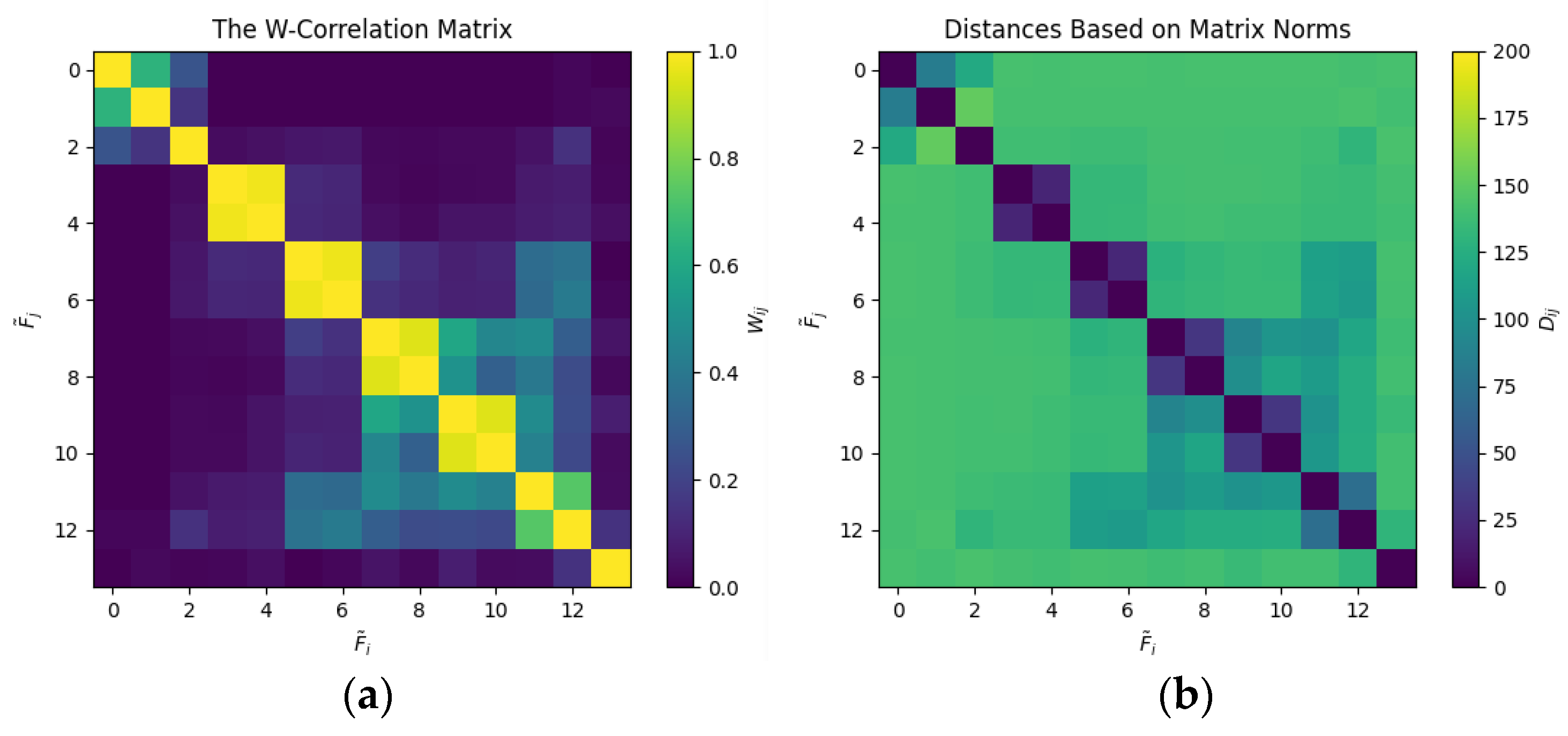
| Classification based on the w-correlation matrices of the principal components (Figure 8a) | Trend: {σ0, σ1, σ2} Harmonic: {σ3, σ4; σ5, σ6; σ7, σ8; σ9, σ10} Noise: {σ11–σ19} |
| Classification based on the correlation of the principal component matrices using the Frobenius norm (Figure 8b) | Trend: {σ0, σ1, σ2} Harmonic: {σ3, σ4; σ5, σ6; σ7, σ8; σ9, σ10} Noise: {σ11–σ19} |
| Proposed algorithm | Trend: {σ0, σ1, σ2} Harmonic: {σ3, σ4; σ5, σ6; σ7, σ8; σ9, σ10} Noise: {σ11–σ19} |
| Method | Hankelized Principal Components Matrices X1 | Hankelized Principal Components Matrices X2 (Figure A1) | Hankelized Principal Components Matrices X3 (Figure A2) | Hankelized Principal Components Matrices X4 (Figure A3) |
|---|---|---|---|---|
| Visual analysis of singular values | {σ0, σ1, σ2} {σ3, σ4; σ5, σ6; σ7, σ8; σ9, σ10} {σ11–σ19} | {σ0, σ1, σ2, σ3} {σ4, σ5} {σ6–σ19} | {σ6, σ7} {σ0, σ1; σ2, σ3; σ4, σ5; σ8, σ9; σ10, σ11} {σ12–σ19} | {σ4} {σ0, σ1; σ2, σ3; σ5, σ6} {σ7–σ19} |
| Classification based on the w-correlation matrices of the principal components | {σ0, σ1, σ2} {σ3, σ4; σ5, σ6; σ7, σ8; σ9, σ10} {σ11–σ19} | {σ0, σ1, σ2, σ3, σ6, σ7} {σ4, σ5; σ8, σ9} {σ10–σ19} | {σ6, σ7} {σ0, σ1; σ2, σ3; σ4, σ5; σ8, σ9} {σ10–σ19} | {σ4} {σ0, σ1; σ2, σ3; σ5, σ6} {σ7–σ19} |
| Classification based on the correlation of the principal component matrices using the Frobenius norm | {σ0, σ1, σ2} {σ3, σ4; σ5, σ6; σ7, σ8; σ9, σ10} {σ11–σ19} | {σ0, σ1, σ2, σ3, σ6, σ7} {σ4, σ5; σ8, σ9} {σ10–σ19} | {σ6, σ7} {σ0, σ1; σ2, σ3; σ4, σ5; σ8, σ9} {σ10–σ19} | {σ4} {σ0, σ1; σ2, σ3; σ5, σ6} {σ7–σ19} |
| Proposed algorithm | {σ0, σ1, σ2} {σ3, σ4; σ5, σ6; σ7, σ8; σ9, σ10} {σ11–σ19} | {σ0, σ1, σ2, σ3} {σ4, σ5} {σ6–σ19} | {σ6, σ7} {σ0, σ1; σ2, σ3; σ4, σ5; σ8, σ9; σ10, σ11} {σ12–σ19} | {σ4} {σ0, σ1; σ2, σ3; σ5, σ6} {σ7–σ19} |
Publisher’s Note: MDPI stays neutral with regard to jurisdictional claims in published maps and institutional affiliations. |
© 2022 by the authors. Licensee MDPI, Basel, Switzerland. This article is an open access article distributed under the terms and conditions of the Creative Commons Attribution (CC BY) license (https://creativecommons.org/licenses/by/4.0/).
Share and Cite
Bureneva, O.; Safyannikov, N.; Aleksanyan, Z. Singular Spectrum Analysis of Tremorograms for Human Neuromotor Reaction Estimation. Mathematics 2022, 10, 1794. https://doi.org/10.3390/math10111794
Bureneva O, Safyannikov N, Aleksanyan Z. Singular Spectrum Analysis of Tremorograms for Human Neuromotor Reaction Estimation. Mathematics. 2022; 10(11):1794. https://doi.org/10.3390/math10111794
Chicago/Turabian StyleBureneva, Olga, Nikolay Safyannikov, and Zoya Aleksanyan. 2022. "Singular Spectrum Analysis of Tremorograms for Human Neuromotor Reaction Estimation" Mathematics 10, no. 11: 1794. https://doi.org/10.3390/math10111794
APA StyleBureneva, O., Safyannikov, N., & Aleksanyan, Z. (2022). Singular Spectrum Analysis of Tremorograms for Human Neuromotor Reaction Estimation. Mathematics, 10(11), 1794. https://doi.org/10.3390/math10111794