Solute Transport Control at Channel Junctions Using Adjoint Sensitivity

Abstract

Water quality control and the control of contaminant spill in water in particular are becoming a primary need today. Gradient descent sensitivity methods based on the adjoint formulation have proved to be encouraging techniques in this context for river and channel flows. Taking into account that most channels and rivers include junctions with other branches, the objective of this study is to explore the adjoint technique on a channel network to reconstruct the upstream boundary condition of the convection-reaction equation. For this purpose, the one-dimensional shallow water equations and the transport equation for a reactive solute are considered. The control is formulated through the gradient-descent technique supplied with a first-order iterative process. Both the physical and the adjoint equations are supplied with suitable internal boundary conditions at the junction and are numerically solved using a finite volume upwind scheme. The results reveal that the adjoint technique is capable of reconstructing the inlet solute concentration boundary condition in an acceptable number of iterations for both steady state and transient configurations using a downstream measurement location. It was also observed that the reconstruction of the boundary condition tends to be less effective the further away the measurement station is from the target.

1. Introduction

Simulation tools based on hydrodynamic models combined with solute transport have become an essential tool to help decision makers [1], with efficiency and accuracy being both the fundamental keys of any mathematical model. Particularly, the geometry of the cross sections as well as the presence of junctions must be included into the model, having this last feature a greater impact on the physical and chemical properties of water. The numerical simulation of water flow at channel junctions has been addressed by several authors. In [2], it was concluded that it is possible to model the flow in a junction when the Froude numbers are low assuming the same water stage at the junction for every channel. Hsu et al. [3] derived an analytical approach through the junction over subcritical flows and uniform beds. The validation of their model was supported by three experimental tests with different junction angles, showing a good correlation between the numerical data and experimental values. The hydrodynamic details of flows at junctions have also been studied in [4,5,6,7,8] with experimental data and with field measurements. Likewise, the flow propagation in open-channel junctions was analyzed in [9], showing acceptable numerical results for supercritical transitions with small junction angles.

The influence of geometry in large-scale junctions was evaluated by [10]. It was concluded that there is a domain of the Kelvin–Helmholtz (KH) mode and the wake mode within the mixing interface, as the angle of the junction is altered. Based on the flow structure in the confluences, Constantinescu et al. [11] determined that the mixing interface can be either in the KH mode or in the wake mode. Both cases are dominated by quasi two-dimensional (2-D) eddies whose growth in the first case is boosted by the KH instability whereas, in the latter case, the mixing interface is populated by eddies with opposing senses of rotation. The influence of the mixing interface eddies and vortical characteristics on the mean velocity and turbulent kinetic energy patterns was also analyzed in [12]. Using the detached eddy simulation model, they were able to capture in detail the flow and turbulent structure in the confluence zone. This behavior was verified by a real data event at the confluence of the Kaskaskia River and Copper Slough. The morphological characteristics of the channel were also considered in [13,14]. In these studies, it was observed that sediment deposition is within and beyond the flow separation region, forming a large bank-attached bar.

On the other hand, the chemical change generated by the junction of two streams has been much more limited due to the requirements on the experimental data. Burguete et al. [15] demonstrated the innovative aspects for fertigation in furrows and level furrow systems with solute transport. This work was validated against experimental data and incorporated a computationally efficient approach of the internal boundary conditions to ensure the conservation of global mass. The behavior of the concentrations at junctions was also analyzed in [16]. Detailed analysis at the junction showed that the concentration distributions were controlled mainly by the shear layer and the two helical cells. The detailed study for dynamic phosphorus contamination was also considered in [17,18], showing and application for the Huiji and Ying rivers in eastern China. Additionally, it was demonstrated that there is an alteration of the flow and the mixing interface in junctions of two tributaries in natural rivers with large bed discordance due to the temperature differences in the two inflows [19]. Particularly, the mixing interface is proved to be very sensitive to inflow changes due to seasonal variations, which may cause significant differences in density [20].

The quality of the predictions supplied by numerical models is strongly related with the quality of the data used (initial conditions, boundary conditions or model parameters). This information is not always available for different reasons, and thus, retrieval techniques such as trial and error methods are necessary, sometimes resulting in tedious and not very intuitive processes especially when there is not enough modeling experience. To overcome this drawback, the gradient-descent method emerges as an alternative due to the use of the functional gradient where the minimum of the objective function is efficiently found. In this context, based on existing works [21,22,23,24,25,26], the adjoint method is considered to reconstruct a part or all of the necessary information in predictive simulation models. In particular, it is possible to efficiently reconstruct the boundary condition of a water quality model [27].

With this technique, the sensitivity of an objective function to the parameters of the system—initial, boundaries or decay coefficients—can be found by solving the adjoint equation backwards in time. This sensitivity is used in an iterative process, producing a sequence of improved solutions that ends up providing the desired values.

In this work, a one-dimensional (1D) hydrodynamic model combined with the advec-tion-reaction equation on a channel junction are used for the predictive simulation of the flow evolution and solute transport, respectively. The adjoint methodology is adopted to find a procedure to reconstruct the boundary condition of the transport equation using a measure of the error at a location downstream the junction. To meet this objective, the flow, the transport and the adjoint equations are solved using an explicit finite volume method. Particular attention is paid to the following aspects: (a) reconstruction of the inlet boundary condition of one or more solutes from downstream measurements after a junction; (b) validation of the numerical technique against steady state and unsteady scenarios of both flow and concentration; (c) characterization of the main strengths and limitations of the adjoint method; (d) test the reconstruction of the information, with different decay rates when more than one solute acts.

The rest of the paper is structured as follows: Section 2 presents the governing equations of the physical system together with the numerical method chosen to solve them. The adjoint formulation is provided in Section 3 and is also presented together with the numerical discretization used. In Section 4, the proposed model control is validated with some synthetic cases. The results of the model are presented in Section 5. Finally, the conclusions are presented for some test cases are discussed in Section 6.

2. Flow Equations and Numerical Model

The 1D Saint Venant equations are here considered to model the water flow [28] while the advection-reaction equation is used to model the solute transport with a first order decay process [29,30]. Diffusion–dispersion effects (particularly longitudinal dispersion) are important when modeling the behavior of solutes in rivers, mainly in accidental pollution problems [31,32]. However, for the sake of clarity, they have not been included in this work. The main reason for this is to simplify the development of this methodology without introducing another degree of freedom and extra uncertainty in the derivation of the equations and their resolution. Additionally, boundary conditions are needed for the whole set of the equations both at the inlet and outlet points and at the junctions. All these items are explained in the following paragraphs.

2.1. 1D Shallow Water Equations

The cross-sectional averaged 1D system of mass and momentum equations can be expressed as follows [33]:

$$\begin{array}{c}\hfill \begin{array}{cc}& \frac{\partial A}{\partial t}+\frac{\partial Q}{\partial x}=q_L\hfill \\ & \frac{\partial Q}{\partial t}+\frac{\partial }{\partial x}\left(\frac{Q^2}{A}+g{I}_1\right)=g[I_2+A(S_o-S_f)]\hfill \end{array}\end{array}$$

(1)

where $A\left[{\mathrm{L}}^2\right]$ is the wetted cross section area, $Q\left[{\mathrm{L}}^3{\mathrm{T}}^{-1}\right]$ is the discharge, $q_L\left[{\mathrm{L}}^2{\mathrm{T}}^{-1}\right]$ is the lateral inflow per unit width, $g\left[{\mathrm{LT}}^{-2}\right]$ is the acceleration due to gravity, $I_1\left[{\mathrm{L}}^3\right]$ represents the hydrostatic pressure force term, and $I_2\left[{\mathrm{L}}^2\right]$ accounts for the pressure forces due to channel width change. The remaining two terms $S_o\left[{\mathrm{LL}}^{-1}\right]$ and $S_f\left[{\mathrm{LL}}^{-1}\right]$ represent the bed slope and friction slope, the latter formulated with the semi-empirical Manning’s law:

$$\begin{array}{c}\hfill \begin{array}{c}\hfill S_o=-\frac{\partial z}{\partial x},S_f=\frac{n^2\left|Q\right|Q}{A^2{R}_h^{4/3}},\end{array}\end{array}$$

(2)

being $z\left[\mathrm{L}\right]$ the bed level, $R_h\left[\mathrm{L}\right]$ the hydraulic radius and $n\left[{\mathrm{TL}}^{-1/3}\right]$ the Manning’s roughness coefficient.

2.2. 1D Advection–Reaction Equation

The continuous change of concentration within the hydrodynamic system is generally affected by the advection and reaction processes. The formulation of this transport equation along every river or channel reach averaged in the cross section can be expressed as [34]:

$$\frac{\partial \left(A\varphi \right)}{\partial t}+\frac{\partial \left(Q\varphi \right)}{\partial x}=-AR,$$

(3)

where $\varphi \left[{\mathrm{ML}}^{-3}\right]$ is the cross sectional average concentration of the solute, and $R\left[{\mathrm{ML}}^{-3}{\mathrm{T}}^{-1}\right]$ is the first order rate or decay process:

$$R=\kappa \varphi ,$$

(4)

where $\kappa \left[{\mathrm{T}}^{-1}\right]$ is the reaction constant. As many transport equations as solutes must be considered together with the corresponding reaction terms in the case of more than one reactive solute in the system. This is accomplished simply by generalizing the concentration ${\varphi }_j$ and $R_j$ in (3) where the subscript j indicates the number of reactive solutes [35].

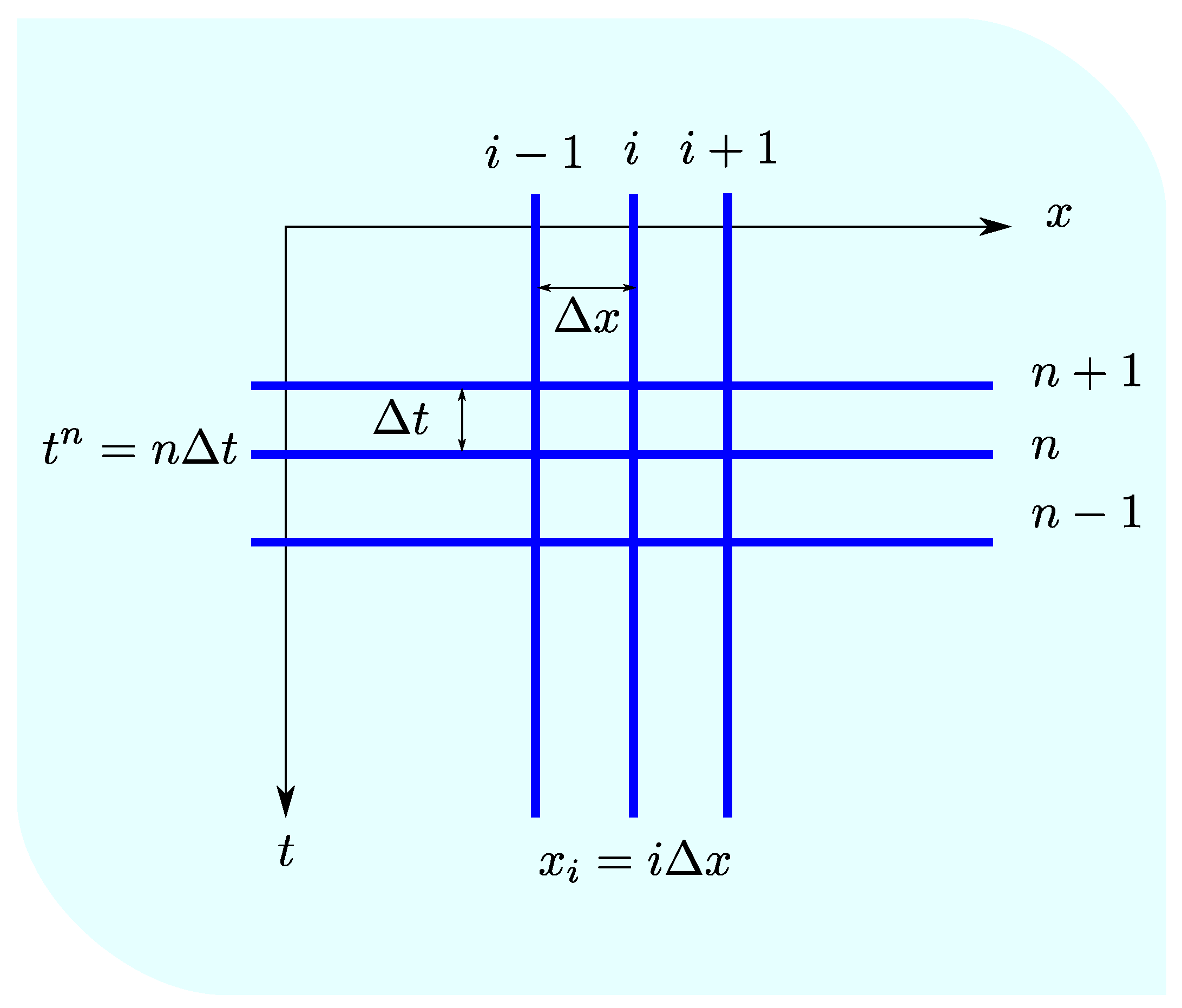
2.3. Numerical Model

The numerical solution of Equations (1) and (3) is achieved by applying an explicit upwind finite volume method based on Roe’s linearization. This scheme has been proved to be robust, well-balanced and efficient and has been verified in multiple scenarios: for the 1D and 2D the frameworks [36,37,38].

Following [15,38], the system (1) can be solved for each computational cell i of size $\Delta x$:

$$\begin{array}{c}\hfill \begin{array}{cc}\hfill {\mathbf{U}}_i^{n+1}=& {\mathbf{U}}_i^n-\frac{\Delta t}{\Delta x}{\left[{\left(\sum _m{\tilde{\lambda }}^{+}\tilde{\gamma }\tilde{\mathbf{e}}\right)}_{i-1/2}^m+{\left(\sum _m{\tilde{\lambda }}^{-}\tilde{\gamma }\tilde{\mathbf{e}}\right)}_{i+1/2}^m\right]}^n,\hfill \end{array}\end{array}$$

(5)

where $\mathbf{U}=(A,Q)$, n is the discrete time level, and $\tilde{\lambda }$ and $\tilde{\mathbf{e}}$ are the eigenvalues and eigenvectors, respectively; $\tilde{\gamma }$ is the linearized term that contains the fluxes and source strengths; m is the eigenvalues counter, and $\Delta t$ is the time step size. This Expression (5) is solved for the interior points in each of the channels considered in the system.

The complete discretization of the transport equation follows [39]:

$$\begin{array}{c}\hfill {\left(A\varphi \right)}_i^{n+1}={\left(A\varphi \right)}_i^n-\frac{\Delta t}{\Delta x}{\left[{\left(q\varphi \right)}_{i+1/2}^{\downarrow }-{\left(q\varphi \right)}_{i-1/2}^{\downarrow }\right]}^n+\Delta t{\left(AR\right)}_i^n,\end{array}$$

(6)

where the variables $q^{\downarrow }$ and ${\varphi }^{\downarrow }$ are defined in order to decouple conservatively this equation from the hydrodynamic system. This formulation ensures solute positivity and a non-oscillatory solution in both space and time [35]. The scheme in (6) is used to solve for each solute at all the interior points of each channel.

2.4. Junction Boundary Conditions

Appropriate boundary conditions are needed to solve the system of flow and solute equations formed by (1) and (3). The number of boundary conditions at the inlet, outlet and junction points depends on the flow regime [2]. For the sake of simplification, this work only considers sub-critical cases. Regarding the flow equations, it is enough to impose one boundary condition upstream and downstream. Generally, a discharge hydrograph $Q\left(t\right)$ is imposed upstream while a gauging curve or a water surface level is set downstream. As for the solute, only an upstream boundary condition is required.

When considering junctions such as the one represented in Figure 1, internal boundary conditions are needed. In the present work, uniform water surface level together with discharge continuity at the junction is assumed [40]:

$$\begin{array}{cc}\hfill & {(h+z)}_{imax,1}={(h+z)}_{0,2}={(h+z)}_{imax,3},\hfill \\ \hfill & Q_{0,2}=Q_{imax,1}\pm Q_{imax,3},\hfill \end{array}$$

(7)

where the number of cells goes from 0 to $imax$ in each channel. As for the internal condition of the solute, a mass balance at the junction is formulated as in [15]:

$${\left(Q\varphi \right)}_{0,2}={\left(Q\varphi \right)}_{imax,1}\pm {\left(Q\varphi \right)}_{imax,3}.$$

(8)

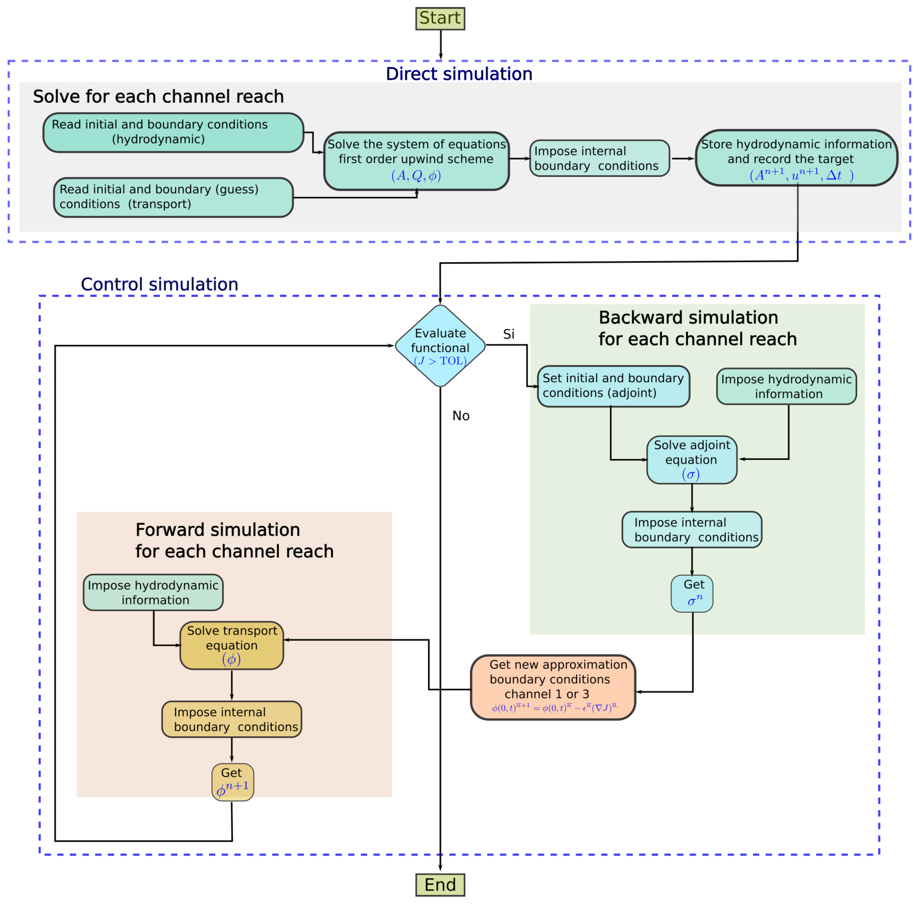
3. Adjoint Equations and Gradient Descent Method

3.1. Solute Transport Adjoint Equation

This study focuses on identifying the sensitivity of the objective function to the inlet boundary condition of one or more solutes on a network of channels with junctions. For this purpose, an objective function is defined in order to measure the error between the values of the concentration predicted by the numerical simulation and those measured at a certain location ($x_M$):

$$J\left(p\right)=\frac{1}{2}{\int }_0^T{\int }_0^L\left[{\delta }_D(x-x_M){(\varphi \left(p\right)-\widehat{\varphi })}^2\right]dxdt,$$

(9)

where ${\delta }_D\left(\right)$ is the Dirac-delta function, $\varphi \left(p\right)$ is the computed concentration based on a parameter p which the functional depends on, $\widehat{\varphi }$ is the target at location $x_M$, $T\left[\mathrm{T}\right]$ is the total simulation time, and $L\left[\mathrm{L}\right]$ refers to the length of the computational domain.

The method to derive the adjoint equation from the configuration shown in Figure 1, where the measurement point is assumed in channel 2, is summarized in the following steps: (1) The transport Equation (3) is multiplied by an adjoint variable ($\sigma \left[{\mathrm{MTL}}^{-5}\right]$) and integrated in space and time for each channel k:

$$\begin{array}{c}\hfill \begin{array}{cc}& I={\int }_0^T{\int }_{x_{0,1}}^{x_{imax,1}}{\sigma }_1{\left[\frac{\partial \left(A\varphi \right)}{\partial t}+\frac{\partial \left(Q\varphi \right)}{\partial x}+AR\right]}_{1}dxdt\hfill \\ & +{\int }_0^T{\int }_{x_{0,2}}^{x_{imax,2}}{\sigma }_2{\left[\frac{\partial \left(A\varphi \right)}{\partial t}+\frac{\partial \left(Q\varphi \right)}{\partial x}+AR\right]}_{2}dxdt\hfill \\ & +{\int }_0^T{\int }_{x_{0,3}}^{x_{imax,3}}{\sigma }_3{\left[\frac{\partial \left(A\varphi \right)}{\partial t}+\frac{\partial \left(Q\varphi \right)}{\partial x}+AR\right]}_{3}dxdt=0.\hfill \end{array}\end{array}$$

(10)

(2) Integrating (10) by parts, the partial derivatives are passed over to the adjoint variable:

$$\begin{array}{c}\hfill \begin{array}{cc}\hfill I& ={\int }_0^T{\int }_{x_{0,1}}^{x_{imax,1}}{\left[-\left(A\varphi \right)\frac{\partial \sigma }{\partial t}-\left(Q\varphi \right)\frac{\partial \sigma }{\partial x}+A\sigma R\right]}_{1}dxdt\hfill \\ & +{\int }_0^T\sigma Q\varphi {|}_{x_{0,1}}^{x_{imax,1}}dt+{\int }_{x_{0,1}}^{x_{imax,1}}\sigma A\varphi {|}_0^{T}dx\hfill \\ & +{\int }_0^T{\int }_{x_{0,2}}^{x_{imax,2}}{\left[-\left(A\varphi \right)\frac{\partial \sigma }{\partial t}-\left(Q\varphi \right)\frac{\partial \sigma }{\partial x}+A\sigma R\right]}_{2}dxdt\hfill \\ & +{\int }_0^T\sigma Q\varphi {|}_{x_{0,2}}^{x_{imax,2}}dt+{\int }_{x_{0,2}}^{x_{imax,2}}\sigma A\varphi {|}_0^{T}dx\hfill \\ & +{\int }_0^T{\int }_{x_{0,3}}^{x_{imax,3}}{\left[-\left(A\varphi \right)\frac{\partial \sigma }{\partial t}-\left(Q\varphi \right)\frac{\partial \sigma }{\partial x}+A\sigma R\right]}_{3}dxdt\hfill \\ & +{\int }_0^T\sigma Q\varphi {|}_{x_{0,3}}^{x_{imax,3}}dt+{\int }_{x_{0,3}}^{x_{imax,3}}\sigma A\varphi {|}_0^{T}dx=0.\hfill \end{array}\end{array}$$

(11)

(3) As $I=0$, we can redefine (9) as $J=J+I$ and taking the first variation of the functional with respect to $\varphi$ leads to

$$\begin{array}{c}\hfill \begin{array}{cc}\hfill \delta J& ={\int }_0^T{\int }_{x_{0,1}}^{x_{imax,1}}{\left[-\left(A\delta \varphi \right)\frac{\partial \sigma }{\partial t}-\left(Q\delta \varphi \right)\frac{\partial \sigma }{\partial x}+A\frac{\partial R}{\partial \varphi }\delta \varphi \right]}_{1}dxdt\hfill \\ & +{\int }_0^T\sigma Q\delta \varphi {|}_{x_{0,1}}^{x_{imax,1}}dt{\int }_{x_{0,1}}^{x_{imax,1}}\sigma A\delta \varphi {|}_0^{T}dx\hfill \\ & +{\int }_0^T{\int }_{x_{0,2}}^{x_{imax,2}}{\delta }_D(x-x_M)\frac{\partial \xi }{\partial \varphi }\delta \varphi dxdt+\hfill \\ & +{\int }_0^T{\int }_{x_{0,2}}^{x_{imax,2}}{\left[-\left(A\delta \varphi \right)\frac{\partial \sigma }{\partial t}-\left(Q\delta \varphi \right)\frac{\partial \sigma }{\partial x}+A\frac{\partial R}{\partial \varphi }\delta \varphi \right]}_{2}dxdt\hfill \\ & +{\int }_0^T\sigma Q\delta \varphi {|}_{x_{0,2}}^{x_{imax,2}}dt+{\int }_{x_{0,2}}^{x_{imax,2}}\sigma A\delta \varphi {|}_0^{T}dx\hfill \\ & +{\int }_0^T{\int }_{x_{0,3}}^{x_{imax,3}}{\left[-\left(A\delta \varphi \right)\frac{\partial \sigma }{\partial t}-\left(Q\delta \varphi \right)\frac{\partial \sigma }{\partial x}+A\frac{\partial R}{\partial \varphi }\delta \varphi \right]}_{3}dxdt\hfill \\ & +{\int }_0^T\sigma Q\delta \varphi {|}_{x_{0,3}}^{x_{imax,3}}dt+{\int }_{x_{0,3}}^{x_{imax,3}}\sigma A\delta \varphi {|}_0^{T}dx,\hfill \end{array}\end{array}$$

(12)

with

$$\xi =\frac{1}{2}{(\varphi \left(p\right)-\widehat{\varphi })}^2.$$

(13)

(4) With the aim of finding the sensitivities of the objective function with respect to the upstream boundary condition of the first channel, certain restrictions are applied:

$$\begin{array}{c}\hfill \begin{array}{cc}& \sigma (x_k,T)=0,k=1,\dots ,3,\hfill \\ & \delta \varphi (x_k,0)=0,k=1,\dots ,3,\hfill \\ & \delta \varphi (x_{imax,2},t)=\delta \varphi (x_{0,3},t)=0.\hfill \end{array}\end{array}$$

(14)

(5) The adjoint equations are formulated at every channel reach k:

$$\begin{array}{c}\hfill {\left[-A\frac{\partial \sigma }{\partial t}-Q\frac{\partial \sigma }{\partial x}+\frac{\partial \xi }{\partial \varphi }-A\sigma \frac{\partial R}{\partial \varphi }\right]}_k=0.k=1,\dots ,3\end{array}$$

(15)

The adjoint advection–reaction equations are in charge of transporting the error registered at the measurement station ($x_M$) to the reconstruction point, which is in this case the inlet boundary of channel 1.

(6) Now, applying the constraints of Equations (14) and (15) on Expression (12) leads to

$$\begin{array}{c}\hfill \begin{array}{cc}& \delta J={\int }_0^T\left[{\left(\sigma Q\delta \varphi \right)}_{x_{imax,1}}-{\left(\sigma Q\delta \varphi \right)}_{x_{0,1}}-{\left(\sigma Q\delta \varphi \right)}_{x_{0,2}}+{\left(\sigma Q\delta \varphi \right)}_{x_{imax3}}\right]dt.\hfill \end{array}\end{array}$$

(16)

(7) Like the flow and transport equations, the adjoint equations also require an internal boundary condition at the junction.

$${\left(\sigma Q\delta \varphi \right)}_{x_{imax1}}-{\left(\sigma Q\delta \varphi \right)}_{x_{0,2}}+{\left(\sigma Q\delta \varphi \right)}_{x_{imax,3}}=0.$$

(17)

(8) Accordingly, the sensitivity of the objective function to the boundary condition of channel 1 is

$$\begin{array}{c}\hfill \nabla J=\frac{\delta J}{\delta \varphi }{|}_{{(0,t)}_1}=-\left(\sigma Q\right){(0,t)}_1.\end{array}$$

(18)

Therefore, the regulation can be applied by means of the perturbation in the value of the boundary condition $\varphi (0,t)$ using the discrete version of (18) at every time $t^n$. This development is part of an iterative process that is detailed later.

Note that the technique described above is analogous to reconstruct the boundary condition at channel 3.

3.2. Numerical Model and Gradient Descent Method

The adjoint equations (15) can be discretized (see Figure 2) following the same procedure used in (6). Therefore, the expression that updates the adjoint variables at cell i for time $t^n$ is [27]:

$${\sigma }_i^n={\sigma }_i^{n+1}+\frac{\Delta t}{\Delta x}\left[{\left(u^{-}\delta \sigma \right)}_{i-1/2}^{n+1}+{\left(u^{+}\delta \sigma \right)}_{i+1/2}^{n+1}\right]+\Delta t{\left(\sigma R\right)}_i+\Delta t{\left(\frac{\partial \xi }{\partial \varphi }\frac{1}{A}\right)}_i$$

(19)

where $u=Q/A$ is the cross sectional average flow velocity. It is worth highlighting that finding the solution of the adjoint variable $\sigma$ for each channel requires to solve the system backwards in time, that is, updating the time as $t^n=t^{n+1}-\Delta t$. Note that the upwind contributions (positive or negative superindex in the flow velocity) are opposite to those on the transport equation. As seen, the solution of Equation (19) also requires some information such as the time step $\Delta t$, the flow velocity $u_i^n$ and the wetted area $A_i^n$ at every time level $t^n$. For this purpose, all the information regarding the hydrodynamic part is saved at each time step and at each computational cell in a previous first forward simulation. Due to the explicit character of the scheme, the time step size is restricted by stability reasons in order to fulfill the CFL condition [35,41].

To obtain the best reconstructed values for the boundary condition, the gradient-descent method is used. The form of the iterative algorithm is described as follows:

$$\varphi {(0,t)}^{\overline{n}+1}=\varphi {(0,t)}^{\overline{n}}-{ϵ}^{\overline{n}}{(\nabla J)}^{\overline{n}},$$

(20)

where $\overline{n}$ indicates the level of the iteration, $ϵ$ is the step length, and $\nabla J$ is the gradient of J. Accordingly, as long as all the hydrodynamic information is available, only of the adjoint equation (backwards) and the transport equation (forward) are necessary to converge to the minimum of the function with a certain tolerance.

The step length $ϵ$ is considered a constant value and is obtained through trial and error. Regarding the target, the location of the measuring station $x_M$ does not follow a defined rule; however, according to a previous work [42], it is known that this location could be crucial when reconstructing the information at a given point.

Figure 3 illustrates the flowchart followed to reconstruct the information of the solute boundary condition. This process is summarized in two fundamental stages: the so-called flow simulation and the control simulation. In the flow simulation, the flow equations are solved using (5) with the known initial and boundary conditions, while the transport equation is computed with an estimated boundary condition (initial guess, generally 0) using (6). All the hydrodynamic information necessary for the next stage is stored during this process.

For the control simulation, two main parts are considered: the forward simulation and the backward simulation. This process is repeated until the functional is below a tolerance. The backward simulation calculates the value of the adjoint variable using (19) and the available velocity field and time step size at each time level and at each computational cell. The upstream boundary condition, i.e., the new value of the concentration at every time level, is obtained through the gradient method using (20).

4. Test Cases

The robustness and accuracy of the proposed technique is verified with some synthetic cases. In all of them, a first simulation is performed using a known upstream boundary condition in order to store time series of concentration values at the measurement point to be used as the target. These values are then used as the “experimental data” for the adjoint technique in order to evaluate the ability of the proposed method to reconstruct the upstream solute boundary condition.

The optimization process starts by solving the transport equation with an initial guess inlet solute boundary condition $\varphi {(0,t)}_1=0\mathrm{g}/{\mathrm{m}}^3$. The adjoint equation is then solved backwards to obtain the sensitivity for the optimization algorithm. The process is repeated until the functional value is below a tolerance level. This procedure is applied in all cases presented.

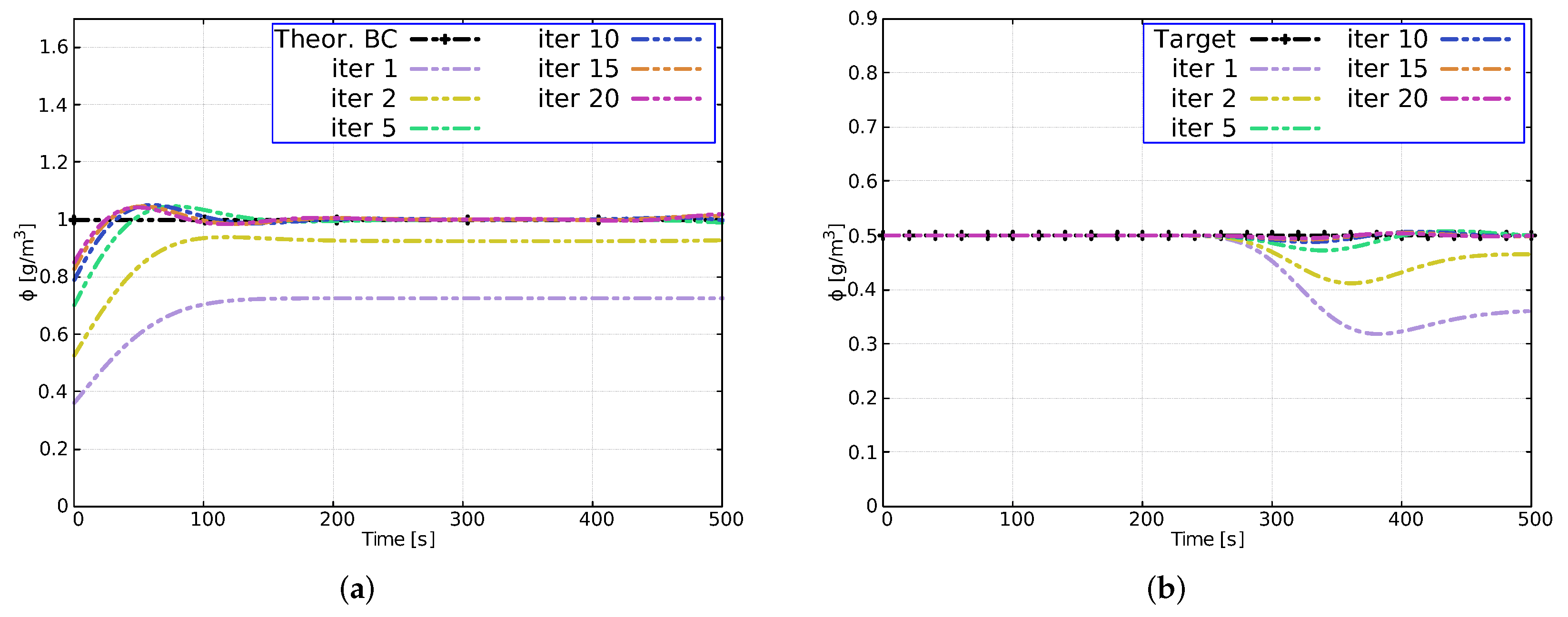
4.1. Cases 1 and 2: Steady State of Both Flow and Concentration

In this scenario, we consider a 90° junction of three 10 m wide rectangular flat and frictionless channels of lengths $L_1$, $L_2$ and $L_3$ and widths $B_1$, $B_2$ and $B_3$ as shown in Figure 4. The initial conditions are

$$\begin{array}{c}\hfill Q{(x,0)}_1=1{\mathrm{m}}^3/\mathrm{s}\varphi {(\mathrm{x},0)}_1=1\mathrm{g}/{\mathrm{m}}^3\mathrm{x}\in [0,{\mathrm{L}}_1]\\ \hfill Q{(x,0)}_2=2{\mathrm{m}}^3/\mathrm{s}\varphi {(\mathrm{x},0)}_2=0.5\mathrm{g}/{\mathrm{m}}^3\mathrm{x}\in [0,{\mathrm{L}}_2]\\ \hfill Q{(x,0)}_3=1{\mathrm{m}}^3/\mathrm{s}\varphi {(\mathrm{x},0)}_3=0\mathrm{g}/{\mathrm{m}}^3\mathrm{x}\in [0,{\mathrm{L}}_3]\end{array}$$

The inlet flow boundary condition is defined by the following values: $Q{(0,t)}_1=Q{(0,t)}_3=1$${\mathrm{m}}^3/\mathrm{s}$ for both channel 1 and channel 3 for $t\in [0,T]$. The solute inlet boundary condition for channel 3 is $\varphi {(x,0)}_3=0\mathrm{g}/{\mathrm{m}}^3$ for $x\in [0,L_3]$. The inlet boundary condition for the solute of the first channel to be reconstructed by means of the control is $\varphi {(0,t)}_1=1$$\mathrm{g}/{\mathrm{m}}^3$ for $t\in [0,T]$. For this case, the reaction constant $\kappa =0$.

The measurement station is located in channel 2 at $x_M=25.5\mathrm{m}$ (see Figure 4). As previously mentioned, these values are obtained through a first simulation with all the known parameters.

The time evolution of the solute concentration both at the inlet of channel 1 and at the target location in channel 2 obtained with CFL = 1, $\Delta x=1$ m and $ϵ=7$ are shown in Figure 5. The numerical solution with the proposed scheme is plotted for iterations 1, 2, 5, 10, 15 and 20 (colored lines) for both the boundary conditions (a) and the target (b). The numerical solution of the last iteration converges to the theoretical solution (black line) with an acceptable accuracy. Small differences show up at the beginning of the simulation ($t\in [0,150\mathrm{s}]$) for the boundary reconstruction. This behavior has already been reported and analyzed in the literature [27] and is attributed to the numerical diffusion. The target is however successfully achieved at iteration 20.

This test case has been repeated to evaluate the influence of the mesh size using the following number of cells (MNC): 100, 200 and 400. The results of both the reconstruction of the boundary condition in the last iteration and the evolution of the objective functional are plotted in Figure 6. Particularly, Figure 6a shows the variations that occur at the beginning of the simulation. They can be attributed to the numerical diffusion as well that tends to decrease as the mesh number of cells (MNC) increases.

The results of the objective function also show the same trend, i.e., its value decreases as the number of cells increases. Furthermore, it is evident that the functional does not decrease in the same way for the range of iterations, especially in the first 20 iterations. For example, for a fixed $J=1.0\times {10}^{-4}$, the number of iterations is different: ten iteration for MNC = 400, three iterations for MNC = 100. This trend changes after 20 iterations.

In the context of Case 1, new cases are considered (Case 2), to test the influence of the inlet discharge of channel. For this purpose, three scenarios were carried out. The initial conditions (I.C.) and boundary conditions (B.C.) of the flow of the three scenarios are displayed in

Table 1. Initial and inlet boundary conditions to evaluate the reconstruction of the inlet boundary condition of the solute at channel 3.

Case	I.C. $\mathit{Q}(\mathit{x},0){\mathbf{m}}^3/\mathbf{s}$			B.C. $\mathit{Q}(0,\mathit{t}){\mathbf{m}}^3/\mathbf{s}$
	Channel 1	Channel 2	Channel 3	Channel 1	Channel 3
Case 2.1	1	1.5	0.5	1	0.5
Case 2.2	1	2	1	1	1
Case 2.3	1	3	2	1	2

.

The initial condition of the solute for the three channels and for the three proposed cases is $\varphi (x,0)=1\mathrm{g}/{\mathrm{m}}^3$, and the boundary condition is determined by the following expression:

$$\varphi {(0,t)}_1=\left\{\begin{array}{c}10\le t\le 100\mathrm{s}\hfill \\ 0t\ge 100\mathrm{s}\hfill \end{array}\right.\varphi {(0,t)}_3=\left\{\begin{array}{c}10\le t\le 2000\mathrm{s}\hfill \\ 0t\ge 2000\mathrm{s}\hfill \end{array}\right.$$

The results show that the value of the functional tends to decrease the higher the inlet flow is. The discussion and the Root Mean Square Error (RMSE) of this set of test cases is presented later.

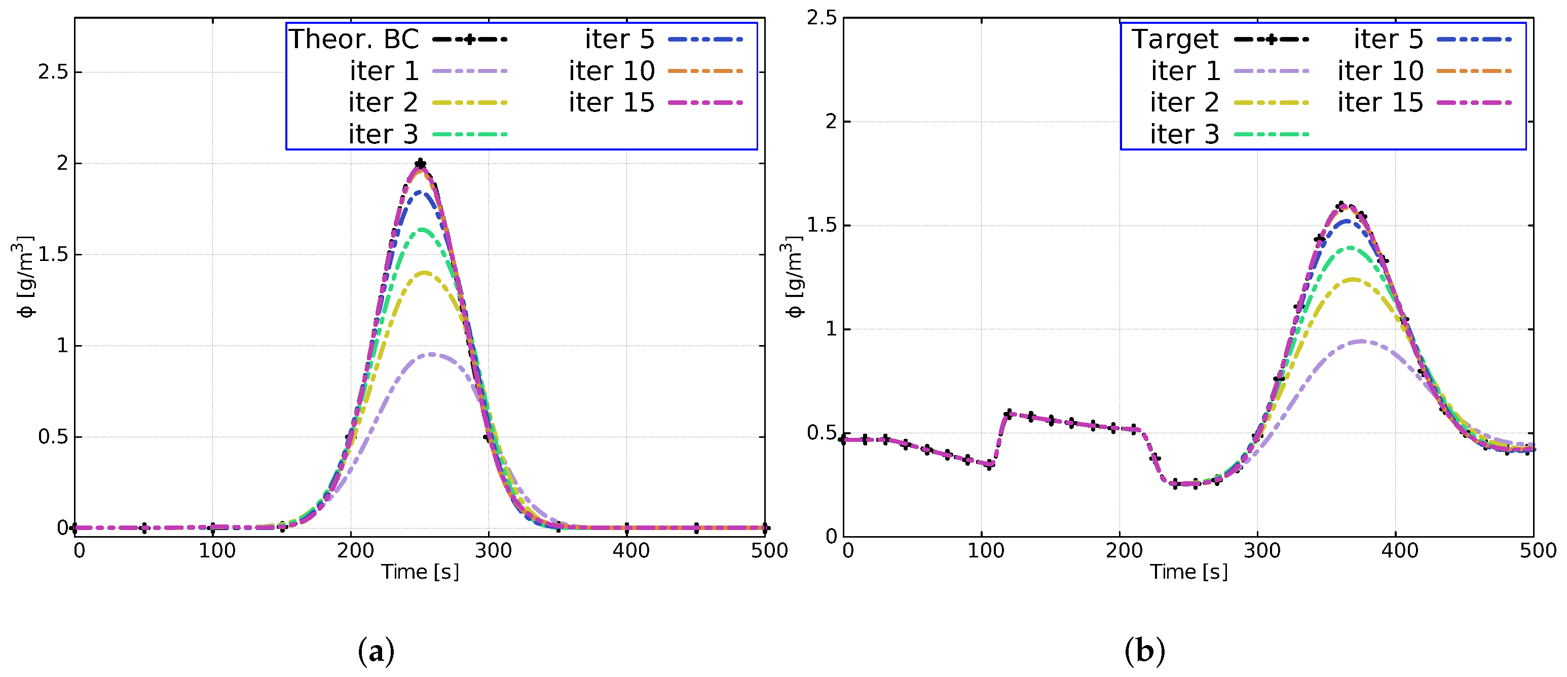
4.2. Case 3: Unsteady Flow with Gaussian Pulse for Both Flow and Concentration

This test case considers the same configuration displayed in Figure 4. The following initial conditions for both flow and solute are imposed:

$$\begin{array}{cc}\hfill & Q{(x,0)}_1=1.14{\mathrm{m}}^3/\mathrm{s}\varphi {(x,0)}_1=0\mathrm{g}/{\mathrm{m}}^3\mathrm{x}\in [0,{\mathrm{L}}_1]\hfill \\ \hfill & Q{(x,0)}_2=2.14{\mathrm{m}}^3/\mathrm{s}\varphi {(x,0)}_2=0.46\mathrm{g}/{\mathrm{m}}^3\mathrm{x}\in [0,{\mathrm{L}}_2]\hfill \\ \hfill & Q{(x,0)}_3=1{\mathrm{m}}^3/\mathrm{s}\varphi {(x,0)}_3=1\mathrm{g}/{\mathrm{m}}^3\mathrm{x}\in [0,{\mathrm{L}}_3]\hfill \end{array}$$

The hydrodynamic inlet boundary condition for channel 1 is defined with a Gaussian function expressed as

$$Q{(0,t)}_1=a{e}^{-\frac{{(t-b)}^2}{2c^2}}a=3,b=250,c=180t\in [0,T]$$

(21)

The solute boundary condition $\varphi {(0,t)}_1$ used to generate the target to be reconstructed by the adjoint method follows:

$$\varphi {(0,t)}_1=a{e}^{-\frac{{(t-b)}^2}{2c^2}}.a=2,b=250,c=30t\in [0,T]$$

(22)

On the other hand, the inlet boundary conditions at channel 3 are defined as

$$Q{(0,t)}_3=\left\{\begin{array}{c}1{\mathrm{m}}^3/\mathrm{s}t\in [0,100\mathrm{s}]\hfill \\ 3{\mathrm{m}}^3/\mathrm{s}t\in [100\mathrm{s},200\mathrm{s}]\hfill \\ 1{\mathrm{m}}^3/\mathrm{s}t\in [200\mathrm{s},500\mathrm{s}]\hfill \end{array}\right.\varphi {(0,t)}_3=1\mathrm{g}/{\mathrm{m}}^{3}t\in [0,T]$$

(23)

No reaction or decay processes are considered ($\kappa =0$). The downstream measurement station is located in channel 2 at $x_M=5.5$ m. As for the optimization method, $ϵ=8$. The numerical results are plotted in Figure 7. The method efficiently reconstructs the signals regardless of their distributions. Particularly, the shape of the target (see Figure 7b) containing a plateau and the Gaussian pulse coming from the input signals from channels 1 and 3 are satisfactory achieved. With only 15 iterations, it is possible to reconstruct the boundary condition at channel 1 and achieve a great level of accuracy at the target (channel 2) without any non-physical concentrations or oscillations.

4.3. Case 4: Analysis of the Influence of the Measurement Station, Geometry and the Type of Reconstruction

The purpose of the next set of cases is to observe the influence of the location of the measurement station and the geometry of the case (length, slope) in the performance of the adjoint technique for the reconstruction of the upstream solute boundary condition of either channel 1 or channel 3. The configuration of the channel system is similar to that shown in Figure 4. Initial conditions for these scenarios are

$$\begin{array}{cc}\hfill & Q{(x,0)}_1=1{\mathrm{m}}^3/\mathrm{s}\varphi {(x,0)}_1=0\mathrm{g}/{\mathrm{m}}^3\mathrm{x}\in [0,{\mathrm{L}}_1]\hfill \\ \hfill & Q{(x,0)}_2=2{\mathrm{m}}^3/\mathrm{s}\varphi {(x,0)}_2=0\mathrm{g}/{\mathrm{m}}^3\mathrm{x}\in [0,{\mathrm{L}}_2]\hfill \\ \hfill & Q{(x,0)}_3=1{\mathrm{m}}^3/\mathrm{s}\varphi {(x,0)}_3=0\mathrm{g}/{\mathrm{m}}^3\mathrm{x}\in [0,{\mathrm{L}}_3]\hfill \end{array}$$

The boundary conditions for all the cases presented are

$$Q{(0,t)}_1=\left\{\begin{array}{c}1t\in [0,100\mathrm{s}]\hfill \\ 2t\in [100,1100\mathrm{s}]\hfill \\ 1t\ge 1100\mathrm{s}\hfill \end{array}\right.\varphi {(0,t)}_1=\left\{\begin{array}{c}0t\in [0,100\mathrm{s}]\hfill \\ 2t\in [100,1100\mathrm{s}]\hfill \\ 0t\ge 1100\mathrm{s}\hfill \end{array}\right.$$

$$Q{(0,t)}_3=\left\{\begin{array}{c}0.5t\in [0,100\mathrm{s}]\hfill \\ 1t\in [100,1100\mathrm{s}]\hfill \\ 0.5t\ge 1100\mathrm{s}\hfill \end{array}\right.\varphi {(0,t)}_3=\left\{\begin{array}{c}0t\in [0,100\mathrm{s}]\hfill \\ 1t\in [100,1100\mathrm{s}]\hfill \\ 0t\ge 1100\mathrm{s}\hfill \end{array}\right.$$

The roughness coefficient is 0.035 ${\mathrm{sm}}^{-1/3}$, and $\Delta x=5$ m. This analysis is carried out by changing the length, slope and target location as shown in

Table 2. Case 4. Location of the target measuring station (channel 2) and geometric properties.

Channel Recons.	Case	${\mathit{L}}_1$ (m)	${\mathit{L}}_2$ (m)	${\mathit{L}}_3$ (m)	${\left({\mathit{S}}_{\mathit{o}}\right)}_{1-3}$	${\mathit{x}}_{\mathit{M}}$ (m)
channel 1	Case 3.1	1000	1000	1000	1%	100
	Case 3.2	1000	1000	1000	1%	500
	Case 3.3	1000	1000	1000	1%	900
	Case 3.4	500	1000	1000	1%	100
	Case 3.5	1000	1000	1000	1%	100
	Case 3.6	1500	1000	1000	1%	100
	Case 3.7	1000	1000	1000	0.5%	100
	Case 3.8	1000	1000	1000	1%	100
	Case 3.9	1000	1000	1000	1.5%	100
channel 3	Case 3.10	1000	1000	500	1%	100
	Case 3.11	1000	1000	1000	1%	100
	Case 3.12	1000	1000	1500	1%	100

. The results with $ϵ=1$, CFL = 1 and number of total iterations equal to 100 are plotted in Figure 8. According to the location of the measurement station (Figure 2a), the study shows that the further it is from the reconstruction point, the bigger that value of the functional is. Regarding the length, the functional adopts different forms according to the reconstruction, and when the reconstruction is on channel 1 (see Figure 2b), there are small differences between the functional. However, when the information of channel 3 is reconstructed (Figure 2d), there are large variations, especially when the length of channel 3 is 1500 m. On the other hand, when the slope is 2%, the value of the functional decreases considerably with respect to the 1% slope (see Figure 2c).

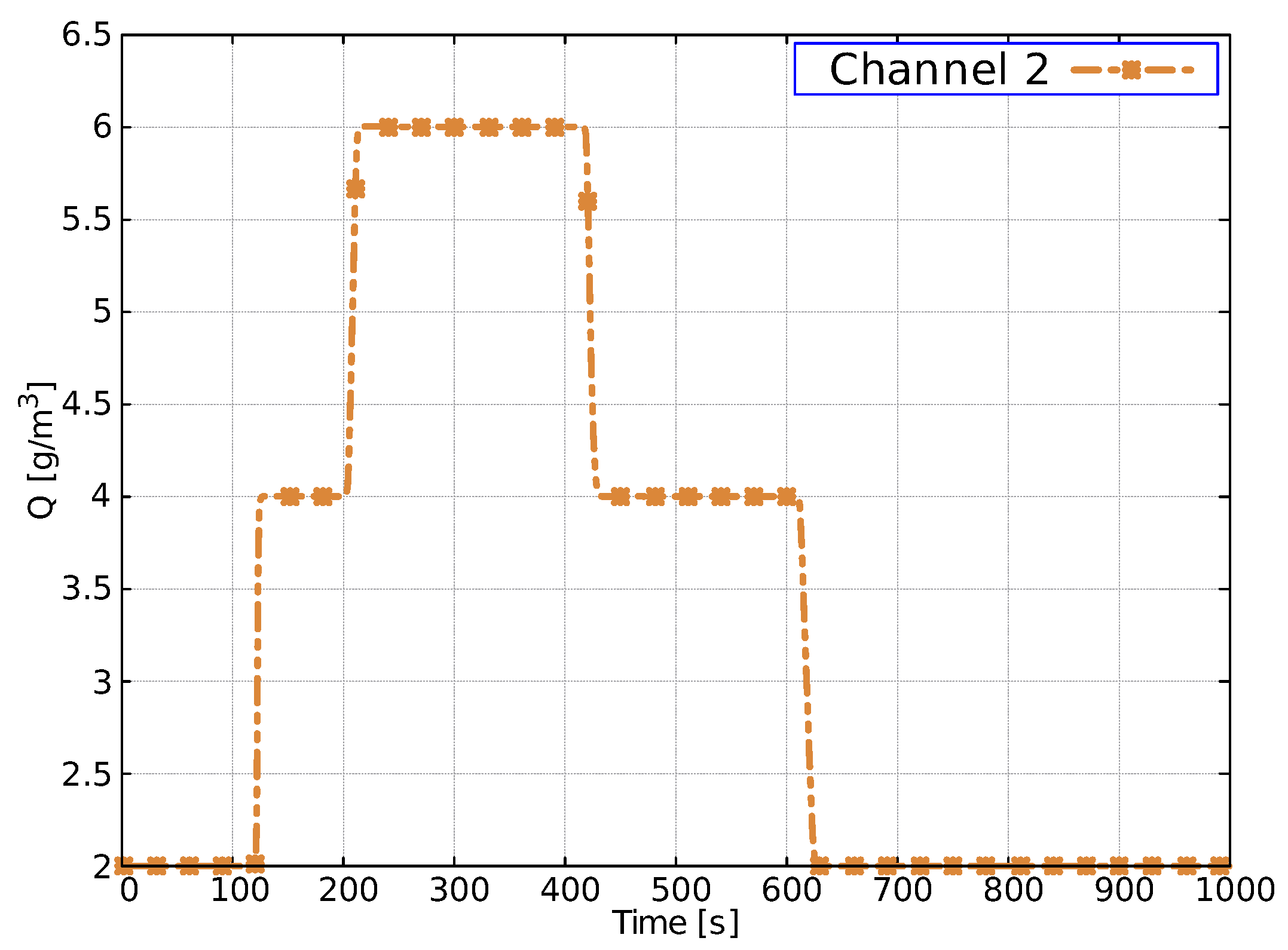
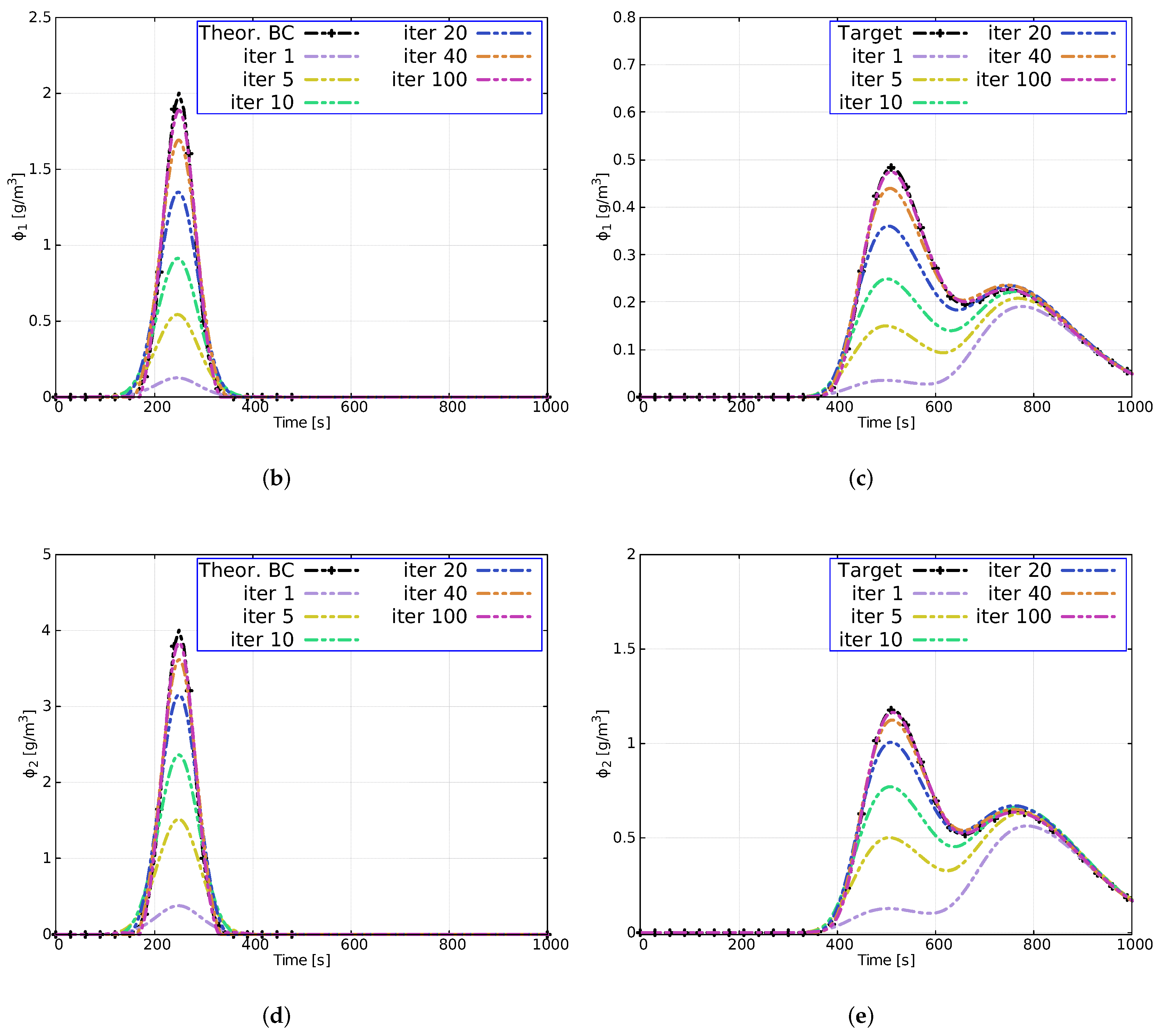
4.4. Case 5: Unsteady Flow with Step Pulse for Both Flow and Concentration with Reaction

The purpose of this case is to observe the behavior of the reconstruction of the channel 1 upstream boundary condition given by a solute step pulse on the same configuration of Case 1 in presence of reaction. The initial conditions are set according to

$$\begin{array}{c}\hfill Q{(x,0)}_1=1{\mathrm{m}}^3/\mathrm{s}\mathrm{x}\in [0,{\mathrm{L}}_1]\\ \hfill Q{(x,0)}_2=2{\mathrm{m}}^3/\mathrm{s}\mathrm{x}\in [0,{\mathrm{L}}_2]\\ \hfill Q{(x,0)}_3=1{\mathrm{m}}^3/\mathrm{s}\mathrm{x}\in [0,{\mathrm{L}}_3]\\ \hfill \varphi {(x,0)}_1=\varphi {(x,0)}_2=\varphi {(x,0)}_3=1\mathrm{g}/{\mathrm{m}}^3\mathrm{x}\in [0,{\mathrm{L}}_{\mathrm{k}}]\end{array}$$

(24)

and the boundary conditions are

$$Q{(0,t)}_1=\left\{\begin{array}{c}1{\mathrm{m}}^3/\mathrm{s}t\in [0,100\mathrm{s}]\hfill \\ 3{\mathrm{m}}^3/\mathrm{s}t\in [100\mathrm{s},400\mathrm{s}]\hfill \\ 1{\mathrm{m}}^3/\mathrm{s}t\in [400\mathrm{s},1000\mathrm{s}]\hfill \end{array}\right.\varphi {(0,t)}_1=\left\{\begin{array}{c}1\mathrm{g}/{\mathrm{m}}^{3}t\in [0,100\mathrm{s}]\hfill \\ 3\mathrm{g}/{\mathrm{m}}^{3}t\in [100\mathrm{s},400\mathrm{s}]\hfill \\ 1\mathrm{g}/{\mathrm{m}}^{3}t\in [400\mathrm{s},1000\mathrm{s}]\hfill \end{array}\right.$$

$$Q{(0,t)}_3=\left\{\begin{array}{c}1{\mathrm{m}}^3/\mathrm{s}t\in [0,200\mathrm{s}]\hfill \\ 3{\mathrm{m}}^3/\mathrm{s}t\in [200\mathrm{s},600\mathrm{s}]\hfill \\ 1{\mathrm{m}}^3/\mathrm{s}t\in [600\mathrm{s},1000\mathrm{s}]\hfill \end{array}\right.\varphi {(0,t)}_3=\left\{\begin{array}{c}1\mathrm{g}/{\mathrm{m}}^{3}t\in [0,200\mathrm{s}]\hfill \\ 3\mathrm{g}/{\mathrm{m}}^{3}t\in [200\mathrm{s},600\mathrm{s}]\hfill \\ 1\mathrm{g}/{\mathrm{m}}^{3}t\in [600\mathrm{s},1000\mathrm{s}]\hfill \end{array}\right.$$

The reaction solute constant decay is set to $\kappa =1\times {10}^{-3}$ s${}^{-1}$ for all channels. With these conditions, $\Delta x=1$ m and $x_M=5.5$ m at channel 2, the flow, the transport and the adjoint equation are solved following the iterative procedure. Figure 9 plots the time evolution of the flow at $x_M$ and follows the imposed conditions, achieving a bounded and oscillation-free solution.

Figure 10 shows the numerical solutions at some iterations for both the reconstruction of the boundary condition and the target. Figure 10a shows small variations in the last iteration that can be attributed to the considered solute pulse shape, differences that are totally reduced when the signal to be reconstructed is smoother (Case 4) also observed in [27]. Figure 10b shows the target reached in only 60 iterations with satisfactory results.

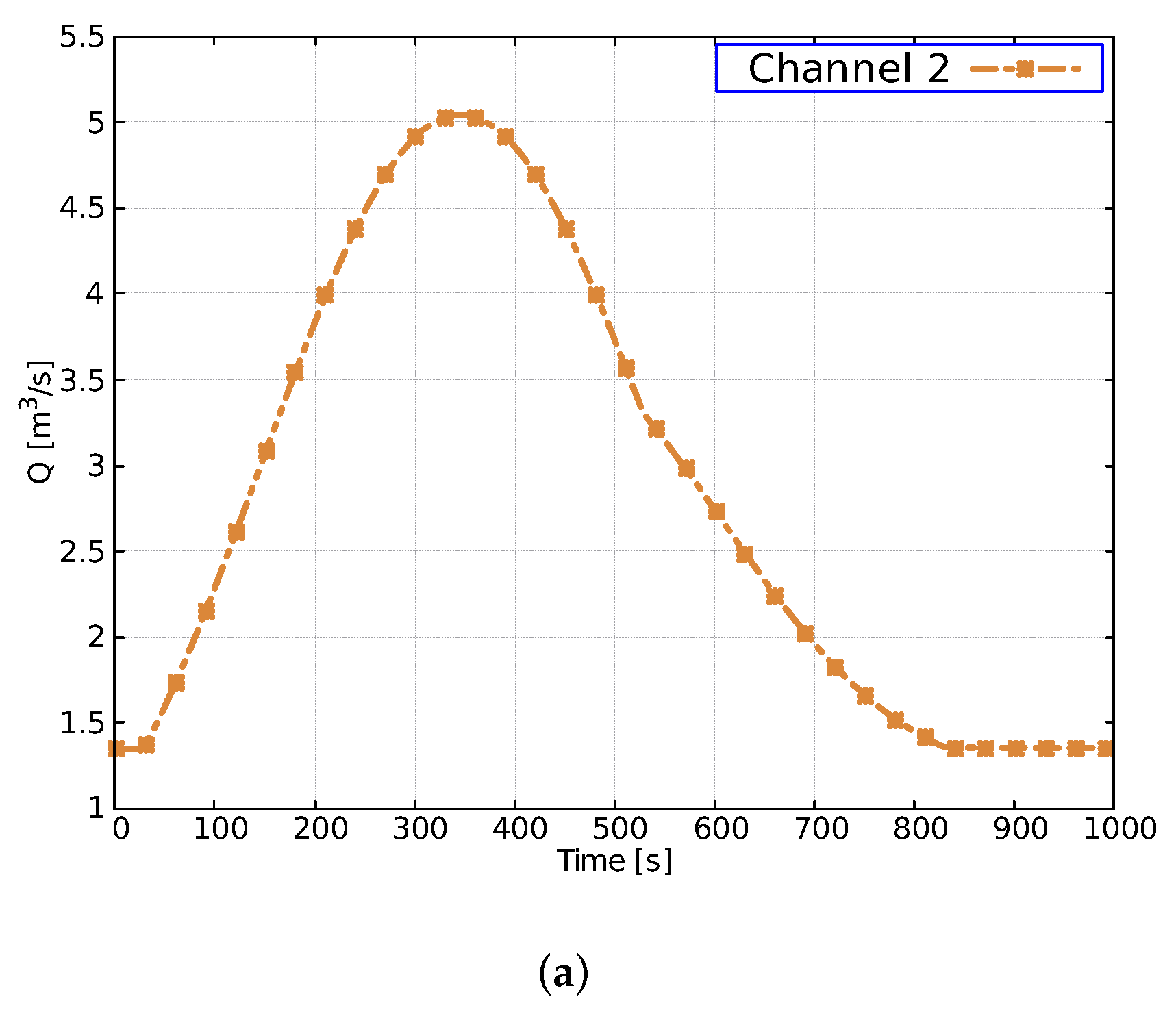
4.5. Case 6: Unsteady Flow with Two Solutes and Friction

In this case, two solutes ${\varphi }_1$ and ${\varphi }_2$ with different decay rates $k_{{\varphi }_1}$ and $k_{{\varphi }_2}$, respectively, are considered. The hydraulic characteristics (see Figure 4) include now slope and friction for all channels: $S_0=0.001$ and $n=0.035$ sm${}^{-1/3}$. The initial conditions for the flow are

$$\begin{array}{cc}\hfill & Q{(x,0)}_1=1.14{\mathrm{m}}^3/\mathrm{s}{\varphi }_1{(x,0)}_1=0\mathrm{g}/{\mathrm{m}}^3{\varphi }_2{(\mathrm{x},0)}_1=0\mathrm{g}/{\mathrm{m}}^3\mathrm{x}\in [0,{\mathrm{L}}_1]\hfill \\ \hfill & Q{(x,0)}_2=1.35{\mathrm{m}}^3/\mathrm{s}{\varphi }_1{(x,0)}_2=0\mathrm{g}/{\mathrm{m}}^3{\varphi }_2{(\mathrm{x},0)}_2=0\mathrm{g}/{\mathrm{m}}^3\mathrm{x}\in [0,{\mathrm{L}}_2]\hfill \\ \hfill & Q{(x,0)}_3=0.21{\mathrm{m}}^3/\mathrm{s}{\varphi }_1{(x,0)}_3=0\mathrm{g}/{\mathrm{m}}^3{\varphi }_2{(\mathrm{x},0)}_3=0\mathrm{g}/{\mathrm{m}}^3\mathrm{x}\in [0,{\mathrm{L}}_3]\hfill \end{array}$$

On the other hand, the flow boundary conditions for channels 1 and 3 are a transient configuration defined by (21) using $a_1=3,b_1=250,c_1=180$ for channel 1 and $a_3=2.5$, $b_3=400,c_3=180$ for channel 3. The theoretical solute upstream boundary conditions to be reconstructed are highlighted in grey in

Table 3. Case 6. Gaussian function parameters and decay rates of the three channels.

Channel	Variables
	${\mathit{\varphi }}_1(0,\mathit{t})$			${\mathit{\varphi }}_2(0,\mathit{t})$			Decay Rate (s${}^{-1}$)
	a	b	c	a	b	c	${\mathit{k}}_{{\mathit{\varphi }}_1}$	${\mathit{k}}_{{\mathit{\varphi }}_2}$
channel 1	2	250	30	4	250	30	$1\times {10}^{-5}$	$2\times {10}^{-2}$
channel 2		-			-		$4\times {10}^{-3}$	$2\times {10}^{-3}$
channel 3	1	400	30	2	400	30	$8\times {10}^{-6}$	$1.5\times {10}^{-6}$

and are also defined by Equation (22). The remaining parameters and the decay rates are defined in Table 3.

The measurement station is located downstream of the junctions at $x_M=35.5$ m in channel 2. The mesh size used in this test case is $\Delta x=1$ m, with a CFL = 1 and a step length $ϵ=10$. The numerical results are plotted in the Figure 11. Figure 11a shows the numerical solution of the flow measured at $x_M$ free of disturbances. Figure 11b,d displays the reconstructions of the inlet boundary condition for solutes ${\varphi }_1$ and ${\varphi }_2$, respectively, showing an acceptable convergence to a stable solution after 100 iterations.

Figure 11c,e shows the target for ${\varphi }_1$ and ${\varphi }_2$ after some iterations (dashed lines in colors), requiring 100 iterations to successfully converge to the registered downstream shape.

5. Discussion

This study presents a predictive explicit model for surface flow and transport of a non-conservative solute in a channel junction together with the adjoint formulation of the conservative and non-conservative transport equations. All the test cases used are synthetic and followed the channel network shown in Figure 4. In this section, the numerical results, the keys of the scheme, the combination of the hydrodynamic, transport, adjoint and first-order gradient models, and the limitations of the proposed strategy are analyzed.

The technique is completely stable under the CFL condition when considering the hydrodynamic source terms (slope and friction) and the source term of the adjoint and physical transport equation (decay rate). Together with appropriate junction boundary conditions, this technique is demonstrated to solve satisfactorily both steady state and unsteady scenarios in a channel junction.

Optimization models considered in the literature frequently require hundreds of calls of both the hydrodynamic and transport models to find the best accordance between computed and observed state variables (model components) by variation of a number of parameters [43,44], so a model with these features will require considerable computational burden. Among the different alternatives for the inverse modeling offered by predictive models, the adjoint formulation has demonstrated to be an efficient and flexible tool. This works explores the extension of the adjoint technique to reconstruct the solute boundary condition in hydrodynamic models with solute transport at junction of channels.

The adjoint equations are solved using the same numerical scheme, computational grid and time step size as the physical equations. Moreover, they are supplied with the hydrodynamic information previously stored in the first simulation. This allows the error to be transported from the measurement point to the control point. Consequently, the gradient is used in the optimization method, allowing the boundary condition to be reconstructed efficiently and with relevant accuracy in all the scenarios proposed in this work. This is justified by the value of the functional in the last iteration, generally reduced by a 99.9% factor.

The versatility of the method to reconstruct the information at different channels has also been demonstrated. This was evidenced in Case 4 where the convergence of the functional achieves satisfactory results in both cases (Figure 8b,d). These results are evidenced with the evaluation of the root mean square error (RMSE) of the reconstructed upstream boundary condition at the last iteration (see

Table 4. Root mean square error of the reconstructed boundary conditions.

Case	RMSE ($\mathbf{g}/{\mathbf{m}}^3$)
Case 1	0.02013
Case 2 MNC 100	0.0101
Case 2 MNC 200	0.0105
Case 2 MNC 400	0.0123
Case 2.1	0.208
Case 2.2	0.085
Case 2.3	0.034
Case 3.1	0.299
Case 3.2	0.3
Case 3.3	0.361
Case 3.4	0.298
Case 3.5	0.299
Case 3.6	0.301
Case 3.7	0.359
Case 3.8	0.299
Case 3.9	0.284
Case 3.10	0.196
Case 3.11	0.198
Case 3.12	0.314
Case 4	0.008
Case 5	0.154
Case 6	0.025

). The evaluation criterion used reveals that the predictive precision and the fit of the model by means of the adjoint method have a better performance when the solute transported in unsteady flow is Gaussian. For this case, an RMSE = 0.0088 $\mathrm{g}/{\mathrm{m}}^3$ is reached compared to an RMSE = 0.361 $\mathrm{g}/{\mathrm{m}}^3$ in Case 3.3 when the solute pulse is a stepwise function.

This work is an encouraging step forward to extend the method presented in [27] for water quality optimization analysis in branched channel or river networks. However, the main limitation of the model is the oscillatory trend for the reconstruction of a stepwise signal, leading to notable differences, especially in sudden changes in concentration. An example of this is Case 5, where the concentration varies sharply from 1 to 3 $\mathrm{g}/{\mathrm{m}}^3$ in a period of time of 1s (see Figure 10a). Another potential downside of the method is the necessity of storing of all the flow information in each computational cell and each time step. This downside could be overcome with techniques such as check pointing [45] which can be analyzed in future works of this nature.

6. Conclusions

This study reveals that the transport equation model can serve as a first step to understand the relationships between the channel network and the control of the concentration of a solute downstream junction. The results showed that the accuracy of the boundary condition reconstruction depends largely on the shape of the signal to be reconstructed. However, these variations can be reduced by refining the computational mesh and increasing the number of iterations. The numerical solutions also indicate that, as the measurement station moves away from the reconstruction point, the final functional value in the last iteration becomes larger. Furthermore, it is demonstrated that few iterations in both steady state and unsteady scenarios are required to reconstruct the inlet boundary conditions of one or more solutes at a time.

Finally, the efficiency of the technique requires that the same computational mesh, the hydrodynamic characteristics and time step size be used when solving the transport equation and the adjoint equation in the optimization process. Besides this restriction, the optimization model presented in this work has been proved to be robust, accurate and efficient for different hydrodynamic and solute configurations.

References

1. Chapra, S.C. Engineering water quality models and TMDLs. J. Water Resour. Plan. Manag. 2003, 129, 247–256. [Google Scholar] [CrossRef]
2. Garcia-Navarro, M.; Savirón, J. Numerical simulation of unsteady flow at open channel junctions. J. Hydraul. Res. 1992, 30, 595–609. [Google Scholar] [CrossRef]
3. Hsu, C.C.; Lee, W.J.; Chang, C.H. Subcritical open-channel junction flow. J. Hydraul. Eng. 1998, 124, 847–855. [Google Scholar] [CrossRef]
4. Best, J.; Roy, A. Mixing layer distortion at the confluence of unequal depth channels. Nature 1991, 350, 411–413. [Google Scholar] [CrossRef]
5. Best, J.L. Flow dynamics at river channel confluences: Implications for sediment transport and bed morphology. In Recent Developments in Fluvial Sedimentology, 39; Ethridge, F., Flores, M., Harvey, M., Eds.; Society of Economic Paleontologists and Mineralogists, Special Publication: Tulsa, OK, USA, 1987; pp. 27–35. [Google Scholar]
6. Best, J.L. Sediment transport and bed morphology at river channel confluences. Sedimentology 1988, 35, 481–498. [Google Scholar] [CrossRef]
7. Kenworthy, S.T.; Rhoads, B.L. Hydrologic control of spatial patterns of suspended sediment concentration at a stream confluence. J. Hydrol. 1995, 168, 251–263. [Google Scholar] [CrossRef]
8. Tong-Huan, L.; Yi-Kui, W.; Xie-Kang, W.; Huan-Feng, D.; Xu-Feng, Y. Morphological environment survey and hydrodynamic modeling of a large bifurcation-confluence complex in Yangtze River, China. Sci. Total Environ. 2020, 737, 139705. [Google Scholar]
9. Ghostine, R.; Vazquez, J.; Terfous, A.; Mose, R.; Ghenaim, A. Comparative study of 1D and 2D flow simulations at open-channel junctions. J. Hydraul. Res. 2012, 50, 164–170. [Google Scholar] [CrossRef]
10. Constantinescu, G.; Miyawaki, S.; Rhoads, B.; Sukhodolov, A. Numerical evaluation of the effects of planform geometry and inflow conditions on flow, turbulence structure, and bed shear velocity at a stream confluence with a concordant bed. J. Geophys. Res. Earth Surf. 2014, 119, 2079–2097. [Google Scholar] [CrossRef]
11. Constantinescu, G.; Miyawaki, S.; Rhoads, B.; Sukhodolov, A. Numerical analysis of the effect of momentum ratio on the dynamics and sediment-entrainment capacity of coherent flow structures at a stream confluence. J. Geophys. Res. F04028 2012, 117, F04028. [Google Scholar] [CrossRef]
12. Constantinescu, G.; Miyawaki, S.; Rhoads, B.; Sukhodolov, A.; Kirkil, G. Structure of turbulent flow at a river confluence with momentum and velocity ratios close to 1: Insight provided by an eddy-resolving numerical simulation. Water Resour. Res. 2011, 47, W05507. [Google Scholar] [CrossRef]
13. Gualtieri, C.; Filizola, N.; de Oliveira, M.; Santos, A.M.; Ianniruberto, M. A field study of the confluence between Negro and Solimões Rivers. Part 1: Hydrodynamics and sediment transport. Comptes Rendus Geosci. 2018, 350, 31–42. [Google Scholar] [CrossRef]
14. Ianniruberto, M.; Trevethan, M.; Pinheiro, A.; Andrade, J.F.; Dantas, E.; Filizola, N.; Santos, A.; Gualtieri, C. A field study of the confluence between Negro and Solimões Rivers. Part 2: Bed morphology and stratigraphy. Comptes Rendus Geosci. 2018, 350, 43–54. [Google Scholar] [CrossRef]
15. Burguete, J.; Zapata, N.; García-Navarro, P.; Maïkaka, M.; Playán, E.; Murillo, J. Fertigation in furrows and level furrow systems. I: Model description and numerical tests. J. Irrig. Drain. Eng. 2009, 135, 401–412. [Google Scholar] [CrossRef] [Green Version]
16. Tang, H.; Zhang, H.; Yuan, S. Hydrodynamics and contaminant transport on a degraded bed at a 90-degree channel confluence. Environ. Fluid Mech. 2018, 18, 443–463. [Google Scholar] [CrossRef]
17. Xiao, Y.; Xia, Y.; Yuan, S.y.; Tang, H.w. Flow structure and phosphorus adsorption in bed sediment at a 90° channel confluence. J. Hydrodyn. Ser. B 2017, 29, 902–905. [Google Scholar] [CrossRef]
18. Yuan, S.; Tang, H.; Xiao, Y.; Xia, Y.; Melching, C.; Li, Z. Phosphorus contamination of the surface sediment at a river confluence. J. Hydrol. 2019, 573, 568–580. [Google Scholar] [CrossRef]
19. Cheng, Z.; Constantinescu, G. Stratification effects on flow hydrodynamics and mixing at a confluence with a highly discordant bed and a relatively low velocity ratio. Water Resour. Res. 2018, 54, 4537–4562. [Google Scholar] [CrossRef]
20. Gualtieri, C.; Ianniruberto, M.; Filizola, N. On the mixing of rivers with a difference in density: The case of the Negro/Solimões confluence, Brazil. J. Hydrol. 2019, 578, 124029. [Google Scholar] [CrossRef]
21. Lacasta, A.; Morales-Hernández, M.; Brufau, P.; García-Navarro, P. Application of an adjoint-based optimization procedure for the optimal control of internal boundary conditions in the shallow water equations. J. Hydraul. Res. 2018, 56, 111–123. [Google Scholar] [CrossRef]
22. Neupauer, R.M. Adjoint sensitivity analysis of contaminant concentrations in water distribution systems. J. Eng. Mech. 2011, 137, 31–39. [Google Scholar] [CrossRef]
23. Piasecki, M. Optimal wasteload allocation procedure for achieving dissolved oxygen water quality objectives. I: Sensitivity analysis. J. Environ. Eng. 2004, 130, 1322–1334. [Google Scholar] [CrossRef]
24. Sanders, B.F.; Katopodes, N.D. Adjoint sensitivity analysis for shallow-water wave control. J. Eng. Mech. 2000, 126, 909–919. [Google Scholar] [CrossRef]
25. Katopodes, N.D. Free-Surface Flow: Environmental Fluid Mechanics; Butterworth-Heinemann: Oxford, UK, 2018. [Google Scholar]
26. Marchuk, G.I. Mathematical Models in Environmental Problems; Elsevier: Amsterdam, The Netherlands, 2011; Volume 16. [Google Scholar]
27. Gordillo, G.; Morales-Hernández, M.; García-Navarro, P. A gradient-descent adjoint method for the reconstruction of boundary conditions in a river flow nitrification model. Environ. Sci. Process. Impacts 2020, 22, 381–397. [Google Scholar] [CrossRef]
28. Kundu, P.; Cohen, I.; Dowling, D. Fluid Mechanics; Waltham: Singapore, 2012. [Google Scholar]
29. Chapra, S.C. Surface Water-Quality Modeling; Waveland Press: Long Grove, IL, USA, 2008; pp. 175–183. [Google Scholar]
30. Thomann, R.V.; Mueller, J.A. Principles of Surface Water Quality Modeling and Control; Harper & Row, Publishers: New York, NY, USA, 1987. [Google Scholar]
31. Ramezani, M.; Noori, R.; Hooshyaripor, F.; Deng, Z.; Sarang, A. Numerical modelling-based comparison of longitudinal dispersion coefficient formulas for solute transport in rivers. Hydrol. Sci. J. 2019, 64, 808–819. [Google Scholar] [CrossRef]
32. Cheme, E.K.; Mazaheri, M. The effect of neglecting spatial variations of the parameters in pollutant transport modeling in rivers. Environ. Fluid Mech. 2021, 21, 587–603. [Google Scholar] [CrossRef]
33. Abbott, M.; Minns, A. Computational Hydraulics: Elements of the Theory of Free Surface Flows; MB Abbott. Pitman Publishing: London, UK, 1979. [Google Scholar]
34. Ji, Z.G. Hydrodynamics and Water Quality: Modeling Rivers, Lakes, and Estuaries; John Wiley & Sons: Hoboken, NJ, USA, 2017. [Google Scholar]
35. Gordillo, G.; Morales-Hernández, M.; García-Navarro, P. Finite volume model for the simulation of 1D unsteady river flow and water quality based on the WASP. J. Hydroinform. 2020, 22, 327–345. [Google Scholar] [CrossRef]
36. Murillo, J.; Navas-Montilla, A. A comprehensive explanation and exercise of the source terms in hyperbolic systems using Roe type solutions. Application to the 1D-2D shallow water equations. Adv. Water Resour. 2016, 98, 70–96. [Google Scholar] [CrossRef] [Green Version]
37. Fernández-Pato, J.; Morales-Hernández, M.; García-Navarro, P. Implicit finite volume simulation of 2D shallow water flows in flexible meshes. Comput. Methods Appl. Mech. Eng. 2018, 328, 1–25. [Google Scholar] [CrossRef] [Green Version]
38. Morales-Hernández, M.; García-Navarro, P.; Burguete, J.; Brufau, P. A conservative strategy to couple 1D and 2D models for shallow water flow simulation. Comput. Fluids 2013, 81, 26–44. [Google Scholar] [CrossRef] [Green Version]
39. Morales-Hernández, M.; Murillo, J.; García-Navarro, P. Diffusion–dispersion numerical discretization for solute transport in 2D transient shallow flows. Environ. Fluid Mech. 2019, 19, 1217–1234. [Google Scholar] [CrossRef] [Green Version]
40. Fernández-Pato, J.; García-Navarro, P. Finite volume simulation of unsteady water pipe flow. Drink. Water Eng. Sci. 2014, 7, 83–92. [Google Scholar] [CrossRef] [Green Version]
41. Murillo, J.; García-Navarro, P. Weak solutions for partial differential equations with source terms: Application to the shallow water equations. J. Comput. Phys. 2010, 229, 4327–4368. [Google Scholar] [CrossRef]
42. Piasecki, M. Optimal wasteload allocation procedure for achieving dissolved oxygen water quality objectives. II: Optimal load control. J. Environ. Eng. 2004, 130, 1335–1344. [Google Scholar] [CrossRef]
43. Lacasta, A.; Morales-Hernández, M.; Burguete, J.; Brufau, P.; García-Navarro, P. Calibration of the 1D shallow water equations: A comparison of Monte Carlo and gradient-based optimization methods. J. Hydroinform. 2017, 19, 282–298. [Google Scholar] [CrossRef] [Green Version]
44. MIKE21, D.; MIKE3 Flow Model, F. Hydrodynamic and Transport Module Scientific Documentation; DHl Water & Environment: Hørsholm, Denmark, 2009. [Google Scholar]
45. Lacasta, A.; García-Navarro, P. A GPU accelerated adjoint-based optimizer for inverse modeling of the two-dimensional shallow water equations. Comput. Fluids 2016, 136, 371–383. [Google Scholar] [CrossRef]
Figure 1. Spatial domain of junctions.
Mathematics 10 00093 g001
Figure 2. Discretization of time and space in the adjoint equation.
Mathematics 10 00093 g002
Figure 3. Scheme to reconstruct the information of the boundary condition through the adjoint and gradient-descent method.
Mathematics 10 00093 g003
Figure 4. Case 1. Schematic of the three channels at a 90° confluence.
Mathematics 10 00093 g004
Figure 5. Case 1. Evolution of the reconstruction of the boundary condition (a) and evolution of the target (b) at some iterations.
Mathematics 10 00093 g005
Figure 6. Case 1. Reconstruction of the boundary condition at iteration 100 (a) and evolution of the objective function at each iteration (b) for different number of cells.
Mathematics 10 00093 g006
Figure 7. Case 3. Evolution of the reconstruction of the boundary condition (a) and evolution of the target (b) in some iterations.
Mathematics 10 00093 g007
Figure 8. Case 4. Evolution of the functional in the different proposed scenarios.
Mathematics 10 00093 g008
Figure 9. Case 5. Temporal evolution of flow-rate at x M , 2 = 5.5 m.
Mathematics 10 00093 g009
Figure 10. Case 5. Evolution of the reconstruction of the boundary condition (a) and evolution of the target (b) in some iterations.
Mathematics 10 00093 g010
Figure 11. Case 4. Temporal evolution of flow-rate at x M , 2 = 35.5 m (a) and reconstruction of the boundary condition ϕ 1 and ϕ 2 (b,d) and target at x M , 2 = 35.5 m (c,e).
Mathematics 10 00093 g011aMathematics 10 00093 g011b