Some New Hermite-Hadamard-Fejér Fractional Type Inequalities for h-Convex and Harmonically h-Convex Interval-Valued Functions

Abstract

In this article, firstly, we establish a novel definition of weighted interval-valued fractional integrals of a function $\breve{\mathsf{{\rm Y}}}$ using an another function $\vartheta \left(\dot{\zeta }\right)$. As an additional observation, it is noted that the new class of weighted interval-valued fractional integrals of a function $\breve{\mathsf{{\rm Y}}}$ by employing an additional function $\vartheta \left(\dot{\zeta }\right)$ characterizes a variety of new classes as special cases, which is a generalization of the previous class. Secondly, we prove a new version of the Hermite-Hadamard-Fejér type inequality for h-convex interval-valued functions using weighted interval-valued fractional integrals of a function $\breve{\mathsf{{\rm Y}}}$ according to another function $\vartheta \left(\dot{\zeta }\right).$ Finally, by using weighted interval-valued fractional integrals of a function $\breve{\mathsf{{\rm Y}}}$ according to another function $\vartheta \left(\dot{\zeta }\right)$, we are establishing a new Hermite-Hadamard-Fejér type inequality for harmonically h-convex interval-valued functions that is not previously known. Moreover, some examples are provided to demonstrate our results.

1. Introduction

Mathematicians use convex functions in many fields, such as optimization and advanced analysis. Convex functions offer several unique qualities, such as a unique minimum on an open set if strictly convex. Moreover, convex functions have identical qualities even when the spatial dimension is not finite, and as a result, they are instances of functionals in variation methods. In the theory of probability, a convex function obtained through the use of a random variable is constrained above by the expected value. Numerous inequalities are established for convex functions, but the Hermite-Hadamard inequality is the most well-known from the relevant literature. A function $\breve{\mathsf{{\rm Y}}}:[{\ell }_1,{\ell }_2]\subset \mathbb{R}\to \mathbb{R}$ is called convex, if for all ${\ell }_1,{\ell }_2\in I$ and $\dot{\zeta }\in [0,1]$, then

$$\breve{\mathsf{{\rm Y}}}(\dot{\zeta }{\ell }_1+(1-\dot{\zeta }){\ell }_2)\le \dot{\zeta }\breve{\mathsf{{\rm Y}}}\left({\ell }_1\right)+(1-\dot{\zeta })\breve{\mathsf{{\rm Y}}}\left({\ell }_2\right).$$

(1)

An famous mathematical inequality in the field of convex functional analysis is the Hermite-Hadamard integral inequality. It has an intriguing geometric representation and a wide variety of significant applications. According to the remarkable inequality, if considering a convex function $\breve{\mathsf{{\rm Y}}}:I\to \mathbb{R}$ and ${\ell }_1,{\ell }_2\in I$ with ${\ell }_1<{\ell }_2,$ then

$$\breve{\mathsf{{\rm Y}}}\left(\frac{{\ell }_1+{\ell }_2}{2}\right)\le \frac{1}{{\ell }_2-{\ell }_1}\underset{{\ell }_1}{\overset{{\ell }_2}{\int }}\breve{\mathsf{{\rm Y}}}\left(\dot{\zeta }\right)d\dot{\zeta }\le \frac{\breve{\mathsf{{\rm Y}}}\left({\ell }_1\right)+\breve{\mathsf{{\rm Y}}}\left({\ell }_2\right)}{2}.$$

(2)

C. Hermite [1] presented inequality (2) in 1893, and J. Hadamard [2] explored it. If $\breve{\mathsf{{\rm Y}}}$ is concave, these inequalities are true in the reversed direction. Numerous mathematicians have concentrated their attention on the Hermite-Hadamard inequality because of its superiority and integrity in the field of mathematical inequalities. For key improvements, extensions, and applications of the Hermite-Hadamard uniqueness theorem and basic convex function definitions, for key details, please see [3,4,5] and references therein.

Fractional calculus is currently focused on the research of so-called fractional order integral and derivative functions over real and complex domains and their applications. The use of arithmetic from classical analysis in fractional analysis is critical for achieving more realistic findings in the solution of many problems. Numerous mathematical models are properly handled by differential equations of fractional order. A fractional mathematical model has more general and accurate findings than classical mathematical models, because they are specific examples of fractional order mathematical models. In classical analysis, integer orders aren’t a good model for nature. Fractional computation, on the other hand, lets us look at any number of orders and come up with much more quantitative objectives. Concerning several publications that deal with fractional integral inequalities using various forms of fractional integral operators. The reader who is interested might like to refer to [6,7,8,9,10,11,12,13,14,15,16,17,18,19,20,21,22,23,24,25,26,27] and references therein.

However, interval analysis is a remarkable example of set-valued analysis, which is the research of sets following both mathematical analysis and basic topology as a technique for dealing with interval uncertainty, which can be present in many statistical or computer models of deterministic real-world behaviors. The Archimedes method, which is used to calculate the circumference of a circle, is a historical example of an interval enclosure. In [28], Moore, who is credited with being the first person to apply intervals in computer mathematics, published the first book on interval analysis in 1966, which is still in print today. After his book was published, many scientists began investigating the theory and applications of interval arithmetic, prompting him to issue a second edition. The use of interval analysis has become increasingly popular in recent years, thanks to its many practical applications in a wide range of fields that are very interested in ambiguous data. A wide range of applications can be found in computer graphics, experimental physics, computational physics, error analysis, and robotics. The interested reader is advised to consult the citations [29,30,31,32] and the references therein for the most important details.

2. Interval Calculus

Throughout this section, we will present the used notation as well as some basic knowledge of interval analysis and its applications. Considering the space of all closed intervals of $\mathbb{R}$ denoted by ${\mathbb{R}}_I$ and $\widehat{\mathcal{Q}}$ as a bounded element of ${\mathbb{R}}_I$, we have the representation

$$\widehat{\mathcal{Q}}=\left[\underline{\gamma },\overline{\gamma }\right]=\left\{\dot{\zeta }\in \mathbb{R}:\underline{\gamma }\le \dot{\zeta }\le \overline{\gamma }\right\}$$

where $\underline{\gamma },\overline{\gamma }\in \mathbb{R}$ and $\underline{\gamma }\le \overline{\gamma }.$ This is the length of the $=\left[\underline{\gamma },\overline{\gamma }\right]$ that may be expressed as $\mathcal{L}\left(\widehat{\mathcal{Q}}\right)=\overline{\gamma }-\underline{\gamma }.$ The values $\underline{\gamma }$ and $\overline{\gamma }$ are referred to as the left and right ends of the interval $\widehat{\mathcal{Q}},$ respectively. As a result, the interval $\widehat{\mathcal{Q}}$ is said to be degenerate when $\overline{\gamma }=\underline{\gamma }=q.$ In this case, we use the mathematical expression $\widehat{\mathcal{Q}}=q=[q,q]$. Another way to express this is to say that $\widehat{\mathcal{Q}}$ is positive if $\underline{\gamma }$ is greater than zero or that $\widehat{\mathcal{Q}}$ is negative if $\overline{\gamma }$ is less than zero. The sets of all closed positive and negative intervals of $\mathbb{R}$ are represented by ${\mathbb{R}}_I^{+}$ and ${\mathbb{R}}_I^{-},$ respectively. The Pompeiu-Hausdorff distance is defined as the distance between the intervals $\widehat{\mathcal{Q}}$ and $\widehat{\mathcal{T}}$.

$$d_H\left(\widehat{\mathcal{Q}},\widehat{\mathcal{T}}\right)=d_H\left(\left[\underline{\gamma },\overline{\gamma }\right],\left[\underline{\zeta },\overline{\zeta }\right]\right)=max\left\{\left|\underline{\gamma }-\underline{\zeta }\right|,\left|\overline{\gamma }-\overline{\zeta }\right|\right\}.$$

(3)

In mathematics, the metric space $\left({\mathbb{R}}_I,d\right)$ is recognized to be a complete metric space (see [8]).

Specifically, its absolute value is denoted by the symbol $|\widehat{\mathcal{Q}}|$, and mathematically it is defined as follows:

$$\left|\widehat{\mathcal{Q}}\right|=max\left\{\left|\underline{\gamma }\right|,\left|\overline{\gamma }\right|\right\}.$$

Furthermore, given the intervals $\widehat{\mathcal{Q}}$ and $\widehat{\mathcal{T}}$, the definitions of basic interval arithmetic techniques are as follows:

$$\begin{array}{ccc}\hfill \widehat{\mathcal{Q}}+\widehat{\mathcal{T}}& =\left[\underline{\gamma }+\underline{\zeta },\overline{\gamma }+\overline{\zeta }\right],\hfill & \\ \hfill \widehat{\mathcal{Q}}-\widehat{\mathcal{T}}& =\left[\underline{\gamma }-\overline{\zeta },\overline{\gamma }-\underline{\zeta }\right],\hfill & \\ \hfill \widehat{\mathcal{Q}}·\widehat{\mathcal{T}}& =\left[min\widehat{\mathcal{U}},max\widehat{\mathcal{U}}\right]\mathrm{where}\widehat{\mathcal{U}}=\left\{\underline{k}\underline{\zeta },\underline{\gamma }\overline{\zeta ,}\overline{\gamma }\underline{\zeta },\overline{\gamma }\overline{\zeta }\right\},\hfill & \\ \hfill \widehat{\mathcal{Q}}/\widehat{\mathcal{T}}& =\left[min\widehat{\mathcal{V}},max\widehat{\mathcal{V}}\right]\mathrm{where}\widehat{\mathcal{V}}=\left\{\underline{\gamma }/\underline{\zeta },\underline{\gamma }/\overline{\zeta },\overline{\gamma }/\underline{\zeta },\overline{\gamma }/\overline{\zeta }\right\}\mathrm{and}0\notin \widehat{\mathcal{T}}.\hfill \end{array}$$

The interval $\widehat{\mathcal{Q}}$ is scalar multiplied by

$$\eta \widehat{\mathcal{Q}}=\eta \left[\underline{\gamma },\overline{\gamma }\right]=\left\{\begin{array}{cc}\left[\eta \underline{\gamma },\eta \overline{\gamma }\right],\hfill & \eta >0;\hfill \\ & \\ \left\{0\right\},\hfill & \eta =0;\hfill \\ & \\ \left[\eta \overline{\gamma },\eta \underline{\gamma }\right],\hfill & \eta <0,\hfill \end{array}\right.$$

where $\eta \in \mathbb{R}.$

The interval $\widehat{\mathcal{Q}}$ is the inverse

$$-\widehat{\mathcal{Q}}:=(-1)\widehat{\mathcal{Q}}=[-\overline{\gamma },-\underline{\gamma }],$$

where $\eta =-1$.

The subtraction is denoted by the symbol

$$\widehat{\mathcal{Q}}-\widehat{\mathcal{T}}=\widehat{\mathcal{Q}}+(-\widehat{\mathcal{T}})=[\underline{\gamma }-\overline{\zeta },\overline{\gamma }-\underline{\zeta }].$$

Consequently, $-\widehat{\mathcal{Q}}$ is not an additive inverse for $\widehat{\mathcal{Q}},$ so, $\widehat{\mathcal{Q}}-\widehat{\mathcal{Q}}\ne 0.$

The definitions of operations result in a large number of algebraic characteristics, which allow ${\mathbb{R}}_I$ to be a quasilinear space (see, [9]).

(1)

(Associativity of addition) $(\widehat{\mathcal{Q}}+\widehat{\mathcal{T}})+\widehat{\mathcal{S}}=$ $\widehat{\mathcal{Q}}+(\widehat{\mathcal{T}}+\widehat{\mathcal{S}})$ for all $\widehat{\mathcal{Q}},\widehat{\mathcal{T}},\widehat{\mathcal{S}}\in {\mathbb{R}}_I,$

(2)

(Additivity element) $\widehat{\mathcal{Q}}+0=0+\widehat{\mathcal{Q}}=\widehat{\mathcal{Q}}$ for all $\widehat{\mathcal{Q}}\in {\mathbb{R}}_I,$

(3)

(Commutativity of addition) $\widehat{\mathcal{Q}}+\widehat{\mathcal{T}}=\widehat{\mathcal{T}}+\widehat{\mathcal{Q}}$ for all $\widehat{\mathcal{Q}},\widehat{\mathcal{T}}\in {\mathbb{R}}_I,$

(4)

(Cancellation law) $\widehat{\mathcal{Q}}+\widehat{\mathcal{S}}=\widehat{\mathcal{T}}+\widehat{\mathcal{S}}⟹\widehat{\mathcal{Q}}=\widehat{\mathcal{T}}$ for all $\widehat{\mathcal{Q}},\widehat{\mathcal{T}},\widehat{\mathcal{S}}\in {\mathbb{R}}_I,$

(5)

(Associativity of multiplication) $(\widehat{\mathcal{Q}}·\widehat{\mathcal{T}})·\widehat{\mathcal{S}}=\widehat{\mathcal{Q}}·(\widehat{\mathcal{T}}·\widehat{\mathcal{S}})$ for all $\widehat{\mathcal{Q}},\widehat{\mathcal{T}},\widehat{\mathcal{S}}\in {\mathbb{R}}_I,$

(6)

(Commutativity of multiplication) $\widehat{\mathcal{Q}}·\widehat{\mathcal{T}}=\widehat{\mathcal{T}}·\widehat{\mathcal{Q}}$ for all $\widehat{\mathcal{Q}},\widehat{\mathcal{T}}\in {\mathbb{R}}_I,$

(7)

(Unity element) $\widehat{\mathcal{Q}}·1=1·\widehat{\mathcal{Q}}$ for all $\widehat{\mathcal{Q}}\in {\mathbb{R}}_I,$

(8)

(Associativity law) $\lambda \left(\eta \widehat{\mathcal{Q}}\right)=\left(\lambda \eta \right)\widehat{\mathcal{Q}}$ for all $\widehat{\mathcal{Q}}\in {\mathbb{R}}_I$ and all $\lambda ,\eta \in \mathbb{R},$

(9)

(First distributivity law) $\lambda (\widehat{\mathcal{Q}}+\widehat{\mathcal{T}})=\lambda \widehat{\mathcal{Q}}+\lambda \widehat{\mathcal{T}}$ for all $\widehat{\mathcal{Q}},\widehat{\mathcal{T}}\in {\mathbb{R}}_I$ and all $\lambda \in \mathbb{R},$

(10)

(Second distributivity law) $(\lambda +\eta )\widehat{\mathcal{Q}}=\lambda \widehat{\mathcal{Q}}+\eta \widehat{\mathcal{Q}}$ for all $\widehat{\mathcal{Q}}\in {\mathbb{R}}_I$ and all $\lambda ,\eta \in \mathbb{R}.$

In addition to all these features, the distributive law is not always true for intervals. As an example, $\widehat{\mathcal{Q}}=[2,3],\widehat{\mathcal{T}}=[4,5]$ and $\widehat{\mathcal{S}}=[-4,-1].$

$$\widehat{\mathcal{Q}}·\left(\widehat{\mathcal{T}}+\widehat{\mathcal{S}}\right)=[0,12],$$

whereas

$$\widehat{\mathcal{Q}}·\widehat{\mathcal{T}}+\widehat{\mathcal{Q}}·\widehat{\mathcal{S}}=[0,12].$$

Definition 1

([9]). We represent the $g\widehat{\hslash }$-difference between $\widehat{\mathcal{Q}}$ and $\widehat{\mathcal{T}}$ as the interval $\widehat{\mathcal{M}}$ such that

$$\widehat{\mathcal{Q}}{\ominus }_g\widehat{\mathcal{T}}=\widehat{\mathcal{M}}\iff \left\{\begin{array}{c}\widehat{\mathcal{Q}}=\widehat{\mathcal{T}}+\widehat{\mathcal{M}},\\ or\\ \widehat{\mathcal{M}}=\widehat{\mathcal{Q}}+\left(-\widehat{\mathcal{T}}\right).\end{array}\right.$$

It appears to be unquestionable that

$$\widehat{\mathcal{Q}}{\ominus }_g\widehat{\mathcal{T}}=\left\{\begin{array}{c}\left[\underline{\gamma }-\underline{\zeta },\overline{\gamma }-\overline{\zeta }\right],if\mathcal{L}\left(\widehat{\mathcal{Q}}\right)\ge \mathcal{L}\left(\widehat{\mathcal{T}}\right),\\ \left[\overline{\gamma }-\overline{\zeta },\underline{\gamma }-\underline{\zeta }\right],if\mathcal{L}\left(\widehat{\mathcal{Q}}\right)<\mathcal{L}\left(\widehat{\mathcal{T}}\right).\end{array}\right.$$

Particularly, if $\widehat{\mathcal{T}}=\zeta \in \mathbb{R}$ is a constant, we have

$$\widehat{\mathcal{Q}}{\ominus }_g\widehat{\mathcal{T}}=\left[\underline{\gamma }-\zeta ,\overline{\gamma }-\zeta \right].$$

Additionally, another set property is the inclusion of ⊆, which is defined by

$$\widehat{\mathcal{Q}}\subseteq \widehat{\mathcal{T}}⟺\underline{\gamma }\le \underline{\zeta }\mathrm{and}\overline{\gamma }\le \overline{\zeta }.$$

3. Integral for Interval-Valued Functions

For a description of the fundamental ideas and definitions of interval analysis. see [11]. The concept of integral for interval-valued functions is discussed in this section. The following concepts must be understood before the definition of integral can be presented: $\breve{\mathsf{{\rm Y}}}$ is an interval-valued function of $[{\ell }_1,{\ell }_2]$, if it gives each a nonempty interval $\dot{\zeta }\in [{\ell }_1,{\ell }_2]$

$$\breve{\mathsf{{\rm Y}}}\left(\dot{\zeta }\right)=\left[\underline{\breve{\mathsf{{\rm Y}}}}\left(\dot{\zeta }\right),\overline{\breve{\mathsf{{\rm Y}}}}\left(\dot{\zeta }\right)\right].$$

A division of the numbers $[{\ell }_1,{\ell }_2]$ is any finite ordered subset of $\widehat{\mathcal{P}}$ that has the form

$$\widehat{\mathcal{P}}:{\ell }_1={\dot{\zeta }}_0<{\dot{\zeta }}_1\cdots <{\dot{\zeta }}_m={\ell }_2.$$

It is possible to define the mesh of a partition $\widehat{\mathcal{P}}$ as

$$mesh\left(\widehat{\mathcal{P}}\right)=max\{{\dot{\zeta }}_d-{\dot{\zeta }}_{d-1}:d=[1,m]\}.$$

The collection of all partitions of $[{\ell }_1,{\ell }_2]$ is denoted as $\widehat{\mathcal{P}}\left([{\ell }_1,{\ell }_2]\right).$ Suppose that $\widehat{\mathcal{P}}(\dot{\delta },[{\ell }_1,{\ell }_2])$ is the set of all $\widehat{\mathcal{P}}\in \widehat{\mathcal{P}}\left([{\ell }_1,{\ell }_2]\right)$ with property $mesh\left(\widehat{\mathcal{P}}\right)<\dot{\delta }$. Select an arbitrarily large point ${\xi }_i$ from the interval $[{\dot{\zeta }}_{d-1},{\dot{\zeta }}_d]$, ($d=[1,m]$) and now the sum is

$$\mathcal{S}(\breve{\mathsf{{\rm Y}}},\widehat{\mathcal{P}},\dot{\delta })=\sum _{d=1}^m\breve{\mathsf{{\rm Y}}}\left({\xi }_d\right)[{\dot{\zeta }}_d-{\dot{\zeta }}_{d-1}],$$

where $\breve{\mathsf{{\rm Y}}}:[{\ell }_1,{\ell }_2]\to {\mathbb{R}}_I$. We refer to this as $\mathcal{S}(\breve{\mathsf{{\rm Y}}},\widehat{\mathcal{P}},\dot{\delta })$ is a Riemann sum of $\breve{\mathsf{{\rm Y}}}$ matching to $\widehat{\mathcal{P}}\in \widehat{\mathcal{P}}(\dot{\delta },[{\ell }_1,{\ell }_2])$.

Definition 2.

Let $\breve{\mathsf{{\rm Y}}}:[{\ell }_1,{\ell }_2]\to {\mathbb{R}}_I$ be an interval Riemann integrable $\left(\right(\mathcal{IR})$-integrable) on $[{\ell }_1,{\ell }_2]$, if $\Delta \in {\mathbb{R}}_I$ then for any $ϵ>0$ and if $\dot{\delta }>0,$ then we have

$$d\left(\mathcal{S}(\breve{\mathsf{{\rm Y}}},\widehat{\mathcal{P}},\dot{\delta }),\Delta \right)<ϵ$$

or every Riemann sum $\mathcal{S}$ of $\breve{\mathsf{{\rm Y}}}$ corresponding to each $\widehat{\mathcal{P}}\in \widehat{\mathcal{P}}(dot\delta ,[{\ell }_1,{\ell }_2])$ and in addition to being independent of the $q_d\in [{\dot{\zeta }}_{d-1},{\dot{\zeta }}_d]$$\forall d=[1,m]$. This is referred to as the Δ is said the $\left(\mathcal{IR}\right)$-integral of $\breve{\mathsf{{\rm Y}}}$ on $[{\ell }_1,{\ell }_2]$ and is indicated by

$$\Delta =\left(\mathcal{IR}\right){\int }_{{\ell }_1}^{{\ell }_2}\breve{\mathsf{{\rm Y}}}\left(\dot{\zeta }\right)d\dot{\zeta }.$$

In this case, the collection of all functions that are $\left(\mathcal{IR}\right)$-integrable on $[{\ell }_1,{\ell }_2]$ will be designated by the symbol ${\mathcal{IR}}_{\left([{\ell }_1,{\ell }_2]\right)}$.

The theorem that follows establishes a relationship between $\left(\mathcal{IR}\right)$-integrable and Riemann integrable ($\mathcal{R}$-integrable function ):

Theorem 1.

Suppose that an interval-valued function $\breve{\mathsf{{\rm Y}}}:[{\ell }_1,{\ell }_2]\to {\mathbb{R}}_I$ and $\breve{\mathsf{{\rm Y}}}\left(\dot{\zeta }\right)=[\underline{\breve{\mathsf{{\rm Y}}}}\left(\dot{\zeta }\right),\overline{\breve{\mathsf{{\rm Y}}}}\left(\dot{\zeta }\right)]$. $\breve{\mathsf{{\rm Y}}}\in {\mathcal{IR}}_{\left([{\ell }_1,{\ell }_2]\right)}$ iff $\underline{\breve{\mathsf{{\rm Y}}}}\left(\dot{\zeta }\right),\overline{\breve{\mathsf{{\rm Y}}}}\left(\dot{\zeta }\right)\in {\mathcal{R}}_{\left([{\ell }_1,{\ell }_2]\right)}$ and

$$\left(\mathcal{IR}\right){\int }_{{\ell }_1}^{{\ell }_2}\breve{\mathsf{{\rm Y}}}\left(\dot{\zeta }\right)d\dot{\zeta }=\left[\left(\mathcal{R}\right){\int }_{{\ell }_1}^{{\ell }_2}\underline{\breve{\mathsf{{\rm Y}}}}\left(\dot{\zeta }\right)d\dot{\zeta },\left(\mathcal{R}\right){\int }_{{\ell }_1}^{{\ell }_2}\overline{\breve{\mathsf{{\rm Y}}}}\left(\dot{\zeta }\right)d\dot{\zeta }\right],$$

where ${\mathcal{R}}_{\left([{\ell }_1,{\ell }_2]\right)}$ represents the set of $\mathcal{R}$-integrable functions on the right side of the equation.

It is clear that if $\breve{\mathsf{{\rm Y}}}\left(\dot{\zeta }\right)\subseteq \mathcal{G}\left(\dot{\zeta }\right)$$\forall \dot{\zeta }\in [{\ell }_1,{\ell }_2]$, then

$$\left(\mathcal{IR}\right){\int }_{{\ell }_1}^{{\ell }_2}\breve{\mathsf{{\rm Y}}}\left(\dot{\zeta }\right)d\subseteq \left(\mathcal{IR}\right){\int }_{{\ell }_1}^{{\ell }_2}\mathcal{G}\left(\dot{\zeta }\right)d$$

Definition 3.

Let $\breve{\mathsf{{\rm Y}}}:[{\ell }_1,{\ell }_2]\to {\mathbb{R}}_I$ be an interval-valued function and $\breve{\mathsf{{\rm Y}}}\in {\mathcal{IR}}_{\left([{\ell }_1,{\ell }_2]\right)}.$ So, ${\mathcal{I}}_{{\ell }_1^{+}}^v$ is left-side and ${\mathcal{I}}_{{\ell }_2^{-}}^v$ is the right-sided interval Riemann-Liouville fractional integrals with order $v>0$, which is proved in [10]

$$\begin{array}{cc}\hfill & {\mathcal{I}}_{{\ell }_1^{+}}^v\breve{\mathsf{{\rm Y}}}\left(\dot{\zeta }\right)=\frac{1}{\Gamma \left(v\right)}\left(\mathcal{IR}\right)\underset{{\ell }_1}{\overset{\dot{\zeta }}{\int }}{(\dot{\zeta }-\kappa )}^{v-1}\breve{\mathsf{{\rm Y}}}\left(\kappa \right)d\kappa ,\dot{\zeta }>{\ell }_1,\hfill \\ \hfill & {\mathcal{I}}_{{\ell }_2^{-}}^v\breve{\mathsf{{\rm Y}}}\left(\dot{\zeta }\right)=\frac{1}{\Gamma \left(v\right)}\left(\mathcal{IR}\right)\underset{\dot{\zeta }}{\overset{{\ell }_2}{\int }}{(\kappa -\dot{\zeta })}^{v-1}\breve{\mathsf{{\rm Y}}}\left(\kappa \right)d\kappa ,\dot{\zeta }<{\ell }_2.\hfill \end{array}$$

respectively. Here, $\Gamma \left(v\right)$ is the Gamma function and ${\mathcal{I}}_{{\ell }_1^{+}}^0\breve{\mathsf{{\rm Y}}}\left(\dot{\zeta }\right)={\mathcal{I}}_{{\ell }_2^{-}}^0\breve{\mathsf{{\rm Y}}}\left(\dot{\zeta }\right)=\breve{\mathsf{{\rm Y}}}\left(\dot{\zeta }\right).$

In [11], Zhao et al. gave a definition of interval h-convex functions as follows:

Definition 4.

Suppose that a function $h:[0,1]\to {\mathbb{R}}^{+}$ and $\breve{\mathsf{{\rm Y}}}:[{\ell }_1,{\ell }_2]\to {\mathbb{R}}_I^{+}$ is called h-convex interval function, moreover the behavior of function $\breve{\mathsf{{\rm Y}}}$ be like that $\breve{\mathsf{{\rm Y}}}\in {\mathcal{IR}}_{\left([{\ell }_1,{\ell }_2]\right)}$, if for all ${\pi }_1,{\pi }_2\in [{\ell }_1,{\ell }_2]$ and $\dot{\zeta }\in [0,1]$, we have

$$\breve{\mathsf{{\rm Y}}}(\dot{\zeta }{\pi }_1+(1-\dot{\zeta }){\pi }_2)\supseteq h\left(\dot{\zeta }\right)\breve{\mathsf{{\rm Y}}}\left({\pi }_1\right)+h(1-\dot{\zeta })\breve{\mathsf{{\rm Y}}}\left({\pi }_2\right).$$

I. G. Macdonald provided the definition below in [12]:

Definition 5.

Let $\mathcal{G}:[{\ell }_1,{\ell }_2]\to [0,\infty )$ is a function and it is symmetric with respect to $\frac{{\ell }_1+{\ell }_2}{2}$ if

$$\mathcal{G}({\ell }_1+{\ell }_2-\kappa )=\mathcal{G}\left(\kappa \right),forall\kappa \in [{\ell }_1,{\ell }_2].$$

In [13], Zhao et al. gave a definition of interval h-harmonically convex functions as follows:

Definition 6.

Let $h:[0,1]\to {\mathbb{R}}^{+}$ be a non-negative function. We say that $\breve{\mathsf{{\rm Y}}}:[{\ell }_1,{\ell }_2]\to {\mathbb{R}}_I^{+}$ is interval h-harmonically convex function or that $\breve{\mathsf{{\rm Y}}}\in {\mathcal{IR}}_{\left([{\ell }_1,{\ell }_2]\right)}$, if for all ${\pi }_1,{\pi }_2\in [{\ell }_1,{\ell }_2]$ and $\dot{\zeta }\in [0,1]$, we have

$$\breve{\mathsf{{\rm Y}}}\left(\frac{{\pi }_1{\pi }_2}{\dot{\zeta }{\pi }_1+(1-\dot{\zeta }){\pi }_2}\right)\supseteq h(1-\dot{\zeta })\breve{\mathsf{{\rm Y}}}\left({\pi }_1\right)+h\left(\dot{\zeta }\right)\breve{\mathsf{{\rm Y}}}\left({\pi }_2\right).$$

In [14] Latif et. al. gave the following definition.

Definition 7.

A function $\breve{\mathsf{{\rm Y}}}:[{\ell }_1,{\ell }_2]\subseteq \mathbb{R}\backslash \left\{0\right\}\to \mathbb{R}$ is said to be harmonically symmetric with respect to $\frac{2{\ell }_1{\ell }_2}{{\ell }_1+{\ell }_2},$ if

$$\breve{\mathsf{{\rm Y}}}\left(\frac{1}{\kappa }\right)=\breve{\mathsf{{\rm Y}}}\left(\frac{1}{\frac{1}{{\ell }_1}+\frac{1}{{\ell }_2}-\kappa }\right),$$

$\kappa \in [{\ell }_1,{\ell }_2].$

In [15], according to Fejér proposal the Hadamard inequality can be generalized in the following ways:

Theorem 2.

Let $\breve{\mathsf{{\rm Y}}}:[{\ell }_1,{\ell }_2]\to \mathbb{R}$ be a convex function such that ${\ell }_1<{\ell }_2$. Also let $\mathcal{G}:[{\ell }_1,{\ell }_2]\to \mathbb{R}$ be a positive, integrable and symmetric to $\frac{{\ell }_1+{\ell }_2}{2}$. Then the following inequality holds:

$$\breve{\mathsf{{\rm Y}}}\left(\frac{{\ell }_1+{\ell }_2}{2}\right){\int }_{{\ell }_1}^{{\ell }_2}\mathcal{G}\left(\dot{\zeta }\right)d\dot{\zeta }\le {\int }_{{\ell }_1}^{{\ell }_2}\breve{\mathsf{{\rm Y}}}\left(\dot{\zeta }\right)\mathcal{G}\left(\dot{\zeta }\right)d\dot{\zeta }\le \frac{\breve{\mathsf{{\rm Y}}}\left({\ell }_1\right)+\breve{\mathsf{{\rm Y}}}\left({\ell }_2\right)}{2}{\int }_{{\ell }_1}^{{\ell }_2}\mathcal{G}\left(\dot{\zeta }\right)d\dot{\zeta }.$$

(4)

The inequality (4) is well-known in literature as in the Fejér-Hadamard inequality.

The main objective of this paper is to establish a new definition of weighted interval-valued fractional integrals of a function $\breve{\mathsf{{\rm Y}}}$ using an another function $\vartheta \left(\dot{\zeta }\right)$. 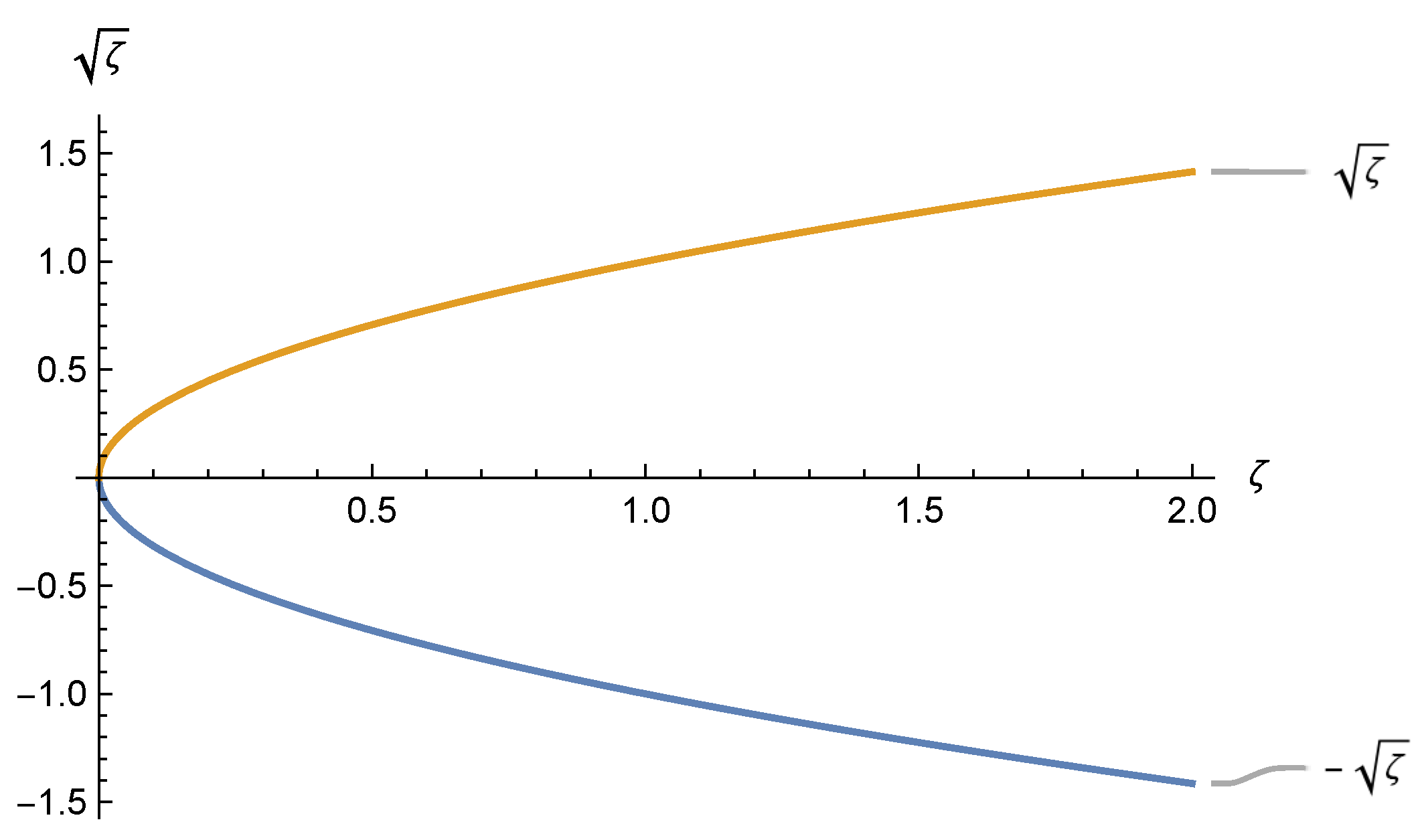Moreover, we prove a new version of the Hermite-Hadamard-Fejér type inequality for harmonically h-convex and h-convex interval-valued functions by applying weighted interval-valued fractional integrals of a function $\breve{\mathsf{{\rm Y}}}$ according to another function $\vartheta \left(\dot{\zeta }\right).$ Finally, new examples are calculated to verify our results, Figure 1 and Figure 2 are shown the graphical behavior of our results.

4. Auxiliary Results

In this section, we will define weighted left-side and right-side interval-valued fractional integrals of a function $\breve{\mathsf{{\rm Y}}}$ according to another function $\vartheta \left(\dot{\zeta }\right)$. Moreover, we will prove weighted symmetric interval-valued functions for h-convex and harmonically h-convex interval-valued functions.

Definition 8.

let $\breve{\mathsf{{\rm Y}}}:[{\ell }_1,{\ell }_2]\to {\mathbb{R}}_I^{+}$ be an interval-valued function such that $\breve{\mathsf{{\rm Y}}}\left(\dot{\zeta }\right)=[\underline{\breve{\mathsf{{\rm Y}}}}\left(\dot{\zeta }\right),\overline{\breve{\mathsf{{\rm Y}}}}\left(\dot{\zeta }\right)]$ and $\breve{\mathsf{{\rm Y}}}\in {\mathcal{IR}}_{\left([{\ell }_1,{\ell }_2]\right)}.$ Let $w:[{\ell }_1,{\ell }_2]\to \mathbb{R}$ be non-negative, integrable and symmetric weighted functions. If ϑ is increasing and positive function from $[{\ell }_1,{\ell }_2)$ onto itself such that its derivative ${\vartheta }^{{}^{\prime }}$ is continuous on $({\ell }_1,{\ell }_2),$ then the weighted left-side and right-side interval-valued fractional integrals of the function $\breve{\mathsf{{\rm Y}}}$, respectively, are given as

$$\left({}_w{\mathcal{I}}_{{\ell }_1^{+}}^{v,\vartheta }\breve{\mathsf{{\rm Y}}}\right)\left(\dot{\zeta }\right)=\frac{{\left[w\left(\dot{\zeta }\right)\right]}^{-1}}{\Gamma \left(v\right)}\left(\mathcal{IR}\right){\int }_{{\ell }_1}^{\dot{\zeta }}{\vartheta }^{\prime }\left(\kappa \right){\left(\vartheta \left(\dot{\zeta }\right)-\vartheta \left(\kappa \right)\right)}^{v-1}\breve{\mathsf{{\rm Y}}}\left(\kappa \right)w\left(\kappa \right)d\kappa ,$$

(5)

$$\left({}_w{\mathcal{I}}_{{\ell }_2^{-}}^{v,\vartheta }\breve{\mathsf{{\rm Y}}}\right)\left(\dot{\zeta }\right)=\frac{{\left[w\left(\dot{\zeta }\right)\right]}^{-1}}{\Gamma \left(v\right)}\left(\mathcal{IR}\right){\int }_{\dot{\zeta }}^{{\ell }_2}{\vartheta }^{\prime }\left(\kappa \right){\left(\vartheta \left(\kappa \right)-\vartheta \left(\dot{\zeta }\right)\right)}^{v-1}\breve{\mathsf{{\rm Y}}}\left(\kappa \right)w\left(\kappa \right)d\kappa ,$$

(6)

$v>0,$${\left[w\left(\dot{\zeta }\right)\right]}^{-1}=\frac{1}{w\left(\dot{\zeta }\right)}$ and $w\left(\dot{\zeta }\right)\ne 0.$

Corollary 1.

(i) 

Let a function $\breve{\mathsf{{\rm Y}}}$ according to another function $\vartheta \left(\dot{\zeta }\right)$ be an interval-valued function on ${\mathbb{R}}_I$ such that $\breve{\mathsf{{\rm Y}}}\left(\dot{\zeta }\right)=[\underline{\breve{\mathsf{{\rm Y}}}}\left(\dot{\zeta }\right),\overline{\breve{\mathsf{{\rm Y}}}}\left(\dot{\zeta }\right)]$ and $\breve{\mathsf{{\rm Y}}}\in {\mathcal{IR}}_{\left([{\ell }_1,{\ell }_2]\right)}.$ Then, we have

$$\left({}_w{\mathcal{I}}_{{\ell }_1^{+}}^{v,\vartheta }\breve{\mathsf{{\rm Y}}}\right)\left(\dot{\zeta }\right)=\left[{}_w{\mathcal{I}}_{{\ell }_1^{+}}^{v,\vartheta }\underline{\breve{\mathsf{{\rm Y}}}}\left(\dot{\zeta }\right){,}_w{\mathcal{I}}_{{\ell }_1^{+}}^{v,\vartheta }\overline{\breve{\mathsf{{\rm Y}}}}\left(\dot{\zeta }\right)\right]$$

and

$$\left({}_w{\mathcal{I}}_{{\ell }_2^{-}}^{v,\vartheta }\breve{\mathsf{{\rm Y}}}\right)\left(\dot{\zeta }\right)=\left[{}_w{\mathcal{I}}_{{\ell }_2^{-}}^{v,\vartheta }\underline{\breve{\mathsf{{\rm Y}}}}\left(\dot{\zeta }\right){,}_w{\mathcal{I}}_{{\ell }_2^{-}}^{v,\vartheta }\overline{\breve{\mathsf{{\rm Y}}}}\left(\dot{\zeta }\right)\right].$$

(ii) 

Putting $w\left(\dot{\zeta }\right)=1$, the operators (5) and (6) reduce to the interval-valued fractional integrals of $\breve{\mathsf{{\rm Y}}}$ with regard to the function $\vartheta \left(\dot{\zeta }\right)$ as follows:

$$\begin{array}{cc}\hfill & \left({\mathcal{I}}_{{\ell }_1^{+}}^{v,\vartheta }\breve{\mathsf{{\rm Y}}}\right)\left(\dot{\zeta }\right)=\frac{1}{\Gamma \left(v\right)}\left(\mathcal{IR}\right){\int }_{{\ell }_1}^{\dot{\zeta }}{\vartheta }^{\prime }\left(\kappa \right){\left(\vartheta \left(\dot{\zeta }\right)-\vartheta \left(\kappa \right)\right)}^{v-1}\breve{\mathsf{{\rm Y}}}\left(\kappa \right)d\kappa ,\hfill \\ \hfill & \left({\mathcal{I}}_{{\ell }_2^{-}}^{v,\vartheta }\breve{\mathsf{{\rm Y}}}\right)\left(\dot{\zeta }\right)=\frac{1}{\Gamma \left(v\right)}\left(\mathcal{IR}\right){\int }_{\dot{\zeta }}^{{\ell }_2}{\vartheta }^{\prime }\left(\kappa \right){\left(\vartheta \left(\kappa \right)-\vartheta \left(\dot{\zeta }\right)\right)}^{v-1}\breve{\mathsf{{\rm Y}}}\left(\kappa \right)d\kappa ,\hfill \end{array}$$

with $v>0.$

(iii) 

Putting $\vartheta \left(\dot{\zeta }\right)=\dot{\zeta }$, the operators (5) and (6) reduce to the weighted interval-valued fractional integrals of $\breve{\mathsf{{\rm Y}}}$ as follows:

$$\left({}_w{\mathcal{I}}_{{\ell }_1^{+}}^v\breve{\mathsf{{\rm Y}}}\right)\left(\dot{\zeta }\right)=\frac{{\left[w\left(\dot{\zeta }\right)\right]}^{-1}}{\Gamma \left(v\right)}\left(\mathcal{IR}\right){\int }_{{\ell }_1}^{\dot{\zeta }}{\left(\dot{\zeta }-\kappa \right)}^{v-1}\breve{\mathsf{{\rm Y}}}\left(\kappa \right)w\left(\kappa \right)d\kappa ,$$

$$\left({}_w{\mathcal{I}}_{{\ell }_2^{-}}^v\breve{\mathsf{{\rm Y}}}\right)\left(\dot{\zeta }\right)=\frac{{\left[w\left(\dot{\zeta }\right)\right]}^{-1}}{\Gamma \left(v\right)}\left(\mathcal{IR}\right){\int }_{\dot{\zeta }}^{{\ell }_2}{\left(\kappa -\dot{\zeta }\right)}^{v-1}\breve{\mathsf{{\rm Y}}}\left(\kappa \right)w\left(\kappa \right)d\kappa ,$$

$v>0,$${\left[w\left(\dot{\zeta }\right)\right]}^{-1}:=\frac{1}{w\left(\dot{\zeta }\right)}$ and $w\left(\dot{\zeta }\right)\ne 0.$

(iv) 

Putting $w\left(\dot{\zeta }\right)=1$ and $\vartheta \left(\dot{\zeta }\right)=\dot{\zeta }$, the operators (5) and (6) reduce to the interval-valued Riemann-Liouville fractional integrals of $\breve{\mathsf{{\rm Y}}}$ as follows:

$$\left({\mathcal{I}}_{{\ell }_1^{+}}^v\breve{\mathsf{{\rm Y}}}\right)\left(\dot{\zeta }\right)=\frac{1}{\Gamma \left(v\right)}\left(\mathcal{IR}\right){\int }_{{\ell }_1}^{\dot{\zeta }}{\left(\dot{\zeta }-\kappa \right)}^{v-1}\breve{\mathsf{{\rm Y}}}\left(\kappa \right)d\kappa \dot{\zeta }>{\ell }_1,$$

$$\left({\mathcal{I}}_{{\ell }_2^{-}}^v\breve{\mathsf{{\rm Y}}}\right)\left(\dot{\zeta }\right)=\frac{1}{\Gamma \left(v\right)}\left(\mathcal{IR}\right){\int }_{\dot{\zeta }}^{{\ell }_2}{\left(\kappa -\dot{\zeta }\right)}^{v-1}\breve{\mathsf{{\rm Y}}}\left(\kappa \right)d\kappa \dot{\zeta }<{\ell }_2,$$

Lemma 1

([16]). Let $w:[{\ell }_1,{\ell }_2]\to (0,\infty )$ be an integrable function and symmetric weighted function with respect to $\frac{{\ell }_1+{\ell }_2}{2},$ then

$\left(i\right)$ for each $\kappa \in [0,1]$, we have

$$w\left(\frac{\kappa }{2}{\ell }_1+\frac{2-\kappa }{2}{\ell }_2\right)=w\left(\frac{2-\kappa }{2}{\ell }_1+\frac{\kappa }{2}{\ell }_2\right).$$

(7)

$\left(ii\right)$ For $v>0$, we have

$$\left({}_{{\vartheta }^{-1}{\left(\frac{{\ell }_1+{\ell }_2}{2}\right)}^{+}}{\mathcal{I}}^{v,\vartheta }\left(w\circ \vartheta \right)\right)\left({\vartheta }^{-1}\left({\ell }_2\right)\right)=\left({\mathcal{I}}_{{\vartheta }^{-1}{\left(\frac{{\ell }_1+{\ell }_2}{2}\right)}^{-}}^{v,\vartheta }\left(w\circ \vartheta \right)\right)\left({\vartheta }^{-1}\left({\ell }_1\right)\right)$$

$$\begin{array}{c}\hfill =\frac{1}{2}\left[\left({}_{{\vartheta }^{-1}{\left(\frac{{\ell }_1+{\ell }_2}{2}\right)}^{+}}{\mathcal{I}}^{v,\vartheta }\left(w\circ \vartheta \right)\right)\left({\vartheta }^{-1}\left({\ell }_2\right)\right)+\left({\mathcal{I}}_{{\vartheta }^{-1}{\left(\frac{{\ell }_1+{\ell }_2}{2}\right)}^{-}}^{v,\vartheta }\left(w\circ \vartheta \right)\right)\left({\vartheta }^{-1}\left({\ell }_1\right)\right)\right].\end{array}$$

(8)

Proof. 

$\left(i\right)$ Suppose that $\dot{\zeta }=\frac{\kappa }{2}{\ell }_1+\frac{2-\kappa }{2}{\ell }_2$ with $\dot{\zeta }\in \left[{\ell }_1,{\ell }_2\right]$ and $\kappa \in [0,1]$ such that ${\ell }_1+{\ell }_2-\dot{\zeta }=\frac{2-\kappa }{2}{\ell }_2+\frac{\kappa }{2}{\ell }_1$. As a result, we may use the assumptions and the Definition 7, we can get (7).

$\left(ii\right)$ If w possesses the symmetry property, then

$$\left(w\circ \vartheta \right)\left(\kappa \right)=w\left(\vartheta \left(\kappa \right)\right)=w\left({\ell }_1+{\ell }_2-\vartheta \left(\kappa \right)\right),\forall \kappa \in \left[{\vartheta }^{-1}\left({\ell }_1\right),{\vartheta }^{-1}\left({\ell }_2\right)\right].$$

Hence, from above and setting $\vartheta \left(\dot{\zeta }\right)={\ell }_1+{\ell }_2-\vartheta \left(\kappa \right)$, it follows that

$$\begin{array}{cc}\hfill & \left({}_{{\vartheta }^{-1}{\left(\frac{{\ell }_1+{\ell }_2}{2}\right)}^{+}}{\mathcal{I}}^{v,\vartheta }\left(w\circ \vartheta \right)\right)\left({\vartheta }^{-1}\left({\ell }_2\right)\right)\hfill \\ \hfill & =\frac{1}{\Gamma \left(v\right)}{\int }_{{\vartheta }^{-1}\left(\frac{{\ell }_1+{\ell }_2}{2}\right)}^{{\vartheta }^{-1}\left({\ell }_2\right)}{\left({\ell }_2-\vartheta \left(\dot{\zeta }\right)\right)}^{v-1}\left(w\circ \vartheta \right)\left(\dot{\zeta }\right){\vartheta }^{\prime }\left(\dot{\zeta }\right)d\dot{\zeta }\hfill \\ \hfill & =\frac{1}{\Gamma \left(v\right)}{\int }_{{\vartheta }^{-1}\left({\ell }_1\right)}^{{\vartheta }^{-1}\left(\frac{{\ell }_1+{\ell }_2}{2}\right)}{\left(\vartheta \left(\kappa \right)-{\ell }_1\right)}^{v-1}w\left({\ell }_1+{\ell }_2-\vartheta \left(\kappa \right)\right){\vartheta }^{\prime }\left(\kappa \right)d\kappa \hfill \\ \hfill & =\frac{1}{\Gamma \left(v\right)}{\int }_{{\vartheta }^{-1}\left({\ell }_1\right)}^{{\vartheta }^{-1}\left(\frac{{\ell }_1+{\ell }_2}{2}\right)}{\left(\vartheta \left(\kappa \right)-{\ell }_1\right)}^{v-1}\left(w\circ \vartheta \right)\left(\kappa \right){\vartheta }^{\prime }\left(\kappa \right)d\kappa \hfill \\ \hfill & =\left({\mathcal{I}}_{{\vartheta }^{-1}{\left(\frac{{\ell }_1+{\ell }_2}{2}\right)}^{-}}^{v,\vartheta }\left(w\circ \vartheta \right)\right)\left({\vartheta }^{-1}\left({\ell }_1\right)\right),\hfill \end{array}$$

which yields the needed equality (8). □

Lemma 2

([17]). If $\breve{\mathsf{{\rm Y}}}:[{\ell }_1,{\ell }_2]\to \mathbb{R}$ is integrable and harmonically symmetric with respect to $\frac{2{\ell }_1{\ell }_2}{{\ell }_1+{\ell }_2}$, then

$\left(i\right)$ for each $\kappa \in [0,1]$, we have

$$w\left(\frac{2{\ell }_1{\ell }_2}{\kappa {\ell }_2+\left(2-\kappa \right){\ell }_1}\right)=w\left(\frac{2{\ell }_1{\ell }_2}{\kappa {\ell }_1+\left(2-\kappa \right){\ell }_2}\right).$$

(9)

$\left(ii\right)$ For $v>0$, we have

$$\begin{array}{c}\left({\mathcal{I}}_{{\vartheta }^{-1}{\left(\frac{{\ell }_1+{\ell }_2}{2{\ell }_1{\ell }_2}\right)}^{+}}^{v,\vartheta }\left(w\circ \hslash \circ \vartheta \right)\right)\left({\vartheta }^{-1}\left(\frac{1}{{\ell }_1}\right)\right)=\left({}_{{\vartheta }^{-1}{\left(\frac{{\ell }_1+{\ell }_2}{2{\ell }_1{\ell }_2}\right)}^{-}}{\mathcal{I}}^{v,\vartheta }\left(w\circ \hslash \circ \vartheta \right)\right)\left({\vartheta }^{-1}\left(\frac{1}{{\ell }_2}\right)\right)\hfill \\ =\frac{1}{2}\left[\left({\mathcal{I}}_{{\vartheta }^{-1}{\left(\frac{{\ell }_1+{\ell }_2}{2{\ell }_1{\ell }_2}\right)}^{+}}^{v,\vartheta }\left(w\circ \hslash \circ \vartheta \right)\right)\left({\vartheta }^{-1}\left(\frac{1}{{\ell }_1}\right)\right)\right.\\ \hfill \left.+\left({}_{{\vartheta }^{-1}{\left(\frac{{\ell }_1+{\ell }_2}{2{\ell }_1{\ell }_2}\right)}^{-}}{\mathcal{I}}^{v,\vartheta }\left(w\circ \hslash \circ \vartheta \right)\right)\left({\vartheta }^{-1}\left(\frac{1}{{\ell }_2}\right)\right)\right],\end{array}$$

(10)

and $\hslash \left(\dot{\zeta }\right)=\frac{1}{\dot{\zeta }},\dot{\zeta }\in \left[\frac{1}{{\ell }_2},\frac{1}{{\ell }_1}\right].$

Proof. 

$\left(i\right)$ Suppose that $\dot{\zeta }=\frac{2{\ell }_1{\ell }_2}{\kappa {\ell }_2+\left(2-\kappa \right){\ell }_1}$ with $\dot{\zeta }\in \left[{\ell }_1,{\ell }_2\right]$ and $\kappa \in [0,1]$ such that $\frac{1}{\frac{1}{{\ell }_1}+\frac{1}{{\ell }_2}-\frac{1}{\dot{\zeta }}}=\frac{2{\ell }_1{\ell }_2}{\kappa {\ell }_1+\left(2-\kappa \right){\ell }_2}$. As a result, we may use the assumptions and the Definition 7, we can get (9).

$\left(ii\right)$ If w possesses the symmetry property, then

$$\left(w\circ \hslash \circ \vartheta \right)\left(\kappa \right)=w\left(\frac{1}{\vartheta \left(\kappa \right)}\right)=w\left(\frac{1}{\frac{1}{{\ell }_1}+\frac{1}{{\ell }_2}-\vartheta \left(\kappa \right)}\right),\forall \kappa \in \left[{\vartheta }^{-1}\left(\frac{1}{{\ell }_2}\right),{\vartheta }^{-1}\left(\frac{1}{{\ell }_1}\right)\right].$$

Hence, from above and setting $\frac{1}{\vartheta \left(\dot{\zeta }\right)}=\frac{1}{\frac{1}{{\ell }_1}+\frac{1}{{\ell }_2}-\vartheta \left(\kappa \right)}$, it follows that

$$\begin{array}{cc}\hfill & \left({}_{{\vartheta }^{-1}{\left(\frac{{\ell }_1+{\ell }_2}{2{\ell }_1{\ell }_2}\right)}^{-}}{\mathcal{I}}^{v,\vartheta }\left(w\circ \hslash \circ \vartheta \right)\right)\left({\vartheta }^{-1}\left(\frac{1}{{\ell }_2}\right)\right)\hfill \\ \hfill & =\frac{1}{\Gamma \left(v\right)}{\int }_{{\vartheta }^{-1}\left(\frac{1}{{\ell }_2}\right)}^{{\vartheta }^{-1}\left(\frac{{\ell }_1+{\ell }_2}{2{\ell }_1{\ell }_2}\right)}{\left(\vartheta \left(\dot{\zeta }\right)-\frac{1}{{\ell }_2}\right)}^{v-1}\left(w\circ \hslash \circ \vartheta \right)\left(\dot{\zeta }\right){\vartheta }^{\prime }\left(\dot{\zeta }\right)d\dot{\zeta }\hfill \\ \hfill & =\frac{1}{\Gamma \left(v\right)}{\int }_{{\vartheta }^{-1}\left(\frac{1}{{\ell }_2}\right)}^{{\vartheta }^{-1}\left(\frac{{\ell }_1+{\ell }_2}{2{\ell }_1{\ell }_2}\right)}{\left(\vartheta \left(\dot{\zeta }\right)-\frac{1}{{\ell }_2}\right)}^{v-1}w\left(\frac{1}{\frac{1}{{\ell }_1}+\frac{1}{{\ell }_2}-\vartheta \left(\dot{\zeta }\right)}\right){\vartheta }^{\prime }\left(\dot{\zeta }\right)d\dot{\zeta }\hfill \\ \hfill & =\frac{1}{\Gamma \left(v\right)}{\int }_{{\vartheta }^{-1}\left(\frac{1}{{\ell }_1}\right)}^{{\vartheta }^{-1}\left(\frac{{\ell }_1+{\ell }_2}{2{\ell }_1{\ell }_2}\right)}{\left(\frac{1}{{\ell }_1}-\vartheta \left(\kappa \right)\right)}^{v-1}w\left(\frac{1}{\vartheta \left(\kappa \right)}\right)\left(-{\vartheta }^{\prime }\left(\kappa \right)\right)d\kappa \hfill \\ \hfill & =\frac{1}{\Gamma \left(v\right)}{\int }_{{\vartheta }^{-1}\left(\frac{{\ell }_1+{\ell }_2}{2{\ell }_1{\ell }_2}\right)}^{{\vartheta }^{-1}\left(\frac{1}{{\ell }_1}\right)}{\left(\frac{1}{{\ell }_1}-\vartheta \left(\dot{\zeta }\right)\right)}^{v-1}\left(w\circ \hslash \circ \vartheta \right)\left(\kappa \right){\vartheta }^{\prime }\left(\kappa \right)d\kappa \hfill \\ \hfill & =\left({\mathcal{I}}_{{\vartheta }^{-1}{\left(\frac{{\ell }_1+{\ell }_2}{2{\ell }_1{\ell }_2}\right)}^{+}}^{v,\vartheta }\left(w\circ \hslash \circ \vartheta \right)\right)\left({\vartheta }^{-1}\left(\frac{1}{{\ell }_1}\right)\right),\hfill \end{array}$$

which yields the desired equality (10). □

5. Hermite-Hadamard-Fejér Fractional Type Inequalities for $\mathit{h}$-Convex Interval-Valued Functions

In this section, we shall define some novel Hermite and Hadamard type inequalities for h-convex interval-valued functions by using weighted fractional integrals on both sides of the function $\breve{\mathsf{{\rm Y}}}$ defined by another function $\vartheta \left(\dot{\zeta }\right).$

Theorem 3.

Let $\breve{\mathsf{{\rm Y}}}:[{\ell }_1,{\ell }_2]\to {\mathbb{R}}_I^{+}$ is a h-convex interval-valued function such that $\breve{\mathsf{{\rm Y}}}\left(\dot{\zeta }\right)=[\underline{\breve{\mathsf{{\rm Y}}}}\left(\dot{\zeta }\right),\overline{\breve{\mathsf{{\rm Y}}}}\left(\dot{\zeta }\right)]$ and $\breve{\mathsf{{\rm Y}}}\in {\mathcal{IR}}_{\left([{\ell }_1,{\ell }_2]\right)}.$ Let $w:[{\ell }_1,{\ell }_2]\to \mathbb{R}$ be an nonnegative, integrable and symmetric weighted function with respect to $\frac{{\ell }_1+{\ell }_2}{2}$. If ϑ is an increasing and positive function from $[{\ell }_1,{\ell }_2)$ onto itself such that its derivative ${\vartheta }^{{}^{\prime }}$ is continuous on $({\ell }_1,{\ell }_2)$ and let a nonnegative function $h:[0,1]\to \mathbb{R}$ with $h\left(\frac{1}{2}\right)\ne 0,$ then

$$\begin{array}{c}\frac{1}{2h\left(\frac{1}{2}\right)}\breve{\mathsf{{\rm Y}}}\left(\frac{{\ell }_1+{\ell }_2}{2}\right)\left[\left({}_{{\vartheta }^{-1}{\left(\frac{{\ell }_1+{\ell }_2}{2}\right)}^{+}}{\mathcal{I}}^{v,\vartheta }\left(w\circ \vartheta \right)\right)\left({\vartheta }^{-1}\left({\ell }_2\right)\right)+\left({\mathcal{I}}_{{\vartheta }^{-1}{\left(\frac{{\ell }_1+{\ell }_2}{2}\right)}^{-}}^{v,\vartheta }\left(w\circ \vartheta \right)\right)\right.\hfill \\ \left.\times \left({\vartheta }^{-1}\left({\ell }_1\right)\right)\right]\supseteq w\left({\ell }_2\right)\left({}_{{\vartheta }^{-1}{\left(\frac{{\ell }_1+{\ell }_2}{2}\right)}^{+}}{\mathcal{I}}_{w\circ \vartheta }^{v,\vartheta }\left(\breve{\mathsf{{\rm Y}}}\circ \vartheta \right)\right)\left({\vartheta }^{-1}\left({\ell }_2\right)\right)\\ \hfill +w\left({\ell }_1\right)\left({}_{w\circ \vartheta }{\mathcal{I}}_{{\vartheta }^{-1}{\left(\frac{{\ell }_1+{\ell }_2}{2}\right)}^{-}}^{v,\vartheta }\left(\breve{\mathsf{{\rm Y}}}\circ \vartheta \right)\right)\left({\vartheta }^{-1}\left({\ell }_1\right)\right)\end{array}$$

$$\begin{array}{c}\hfill \supseteq \frac{\left[\breve{\mathsf{{\rm Y}}}\left({\ell }_1\right)+\breve{\mathsf{{\rm Y}}}\left({\ell }_2\right)\right]{\left({\ell }_2-{\ell }_1\right)}^v}{2^v\Gamma \left(v\right)}{\int }_0^1{\kappa }^{v-1}w\left(\frac{\kappa }{2}{\ell }_1+\frac{2-\kappa }{2}{\ell }_2\right)\left[h\left(\frac{\kappa }{2}\right)+h\left(\frac{2-\kappa }{2}\right)\right]d\kappa .\end{array}$$

(11)

Proof. 

Since $\breve{\mathsf{{\rm Y}}}$ is a h-convex interval-valued function, we write

$$\breve{\mathsf{{\rm Y}}}\left(\frac{{\pi }_1+{\pi }_2}{2}\right)\supseteq h\left(\frac{1}{2}\right)\left[\breve{\mathsf{{\rm Y}}}\left({\pi }_1\right)+\breve{\mathsf{{\rm Y}}}\left({\pi }_2\right)\right],\mathrm{for}\mathrm{all}{\pi }_1,{\pi }_2\in \left[{\ell }_1,{\ell }_2\right].$$

So, for ${\pi }_1=\frac{\kappa }{2}{\ell }_1+\frac{2-\kappa }{2}{\ell }_2$ and ${\pi }_2=\frac{2-\kappa }{2}{\ell }_1+\frac{\kappa }{2}{\ell }_2$, $\kappa \in [0,1],$ it follows

$$\frac{1}{h\left(\frac{1}{2}\right)}\breve{\mathsf{{\rm Y}}}\left(\frac{{\ell }_1+{\ell }_2}{2}\right)\supseteq \breve{\mathsf{{\rm Y}}}\left(\frac{\kappa }{2}{\ell }_1+\frac{2-\kappa }{2}{\ell }_2\right)+\breve{\mathsf{{\rm Y}}}\left(\frac{2-\kappa }{2}{\ell }_1+\frac{\kappa }{2}{\ell }_2\right).$$

(12)

Multiplying both sides of (12) by ${\kappa }^{v-1}w\left(\frac{\kappa }{2}{\ell }_1+\frac{2-\kappa }{2}{\ell }_2\right),$ and we must integrate the following inequality in terms of $\kappa$ on the interval $[0,1]$.

$$\begin{array}{c}\frac{1}{h\left(\frac{1}{2}\right)}\breve{\mathsf{{\rm Y}}}\left(\frac{{\ell }_1+{\ell }_2}{2}\right){\int }_0^1{\kappa }^{v-1}w\left(\frac{\kappa }{2}{\ell }_1+\frac{2-\kappa }{2}{\ell }_2\right)d\kappa \hfill \\ \supseteq \left(\mathcal{IR}\right){\int }_0^1{\kappa }^{v-1}\breve{\mathsf{{\rm Y}}}\left(\frac{\kappa }{2}{\ell }_1+\frac{2-\kappa }{2}{\ell }_2\right)w\left(\frac{\kappa }{2}{\ell }_1+\frac{2-\kappa }{2}{\ell }_2\right)d\kappa \\ \hfill +\left(\mathcal{IR}\right){\int }_0^1{\kappa }^{v-1}\breve{\mathsf{{\rm Y}}}\left(\frac{2-\kappa }{2}{\ell }_1+\frac{\kappa }{2}{\ell }_2\right)w\left(\frac{\kappa }{2}{\ell }_1+\frac{2-\kappa }{2}{\ell }_2\right)d\kappa .\end{array}$$

(13)

From the left-hand side of the inequality in (13), we use (8) to obtain

$$\begin{array}{cc}\hfill & \frac{2^{v-1}\Gamma \left(v\right)}{{\left({\ell }_2-\ell {}_1\right)}^v}\left[\left({}_{{\vartheta }^{-1}{\left(\frac{{\ell }_1+{\ell }_2}{2}\right)}^{+}}{\mathcal{I}}^{v,\vartheta }\left(w\circ \vartheta \right)\right)\left({\vartheta }^{-1}\left({\ell }_2\right)\right)+\left({\mathcal{I}}_{{\vartheta }^{-1}{\left(\frac{{\ell }_1+{\ell }_2}{2}\right)}^{-}}^{v,\vartheta }\left(w\circ \vartheta \right)\right)\left({\vartheta }^{-1}\left({\ell }_1\right)\right)\right]\hfill \\ \hfill & =\frac{2^v\Gamma \left(v\right)}{{\left({\ell }_2-\ell {}_1\right)}^v}\left({}_{{\vartheta }^{-1}{\left(\frac{{\ell }_1+{\ell }_2}{2}\right)}^{+}}{\mathcal{I}}^{v,\vartheta }\left(w\circ \vartheta \right)\right)\left({\vartheta }^{-1}\left({\ell }_2\right)\right)\hfill \\ \hfill & =\frac{2^v\Gamma \left(v\right)}{{\left({\ell }_2-\ell {}_1\right)}^v}{\int }_{{\vartheta }^{-1}\left(\frac{{\ell }_1+{\ell }_2}{2}\right)}^{{\vartheta }^{-1}\left({\ell }_2\right)}{\left({\ell }_2-\vartheta \left(\dot{\zeta }\right)\right)}^{v-1}\left(w\circ \vartheta \right)\left(\dot{\zeta }\right){\vartheta }^{\prime }\left(\dot{\zeta }\right)d\dot{\zeta }\hfill \\ \hfill & ={\int }_{{\vartheta }^{-1}\left(\frac{{\ell }_1+{\ell }_2}{2}\right)}^{{\vartheta }^{-1}\left({\ell }_2\right)}{\left(\frac{2\left({\ell }_2-\vartheta \left(\dot{\zeta }\right)\right)}{{\ell }_2-{\ell }_1}\right)}^{v-1}\left(w\circ \vartheta \right)\left(\dot{\zeta }\right){\vartheta }^{\prime }\left(\dot{\zeta }\right)\frac{2d\dot{\zeta }}{{\ell }_2-{\ell }_1}\hfill \\ \hfill & ={\int }_0^1{\kappa }^{v-1}w\left(\frac{\kappa }{2}{\ell }_1+\frac{2-\kappa }{2}{\ell }_2\right)d\kappa ,\left[\mathrm{where}\kappa :=\frac{2\left({\ell }_2-\vartheta \left(\dot{\zeta }\right)\right)}{{\ell }_2-{\ell }_1}\right].\hfill \end{array}$$

(14)

It follows that

$$\begin{array}{c}\frac{1}{h\left(\frac{1}{2}\right)}\breve{\mathsf{{\rm Y}}}\left(\frac{{\ell }_1+{\ell }_2}{2}\right){\int }_0^1{\kappa }^{v-1}w\left(\frac{\kappa }{2}{\ell }_1+\frac{2-\kappa }{2}{\ell }_2\right)d\kappa =\frac{1}{h\left(\frac{1}{2}\right)}\frac{2^{v-1}\Gamma \left(v\right)}{{\left({\ell }_2-\ell {}_1\right)}^v}\breve{\mathsf{{\rm Y}}}\left(\frac{{\ell }_1+{\ell }_2}{2}\right)\hfill \\ \hfill \times \left[\left({}_{{\vartheta }^{-1}{\left(\frac{{\ell }_1+{\ell }_2}{2}\right)}^{+}}{\mathcal{I}}^{v,\vartheta }\left(w\circ \vartheta \right)\right)\left({\vartheta }^{-1}\left({\ell }_2\right)\right)+\left({\mathcal{I}}_{{\vartheta }^{-1}{\left(\frac{{\ell }_1+{\ell }_2}{2}\right)}^{-}}^{v,\vartheta }\left(w\circ \vartheta \right)\right)\left({\vartheta }^{-1}\left({\ell }_1\right)\right)\right].\end{array}$$

(15)

It is possible to verify this by computing the weighted fractional operators,

$$\begin{array}{cc}\hfill & w\left({\ell }_2\right)\left({}_{{\vartheta }^{-1}{\left(\frac{{\ell }_1+{\ell }_2}{2}\right)}^{+}}{\mathcal{I}}_{w\circ \vartheta }^{v,\vartheta }\left(\breve{\mathsf{{\rm Y}}}\circ \vartheta \right)\right)\left({\vartheta }^{-1}\left({\ell }_2\right)\right)+w\left({\ell }_1\right)\left({}_{w\circ \vartheta }{\mathcal{I}}_{{\vartheta }^{-1}{\left(\frac{{\ell }_1+{\ell }_2}{2}\right)}^{-}}^{v,\vartheta }\left(\breve{\mathsf{{\rm Y}}}\circ \vartheta \right)\right)\left({\vartheta }^{-1}\left({\ell }_1\right)\right)\hfill \\ \hfill & =w\left({\ell }_2\right)\frac{{\left(w\circ \vartheta \right)}^{-1}{\vartheta }^{-1}\left({\ell }_2\right)}{\Gamma \left(v\right)}\left(\mathcal{IR}\right){\int }_{{\vartheta }^{-1}\left(\frac{{\ell }_1+{\ell }_2}{2}\right)}^{{\vartheta }^{-1}\left({\ell }_2\right)}{\left({\ell }_2-\vartheta \left(\dot{\zeta }\right)\right)}^{v-1}\left(\breve{\mathsf{{\rm Y}}}\circ \vartheta \right)\left(\dot{\zeta }\right)\left(w\circ \vartheta \right)\left(\dot{\zeta }\right){\vartheta }^{\prime }\left(\dot{\zeta }\right)d\dot{\zeta }\hfill \\ \hfill & +w\left({\ell }_1\right)\frac{{\left(w\circ \vartheta \right)}^{-1}{\vartheta }^{-1}\left({\ell }_1\right)}{\Gamma \left(v\right)}\left(\mathcal{IR}\right){\int }_{{\vartheta }^{-1}\left({\ell }_1\right)}^{{\vartheta }^{-1}\left(\frac{{\ell }_1+{\ell }_2}{2}\right)}{\left(\vartheta \left(\dot{\zeta }\right)-{\ell }_1\right)}^{v-1}\left(\breve{\mathsf{{\rm Y}}}\circ \vartheta \right)\left(\dot{\zeta }\right)\left(w\circ \vartheta \right)\left(\dot{\zeta }\right){\vartheta }^{\prime }\left(\dot{\zeta }\right)d\dot{\zeta }\hfill \\ \hfill & =\left[w\left({\ell }_2\right)\frac{\left(w\circ \vartheta \right){\vartheta }^{-1}\left({\ell }_2\right)}{\Gamma \left(v\right)}\left(\mathcal{R}\right){\int }_{{\vartheta }^{-1}\left(\frac{{\ell }_1+{\ell }_2}{2}\right)}^{{\vartheta }^{-1}\left({\ell }_2\right)}{\left({\ell }_2-\vartheta \left(\dot{\zeta }\right)\right)}^{v-1}\left(\underline{\breve{\mathsf{{\rm Y}}}}\circ \vartheta \right)\left(\dot{\zeta }\right)\left(w\circ \vartheta \right)\left(\dot{\zeta }\right){\vartheta }^{\prime }\left(\dot{\zeta }\right)d\dot{\zeta }\right.\hfill \\ \hfill & \left.,w\left({\ell }_2\right)\frac{{\left(w\circ \vartheta \right)}^{-1}{\vartheta }^{-1}\left({\ell }_2\right)}{\Gamma \left(v\right)}\left(\mathcal{IR}\right){\int }_{{\vartheta }^{-1}\left(\frac{{\ell }_1+{\ell }_2}{2}\right)}^{{\vartheta }^{-1}\left({\ell }_2\right)}{\left({\ell }_2-\vartheta \left(\dot{\zeta }\right)\right)}^{v-1}\left(\overline{\breve{\mathsf{{\rm Y}}}}\circ \vartheta \right)\left(\dot{\zeta }\right)\left(w\circ \vartheta \right)\left(\dot{\zeta }\right){\vartheta }^{\prime }\left(\dot{\zeta }\right)d\dot{\zeta }\right]\hfill \\ \hfill & +\left[w\left({\ell }_1\right)\frac{{\left(w\circ \vartheta \right)}^{-1}{\vartheta }^{-1}\left({\ell }_2\right)}{\Gamma \left(v\right)}\left(\mathcal{IR}\right){\int }_{{\vartheta }^{-1}\left({\ell }_1\right)}^{{\vartheta }^{-1}\left(\frac{{\ell }_1+{\ell }_2}{2}\right)}{\left(\vartheta \left(\dot{\zeta }\right)-{\ell }_1\right)}^{v-1}\left(\underline{\breve{\mathsf{{\rm Y}}}}\circ \vartheta \right)\left(\dot{\zeta }\right)\left(w\circ \vartheta \right)\left(\dot{\zeta }\right){\vartheta }^{\prime }\left(\dot{\zeta }\right)d\dot{\zeta }\right.\hfill \\ \hfill & \left.,w\left({\ell }_1\right)\frac{{\left(w\circ \vartheta \right)}^{-1}{\vartheta }^{-1}\left({\ell }_1\right)}{\Gamma \left(v\right)}\left(\mathcal{IR}\right){\int }_{{\vartheta }^{-1}\left({\ell }_1\right)}^{{\vartheta }^{-1}\left(\frac{{\ell }_1+{\ell }_2}{2}\right)}{\left(\vartheta \left(\dot{\zeta }\right)-{\ell }_1\right)}^{v-1}\left(\overline{\breve{\mathsf{{\rm Y}}}}\circ \vartheta \right)\left(\dot{\zeta }\right)\left(w\circ \vartheta \right)\left(\dot{\zeta }\right){\vartheta }^{\prime }\left(\dot{\zeta }\right)d\dot{\zeta }\right]\hfill \\ \hfill & =\left[\frac{{\left({\ell }_2-{\ell }_1\right)}^v}{2^v\Gamma \left(v\right)}\left(\mathcal{R}\right){\int }_{{\vartheta }^{-1}\left(\frac{{\ell }_1+{\ell }_2}{2}\right)}^{{\vartheta }^{-1}\left({\ell }_2\right)}{\left(\frac{2\left({\ell }_2-\vartheta \left(\dot{\zeta }\right)\right)}{{\ell }_2-{\ell }_1}\right)}^{v-1}\left(\underline{\breve{\mathsf{{\rm Y}}}}\circ \vartheta \right)\left(\dot{\zeta }\right)\left(w\circ \vartheta \right)\left(\dot{\zeta }\right){\vartheta }^{\prime }\left(\dot{\zeta }\right)\frac{2d\dot{\zeta }}{{\ell }_2-{\ell }_1},\right.\hfill \\ \hfill & \left.,\frac{{\left({\ell }_2-{\ell }_1\right)}^v}{2^v\Gamma \left(v\right)}\left(\mathcal{R}\right){\int }_{{\vartheta }^{-1}\left({\ell }_1\right)}^{{\vartheta }^{-1}\left(\frac{{\ell }_1+{\ell }_2}{2}\right)}{\left(\frac{2\left({\ell }_2-\vartheta \left(\dot{\zeta }\right)\right)}{{\ell }_2-{\ell }_1}\right)}^{v-1}\left(\overline{\breve{\mathsf{{\rm Y}}}}\circ \vartheta \right)\left(\dot{\zeta }\right)\left(w\circ \vartheta \right)\left(\dot{\zeta }\right){\vartheta }^{\prime }\left(\dot{\zeta }\right)\frac{2d\dot{\zeta }}{{\ell }_2-{\ell }_1}\right]\hfill \\ \hfill & +\left[\frac{{\left({\ell }_2-{\ell }_1\right)}^v}{2^v\Gamma \left(v\right)}\left(\mathcal{R}\right){\int }_{{\vartheta }^{-1}\left({\ell }_1\right)}^{{\vartheta }^{-1}\left(\frac{{\ell }_1+{\ell }_2}{2}\right)}{\left(\frac{2\left(\vartheta \left(\dot{\zeta }\right)-{\ell }_1\right)}{{\ell }_2-{\ell }_1}\right)}^{v-1}\left(\underline{\breve{\mathsf{{\rm Y}}}}\circ \vartheta \right)\left(\dot{\zeta }\right)\left(w\circ \vartheta \right)\left(\dot{\zeta }\right){\vartheta }^{\prime }\left(\dot{\zeta }\right)\frac{2d\dot{\zeta }}{{\ell }_2-{\ell }_1}\right.\hfill \\ \hfill & \left.,\frac{{\left({\ell }_2-{\ell }_1\right)}^v}{2^v\Gamma \left(v\right)}\left(\mathcal{R}\right){\int }_{{\vartheta }^{-1}\left({\ell }_1\right)}^{{\vartheta }^{-1}\left(\frac{{\ell }_1+{\ell }_2}{2}\right)}{\left(\frac{2\left(\vartheta \left(\dot{\zeta }\right)-{\ell }_1\right)}{{\ell }_2-{\ell }_1}\right)}^{v-1}\left(\overline{\breve{\mathsf{{\rm Y}}}}\circ \vartheta \right)\left(\dot{\zeta }\right)\left(w\circ \vartheta \right)\left(\dot{\zeta }\right){\vartheta }^{\prime }\left(\dot{\zeta }\right)\frac{2d\dot{\zeta }}{{\ell }_2-{\ell }_1}\right]\hfill \end{array}$$

and

$${\left[\left(w\circ \vartheta \right){\vartheta }^{-1}\left(y\right)\right]}^{-1}=\frac{1}{\left(w\circ \vartheta \right){\vartheta }^{-1}\left(y\right)}=\frac{1}{w\left(y\right)},\mathrm{for}y={\ell }_1,{\ell }_2.$$

Setting ${\gamma }_1=\frac{2\left({\ell }_2-\vartheta \left(\dot{\zeta }\right)\right)}{{\ell }_2-{\ell }_1}$ and ${\gamma }_2=\frac{2\left(\vartheta \left(\dot{\zeta }\right)-{\ell }_1\right)}{{\ell }_2-{\ell }_1}$ one can deduce that

$$\begin{array}{cc}\hfill & =\left[\frac{{\left({\ell }_2-{\ell }_1\right)}^v}{2^v\Gamma \left(v\right)}\left(\mathcal{R}\right){\int }_0^1\gamma {{}_1}^{v-1}\underline{\breve{\mathsf{{\rm Y}}}}\left(\frac{{\gamma }_1}{2}{\ell }_1+\frac{2-{\gamma }_1}{2}{\ell }_2\right)w\left(\frac{{\gamma }_1}{2}{\ell }_1+\frac{2-{\gamma }_1}{2}{\ell }_2\right)d\gamma {}_1\right.\hfill \\ \hfill & \left.,\frac{{\left({\ell }_2-{\ell }_1\right)}^v}{2^v\Gamma \left(v\right)}\left(\mathcal{R}\right){\int }_0^1\gamma {{}_1}^{v-1}\overline{\breve{\mathsf{{\rm Y}}}}\left(\frac{{\gamma }_1}{2}{\ell }_1+\frac{2-{\gamma }_1}{2}{\ell }_2\right)w\left(\frac{{\gamma }_1}{2}{\ell }_1+\frac{2-{\gamma }_1}{2}{\ell }_2\right)d\gamma {}_1\right]\hfill \\ \hfill & +\left[\frac{{\left({\ell }_2-{\ell }_1\right)}^v}{2^v\Gamma \left(v\right)}\left(\mathcal{R}\right){\int }_0^1\gamma {{}_2}^{v-1}\underline{\breve{\mathsf{{\rm Y}}}}\left(\frac{2-{\gamma }_2}{2}{\ell }_1+\frac{{\gamma }_2}{2}{\ell }_2\right)w\left(\frac{2-{\gamma }_2}{2}{\ell }_1+\frac{{\gamma }_2}{2}{\ell }_2\right)d\gamma {}_2\right.\hfill \\ \hfill & \left.,\frac{{\left({\ell }_2-{\ell }_1\right)}^v}{2^v\Gamma \left(v\right)}\left(\mathcal{R}\right){\int }_0^1\gamma {{}_2}^{v-1}\overline{\breve{\mathsf{{\rm Y}}}}\left(\frac{2-{\gamma }_2}{2}{\ell }_1+\frac{{\gamma }_2}{2}{\ell }_2\right)w\left(\frac{2-{\gamma }_2}{2}{\ell }_1+\frac{{\gamma }_2}{2}{\ell }_2\right)d\gamma {}_2\right].\hfill \end{array}$$

By using the symmetric weighted function of Equation (7), we obtain the required calculation

$$\begin{array}{cc}\hfill & =\left[\frac{{\left({\ell }_2-{\ell }_1\right)}^v}{2^v\Gamma \left(v\right)}\left(\mathcal{R}\right){\int }_0^1{\kappa }^{v-1}\underline{\breve{\mathsf{{\rm Y}}}}\left(\frac{\kappa }{2}{\ell }_1+\frac{2-\kappa }{2}{\ell }_2\right)w\left(\frac{\kappa }{2}{\ell }_1+\frac{2-\kappa }{2}{\ell }_2\right)d\kappa \right.\hfill \\ \hfill & \left.,\frac{{\left({\ell }_2-{\ell }_1\right)}^v}{2^v\Gamma \left(v\right)}\left(\mathcal{R}\right){\int }_0^1{\kappa }^{v-1}\overline{\breve{\mathsf{{\rm Y}}}}\left(\frac{\kappa }{2}{\ell }_1+\frac{2-\kappa }{2}{\ell }_2\right)w\left(\frac{\kappa }{2}{\ell }_1+\frac{2-\kappa }{2}{\ell }_2\right)d\kappa \right]\hfill \\ \hfill & +\left[\frac{{\left({\ell }_2-{\ell }_1\right)}^v}{2^v\Gamma \left(v\right)}\left(\mathcal{R}\right){\int }_0^1{\kappa }^{v-1}\underline{\breve{\mathsf{{\rm Y}}}}\left(\frac{2-\kappa }{2}{\ell }_1+\frac{\kappa }{2}{\ell }_2\right)w\left(\frac{\kappa }{2}{\ell }_1+\frac{2-\kappa }{2}{\ell }_2\right)d\kappa \right.\hfill \\ \hfill & \left.,\frac{{\left({\ell }_2-{\ell }_1\right)}^v}{2^v\Gamma \left(v\right)}\left(\mathcal{R}\right){\int }_0^1{\kappa }^{v-1}\overline{\breve{\mathsf{{\rm Y}}}}\left(\frac{2-\kappa }{2}{\ell }_1+\frac{\kappa }{2}{\ell }_2\right)w\left(\frac{\kappa }{2}{\ell }_1+\frac{2-\kappa }{2}{\ell }_2\right)d\kappa \right].\hfill \end{array}$$

As a consequence,

$$\begin{array}{c}\left(\mathcal{IR}\right){\int }_0^1{\kappa }^{v-1}\breve{\mathsf{{\rm Y}}}\left(\frac{\kappa }{2}{\ell }_1+\frac{2-\kappa }{2}{\ell }_2\right)w\left(\frac{\kappa }{2}{\ell }_1+\frac{2-\kappa }{2}{\ell }_2\right)d\kappa \hfill \\ +\left(\mathcal{IR}\right){\int }_0^1{\kappa }^{v-1}\breve{\mathsf{{\rm Y}}}\left(\frac{2-\kappa }{2}{\ell }_1+\frac{\kappa }{2}{\ell }_2\right)w\left(\frac{\kappa }{2}{\ell }_1+\frac{2-\kappa }{2}{\ell }_2\right)d\kappa \\ =\frac{2^v\Gamma \left(v\right)}{{\left({\ell }_2-{\ell }_1\right)}^v}\left[w\left({\ell }_2\right)\left({}_{{\vartheta }^{-1}{\left(\frac{{\ell }_1+{\ell }_2}{2}\right)}^{+}}{\mathcal{I}}_{w\circ \vartheta }^{v,\vartheta }\left(\breve{\mathsf{{\rm Y}}}\circ \vartheta \right)\right)\left({\vartheta }^{-1}\left({\ell }_2\right)\right)\right.\\ \hfill \left.+w\left({\ell }_1\right)\left({}_{w\circ \vartheta }{\mathcal{I}}_{{\vartheta }^{-1}{\left(\frac{{\ell }_1+{\ell }_2}{2}\right)}^{-}}^{v,\vartheta }\left(\breve{\mathsf{{\rm Y}}}\circ \vartheta \right)\right)\left({\vartheta }^{-1}\left({\ell }_1\right)\right)\right].\end{array}$$

(16)

When we use (15) and (16) in (13), we get the following result

$$\begin{array}{c}\frac{1}{2h\left(\frac{1}{2}\right)}\breve{\mathsf{{\rm Y}}}\left(\frac{{\ell }_1+{\ell }_2}{2}\right)\left[\left({}_{{\vartheta }^{-1}{\left(\frac{{\ell }_1+{\ell }_2}{2}\right)}^{+}}{\mathcal{I}}^{v,\vartheta }\left(w\circ \vartheta \right)\right)\left({\vartheta }^{-1}\left({\ell }_2\right)\right)\right.\hfill \\ +\left.\left({\mathcal{I}}_{{\vartheta }^{-1}{\left(\frac{{\ell }_1+{\ell }_2}{2}\right)}^{-}}^{v,\vartheta }\left(w\circ \vartheta \right)\right)\left({\vartheta }^{-1}\left({\ell }_1\right)\right)\right]\\ \supseteq w\left({\ell }_2\right)\left({}_{{\vartheta }^{-1}{\left(\frac{{\ell }_1+{\ell }_2}{2}\right)}^{+}}{\mathcal{I}}_{w\circ \vartheta }^{v,\vartheta }\left(\breve{\mathsf{{\rm Y}}}\circ \vartheta \right)\right)\left({\vartheta }^{-1}\left({\ell }_2\right)\right)\\ \hfill +w\left({\ell }_1\right)\left({}_{w\circ \vartheta }{\mathcal{I}}_{{\vartheta }^{-1}{\left(\frac{{\ell }_1+{\ell }_2}{2}\right)}^{-}}^{v,\vartheta }\left(\breve{\mathsf{{\rm Y}}}\circ \vartheta \right)\right)\left({\vartheta }^{-1}\left({\ell }_1\right)\right).\end{array}$$

(17)

Consequently, the left inequality of (13) is demonstrated.

It is possible to verify the second inequality of (13) by utilizing h-convex interval-valued function of $\breve{\mathsf{{\rm Y}}}$, which gives us

$$\breve{\mathsf{{\rm Y}}}\left(\frac{\kappa }{2}{\ell }_1+\frac{2-\kappa }{2}{\ell }_2\right)\supseteq h\left(\frac{\kappa }{2}\right)\breve{\mathsf{{\rm Y}}}\left({\ell }_1\right)+h\left(\frac{2-\kappa }{2}\right)\breve{\mathsf{{\rm Y}}}\left({\ell }_2\right).$$

(18)

$$\breve{\mathsf{{\rm Y}}}\left(\frac{2-\kappa }{2}{\ell }_1+\frac{\kappa }{2}{\ell }_2\right)\supseteq h\left(\frac{2-\kappa }{2}\right)\breve{\mathsf{{\rm Y}}}\left({\ell }_1\right)+h\left(\frac{\kappa }{2}\right)\breve{\mathsf{{\rm Y}}}\left({\ell }_2\right).$$

(19)

Adding (18) and (19), we have

$$\breve{\mathsf{{\rm Y}}}\left(\frac{\kappa }{2}{\ell }_1+\frac{2-\kappa }{2}{\ell }_2\right)+\breve{\mathsf{{\rm Y}}}\left(\frac{2-\kappa }{2}{\ell }_1+\frac{\kappa }{2}{\ell }_2\right)\supseteq \left[h\left(\frac{\kappa }{2}\right)+h\left(\frac{2-\kappa }{2}\right)\right]\left[\breve{\mathsf{{\rm Y}}}\left({\ell }_1\right)+\breve{\mathsf{{\rm Y}}}\left({\ell }_2\right)\right].$$

(20)

Multiplying both sides of (20) by ${\kappa }^{v-1}w\left(\frac{\kappa }{2}{\ell }_1+\frac{2-\kappa }{2}{\ell }_2\right),$ and we must integrate the following inequality in terms of $\kappa$ on the interval $[0,1]$.

$$\begin{array}{c}\left(\mathcal{IR}\right){\int }_0^1{\kappa }^{v-1}\breve{\mathsf{{\rm Y}}}\left(\frac{\kappa }{2}{\ell }_1+\frac{2-\kappa }{2}{\ell }_2\right)w\left(\frac{\kappa }{2}{\ell }_1+\frac{2-\kappa }{2}{\ell }_2\right)d\kappa \hfill \\ +\left(\mathcal{IR}\right){\int }_0^1{\kappa }^{v-1}\breve{\mathsf{{\rm Y}}}\left(\frac{2-\kappa }{2}{\ell }_1+\frac{\kappa }{2}{\ell }_2\right)w\left(\frac{\kappa }{2}{\ell }_1+\frac{2-\kappa }{2}{\ell }_2\right)d\kappa \\ \hfill \supseteq \left[\breve{\mathsf{{\rm Y}}}\left({\ell }_1\right)+\breve{\mathsf{{\rm Y}}}\left({\ell }_2\right)\right]{\int }_0^1{\kappa }^{v-1}w\left(\frac{\kappa }{2}{\ell }_1+\frac{2-\kappa }{2}{\ell }_2\right)\left[h\left(\frac{\kappa }{2}\right)+h\left(\frac{2-\kappa }{2}\right)\right]d\kappa .\end{array}$$

(21)

Then, by using (16) in (21), we get

$$\begin{array}{c}w\left({\ell }_2\right)\left({}_{{\vartheta }^{-1}{\left(\frac{{\ell }_1+{\ell }_2}{2}\right)}^{+}}{\mathcal{I}}_{w\circ \vartheta }^{v,\vartheta }\left(\breve{\mathsf{{\rm Y}}}\circ \vartheta \right)\right)\left({\vartheta }^{-1}\left({\ell }_2\right)\right)\hfill \\ +w\left({\ell }_1\right)\left({}_{w\circ \vartheta }{\mathcal{I}}_{{\vartheta }^{-1}{\left(\frac{{\ell }_1+{\ell }_2}{2}\right)}^{-}}^{v,\vartheta }\left(\breve{\mathsf{{\rm Y}}}\circ \vartheta \right)\right)\left({\vartheta }^{-1}\left({\ell }_1\right)\right)\\ \hfill \supseteq \frac{\left[\breve{\mathsf{{\rm Y}}}\left({\ell }_1\right)+\breve{\mathsf{{\rm Y}}}\left({\ell }_2\right)\right]{\left({\ell }_2-{\ell }_1\right)}^v}{2^v\Gamma \left(v\right)}{\int }_0^1{\kappa }^{v-1}w\left(\frac{\kappa }{2}{\ell }_1+\frac{2-\kappa }{2}{\ell }_2\right)\left[h\left(\frac{\kappa }{2}\right)+h\left(\frac{2-\kappa }{2}\right)\right]d\kappa .\end{array}$$

(22)

This ends our proof. □

Remark 1.

From Theorem 3, we can obtain some special cases as follows:

(i) 

Taking $\vartheta \left(\dot{\zeta }\right)=\dot{\zeta }$, then inequality (11) becomes

$$\begin{array}{c}\frac{1}{2h\left(\frac{1}{2}\right)}\breve{\mathsf{{\rm Y}}}\left(\frac{{\ell }_1+{\ell }_2}{2}\right)\left[{}_{{\left(\frac{{\ell }_1+{\ell }_2}{2}\right)}^{+}}{\mathcal{I}}^{v}w\left({\ell }_2\right)+{\mathcal{I}}_{{\left(\frac{{\ell }_1+{\ell }_2}{2}\right)}^{-}}^{v}w\left({\ell }_1\right)\right]\hfill \\ \supseteq w\left({\ell }_2\right)\left({}_{{\left(\frac{{\ell }_1+{\ell }_2}{2}\right)}^{+}}{\mathcal{I}}_w^v\breve{\mathsf{{\rm Y}}}\right)\left({\ell }_2\right)+w\left({\ell }_1\right)\left({}_w{\mathcal{I}}_{{\left(\frac{{\ell }_1+{\ell }_2}{2}\right)}^{-}}^v\breve{\mathsf{{\rm Y}}}\right)\left({\ell }_1\right)\\ \hfill \supseteq \frac{\left[\breve{\mathsf{{\rm Y}}}\left({\ell }_1\right)+\breve{\mathsf{{\rm Y}}}\left({\ell }_2\right)\right]{\left({\ell }_2-{\ell }_1\right)}^v}{2^v\Gamma \left(v\right)}{\int }_0^1{\kappa }^{v-1}w\left(\frac{\kappa }{2}{\ell }_1+\frac{2-\kappa }{2}{\ell }_2\right)\left[h\left(\frac{\kappa }{2}\right)+h\left(\frac{2-\kappa }{2}\right)\right]d\kappa .\end{array}$$

(23)

(ii) 

Taking $\vartheta \left(\dot{\zeta }\right)=\dot{\zeta }$ and $w\left(\dot{\zeta }\right)=1$, then inequality (11) takes the form

$$\begin{array}{c}\frac{1}{\Gamma \left(v+1\right)h\left(\frac{1}{2}\right)}{\left(\frac{{\ell }_2-{\ell }_1}{2}\right)}^v\breve{\mathsf{{\rm Y}}}\left(\frac{{\ell }_1+{\ell }_2}{2}\right){\supseteq }_{{\left(\frac{{\ell }_1+{\ell }_2}{2}\right)}^{+}}{\mathcal{I}}^v\breve{\mathsf{{\rm Y}}}\left({\ell }_2\right)+{\mathcal{I}}_{{\left(\frac{{\ell }_1+{\ell }_2}{2}\right)}^{-}}^v\breve{\mathsf{{\rm Y}}}\left({\ell }_1\right)\hfill \\ \hfill \supseteq \frac{\left[\breve{\mathsf{{\rm Y}}}\left({\ell }_1\right)+\breve{\mathsf{{\rm Y}}}\left({\ell }_2\right)\right]{\left({\ell }_2-{\ell }_1\right)}^v}{2^v\Gamma \left(v\right)}{\int }_0^1{\kappa }^{v-1}\left[h\left(\frac{\kappa }{2}\right)+h\left(\frac{2-\kappa }{2}\right)\right]d\kappa .\end{array}$$

(24)

(iii) 

Letting $\vartheta \left(\dot{\zeta }\right)=\dot{\zeta }$, $w\left(\dot{\zeta }\right)=1$ and $h\left(t\right)=t$, then from the inequality (11) we get

$$\begin{array}{c}\hfill \breve{\mathsf{{\rm Y}}}\left(\frac{{\ell }_1+{\ell }_2}{2}\right)\supseteq \frac{2^{v-1}\Gamma \left(v+1\right)}{{\left({\ell }_2-{\ell }_1\right)}^v}\left[{}_{{\left(\frac{{\ell }_1+{\ell }_2}{2}\right)}^{+}}{\mathcal{I}}^v\breve{\mathsf{{\rm Y}}}\left({\ell }_2\right)+{\mathcal{I}}_{{\left(\frac{{\ell }_1+{\ell }_2}{2}\right)}^{-}}^v\breve{\mathsf{{\rm Y}}}\left({\ell }_1\right)\right]\supseteq \frac{\breve{\mathsf{{\rm Y}}}\left({\ell }_1\right)+\breve{\mathsf{{\rm Y}}}\left({\ell }_2\right)}{2}.\end{array}$$

(25)

(iv) 

Letting $\vartheta \left(\dot{\zeta }\right)=\dot{\zeta }$, $h\left(t\right)=t$ and $v=1,$ then from the inequality (11) we get

$$\breve{\mathsf{{\rm Y}}}\left(\frac{{\ell }_1+{\ell }_2}{2}\right){\int }_{{\ell }_1}^{{\ell }_2}w\left(\dot{\zeta }\right)d\dot{\zeta }\supseteq {\int }_{{\ell }_1}^{{\ell }_2}w\left(\dot{\zeta }\right)\breve{\mathsf{{\rm Y}}}\left(\dot{\zeta }\right)d\dot{\zeta }\supseteq \frac{\breve{\mathsf{{\rm Y}}}\left({\ell }_1\right)+\breve{\mathsf{{\rm Y}}}\left({\ell }_2\right)}{2}{\int }_{{\ell }_1}^{{\ell }_2}w\left(\dot{\zeta }\right)d\dot{\zeta }.$$

(26)

This is the well-known weighted-Hermite-Hadamard type inequalities for convex interval-valued functions.

(v) 

Letting $\vartheta \left(\dot{\zeta }\right)=\dot{\zeta }$, $w\left(\dot{\zeta }\right)=1$, $h\left(t\right)=t$ and $v=1$, then from the inequality (11) we get

$$\breve{\mathsf{{\rm Y}}}\left(\frac{{\ell }_1+{\ell }_2}{2}\right)\supseteq \frac{1}{{\ell }_2-{\ell }_1}{\int }_{{\ell }_1}^{{\ell }_2}\breve{\mathsf{{\rm Y}}}\left(\dot{\zeta }\right)d\dot{\zeta }\supseteq \frac{\breve{\mathsf{{\rm Y}}}\left({\ell }_1\right)+\breve{\mathsf{{\rm Y}}}\left({\ell }_2\right)}{2}.$$

(27)

This is the well-known Hermite-Hadamard type for convex interval-valued functions.

Example 1.

Let $\breve{\mathsf{{\rm Y}}}\left(\zeta \right)=\left[-\sqrt{\zeta },\sqrt{\zeta }\right]$, $\zeta \in \left[0,2\right]$, $v=\frac{1}{2}$, $h\left(\dot{\zeta }\right)=\dot{\zeta }$ for all $\dot{\zeta }\in \left[0,1\right]$, then $w\left(\dot{\zeta }\right)={\left(\dot{\zeta }-1\right)}^2$ and $\vartheta \left(\dot{\zeta }\right)={\dot{\zeta }}^2,$ hence ${\vartheta }^{{}^{\prime }}\left(\dot{\zeta }\right)=2\dot{\zeta }$ and ${\vartheta }^{-1}\left(\dot{\zeta }\right)=\sqrt{\dot{\zeta }}$.

$$\begin{array}{c}\frac{1}{2h\left(\frac{1}{2}\right)}\breve{\mathsf{{\rm Y}}}\left(\frac{{\ell }_1+{\ell }_2}{2}\right)\left[\left({}_{{\vartheta }^{-1}{\left(\frac{{\ell }_1+{\ell }_2}{2}\right)}^{+}}{\mathcal{I}}^{v,\vartheta }\left(w\circ \vartheta \right)\right)\left({\vartheta }^{-1}\left({\ell }_2\right)\right)+\left({\mathcal{I}}_{{\vartheta }^{-1}{\left(\frac{{\ell }_1+{\ell }_2}{2}\right)}^{-}}^{v,\vartheta }\left(w\circ \vartheta \right)\right)\left({\vartheta }^{-1}\left({\ell }_1\right)\right)\right]\hfill \\ =\frac{2}{\sqrt{\pi }}\left[{\int }_{{\vartheta }^{-1}\left(1\right)}^{{\vartheta }^{-1}\left(2\right)}{\left(2-{\dot{\zeta }}^2\right)}^{-\frac{1}{2}}w\left({\dot{\zeta }}^2\right)\dot{\zeta }d\dot{\zeta }+{\int }_{{\vartheta }^{-1}\left(0\right)}^{{\vartheta }^{-1}\left(1\right)}{\left({\dot{\zeta }}^2\right)}^{-\frac{1}{2}}w\left({\dot{\zeta }}^2\right)\dot{\zeta }d\dot{\zeta }\right]\left[-1,1\right]\\ \hfill =\frac{2}{\sqrt{\pi }}\left[{\int }_1^{\sqrt{2}}{\left(2-{\dot{\zeta }}^2\right)}^{-\frac{1}{2}}{\left({\dot{\zeta }}^2-1\right)}^2\dot{\zeta }d\dot{\zeta }+{\int }_0^1{\left({\dot{\zeta }}^2-1\right)}^{2}d\dot{\zeta }\right]\left[-1,1\right]\approx \left[-1.2036,1.2036\right].\end{array}$$

(28)

We also observe that

$$\begin{array}{c}w\left({\ell }_2\right)\left({}_{{\vartheta }^{-1}{\left(\frac{{\ell }_1+{\ell }_2}{2}\right)}^{+}}{\mathcal{I}}_{w\circ \vartheta }^{v,\vartheta }\left(\breve{\mathsf{{\rm Y}}}\circ \vartheta \right)\right)\left({\vartheta }^{-1}\left({\ell }_2\right)\right)+w\left({\ell }_1\right)\left({}_{w\circ \vartheta }{\mathcal{I}}_{{\vartheta }^{-1}{\left(\frac{{\ell }_1+{\ell }_2}{2}\right)}^{-}}^{v,\vartheta }\left(\breve{\mathsf{{\rm Y}}}\circ \vartheta \right)\right)\left({\vartheta }^{-1}\left({\ell }_1\right)\right)\hfill \\ =\frac{2}{\sqrt{\pi }}\left[\left(R\right){\int }_1^{\sqrt{2}}{\left(2-{\dot{\zeta }}^2\right)}^{-\frac{1}{2}}{\left({\dot{\zeta }}^2-1\right)}^2(-{\dot{\zeta }}^{\frac{3}{2}})d\dot{\zeta }\right.+\left(R\right){\int }_0^1{\left({\dot{\zeta }}^2-1\right)}^2(-{\dot{\zeta }}^{\frac{1}{2}})d\dot{\zeta }\\ \hfill ,\left(R\right){\int }_1^{\sqrt{2}}{\left(2-{\dot{\zeta }}^2\right)}^{-\frac{1}{2}}{\left({\dot{\zeta }}^2-1\right)}^2{\dot{\zeta }}^{\frac{3}{2}}d\dot{\zeta }+\left.\left(R\right){\int }_0^1{\left({\dot{\zeta }}^2-1\right)}^2{\dot{\zeta }}^{\frac{1}{2}}d\dot{\zeta }\right]\approx \left[-1.01458,1.01458\right].\end{array}$$

(29)

$$\begin{array}{c}\frac{\left[\breve{\mathsf{{\rm Y}}}\left({\ell }_1\right)+\breve{\mathsf{{\rm Y}}}\left({\ell }_2\right)\right]{\left({\ell }_2-{\ell }_1\right)}^v}{2^v\Gamma \left(v\right)}{\int }_0^1{\kappa }^{v-1}w\left(\frac{\kappa }{2}{\ell }_1+\frac{2-\kappa }{2}{\ell }_2\right)\left[h\left(\frac{\kappa }{2}\right)+h\left(\frac{2-\kappa }{2}\right)\right]d\kappa \hfill \\ \hfill =\frac{1}{\sqrt{\pi }}\left[{\int }_0^1{\kappa }^{-\frac{1}{2}}{\left(1-\kappa \right)}^{2}d\kappa \right]\left[-\sqrt{2},\sqrt{2}\right]\approx \left[-0.8511,0.8511\right].\end{array}$$

(30)

Thus we get that

$$\left[-1.2036,1.2036\right]\supseteq \left[-1.01458,1.01458\right]\supseteq \left[-0.8511,0.8511\right]$$

We observe the validity of Theorem 3.

6. Fractional Hermite-Hadamard Type Inequalities for Harmonically $\mathit{h}$-Convex Interval-Valued Functions

In this section, we shall define some novel Hermite and Hadamard type inequalities for harmonically h-convex interval-valued functions by using weighted fractional integrals on both sides of the function $\breve{\mathsf{{\rm Y}}}$ defined by another function $\vartheta \left(\dot{\zeta }\right).$

Theorem 4.

Let $\breve{\mathsf{{\rm Y}}}:[{\ell }_1,{\ell }_2]\to {\mathbb{R}}_I^{+}$ is a harmonically h-convex interval-valued function such that $\breve{\mathsf{{\rm Y}}}\left(\dot{\zeta }\right)=[\underline{\breve{\mathsf{{\rm Y}}}}\left(\dot{\zeta }\right),\overline{\breve{\mathsf{{\rm Y}}}}\left(\dot{\zeta }\right)]$ and $\breve{\mathsf{{\rm Y}}}\in {\mathcal{IR}}_{\left([{\ell }_1,{\ell }_2]\right)}.$ Let $w:[{\ell }_1,{\ell }_2]\to {\mathbb{R}}_I^{+}$ be an interval-valued function such that $w:\left[{\ell }_1,{\ell }_2\right]\to \mathbb{R}$ is nonnegative, integrable and symmetric weighted function with respect to $\frac{2{\ell }_1{\ell }_2}{{\ell }_1+{\ell }_2}$. If ϑ is increasing and positive function from $[{\ell }_1,{\ell }_2)$ onto itself such that its derivative ${\vartheta }^{{}^{\prime }}$ is continuous on $({\ell }_1,{\ell }_2),$ and let a nonnegative function $h:[0,1]\to {\mathbb{R}}^{+}$ with $h\left(\frac{1}{2}\right)\ne 0,$ while $\hslash \left(\dot{\zeta }\right)=\frac{1}{\dot{\zeta }}$ with $\dot{\zeta }\in \left[\frac{1}{{\ell }_2},\frac{1}{{\ell }_1}\right],$ then

$$\begin{array}{c}\frac{1}{2h\left(\frac{1}{2}\right)}\breve{\mathsf{{\rm Y}}}\left(\frac{2{\ell }_1{\ell }_2}{{\ell }_1+{\ell }_2}\right)\left[\left({\mathcal{I}}_{{\vartheta }^{-1}{\left(\frac{{\ell }_1+{\ell }_2}{2{\ell }_1{\ell }_2}\right)}^{+}}^{v,\vartheta }\left(w\circ \hslash \circ \vartheta \right)\right)\left({\vartheta }^{-1}\left(\frac{1}{{\ell }_1}\right)\right)+\left({}_{{\vartheta }^{-1}{\left(\frac{{\ell }_1+{\ell }_2}{2{\ell }_1{\ell }_2}\right)}^{-}}{\mathcal{I}}^{v,\vartheta }\left(w\circ \hslash \circ \vartheta \right)\right)\right.\hfill \\ \left.\times \left({\vartheta }^{-1}\left(\frac{1}{{\ell }_2}\right)\right)\right]\supseteq w\left(\frac{1}{{\ell }_1}\right)\left({}_{w\circ \hslash \circ \vartheta }{\mathcal{I}}_{{\vartheta }^{-1}{\left(\frac{{\ell }_1+{\ell }_2}{2{\ell }_1{\ell }_2}\right)}^{+}}^{v,\vartheta }\left(\breve{\mathsf{{\rm Y}}}\circ \hslash \circ \vartheta \right)\right)\left({\vartheta }^{-1}\left(\frac{1}{{\ell }_1}\right)\right)\\ +w\left(\frac{1}{{\ell }_2}\right)\left({}_{{\vartheta }^{-1}{\left(\frac{{\ell }_1+{\ell }_2}{2{\ell }_1{\ell }_2}\right)}^{-}}{\mathcal{I}}_{w\circ \hslash \circ \vartheta }^{v,\vartheta }\left(\breve{\mathsf{{\rm Y}}}\circ \hslash \circ \vartheta \right)\right)\left({\vartheta }^{-1}\left(\frac{1}{{\ell }_2}\right)\right)\\ \hfill \supseteq \frac{\left[\breve{\mathsf{{\rm Y}}}\left({\ell }_1\right)+\breve{\mathsf{{\rm Y}}}\left({\ell }_2\right)\right]{\left({\ell }_2-{\ell }_1\right)}^v}{2^v{\left({\ell }_1{\ell }_2\right)}^v\Gamma \left(v\right)}{\int }_0^1{\kappa }^{v-1}w\left(\frac{2{\ell }_1{\ell }_2}{\kappa {\ell }_1+\left(2-\kappa \right){\ell }_2}\right)\left[h\left(\frac{\kappa }{2}\right)+h\left(\frac{2-\kappa }{2}\right)\right]d\kappa .\end{array}$$

(31)

Proof. 

Since $\breve{\mathsf{{\rm Y}}}$ is a harmonically h-convex interval-valued function on $[{\ell }_1,{\ell }_2]$, we write

$$\breve{\mathsf{{\rm Y}}}\left(\frac{2{\pi }_1{\pi }_2}{{\pi }_1+{\pi }_2}\right)\supseteq h\left(\frac{1}{2}\right)\left[\breve{\mathsf{{\rm Y}}}\left({\pi }_1\right)+\breve{\mathsf{{\rm Y}}}\left({\pi }_2\right)\right],\mathrm{for}\mathrm{all}{\pi }_1,{\pi }_2\in [{\ell }_1,{\ell }_2].$$

So, for ${\pi }_1=\frac{2{\ell }_1{\ell }_2}{\kappa {\ell }_1+\left(2-\kappa \right){\ell }_2}$ and ${\pi }_2=\frac{2{\ell }_1{\ell }_2}{\kappa {\ell }_2+\left(2-\kappa \right){\ell }_1}$, $\kappa \in [0,1],$ it follows

$$\frac{1}{h\left(\frac{1}{2}\right)}\breve{\mathsf{{\rm Y}}}\left(\frac{2{\ell }_1{\ell }_2}{{\ell }_1+{\ell }_2}\right)\supseteq \breve{\mathsf{{\rm Y}}}\left(\frac{2{\ell }_1{\ell }_2}{\kappa {\ell }_1+\left(2-\kappa \right){\ell }_2}\right)+\breve{\mathsf{{\rm Y}}}\left(\frac{2{\ell }_1{\ell }_2}{\kappa {\ell }_2+\left(2-\kappa \right){\ell }_1}\right).$$

(32)

Multiplying both sides of (32) by ${\kappa }^{v-1}w\left(\frac{2{\ell }_1{\ell }_2}{\kappa {\ell }_1+\left(2-\kappa \right){\ell }_2}\right)$ and integrating the resulting inequality with respect to $\kappa$ over $[0,1]$, we obtain

$$\begin{array}{c}\frac{1}{h\left(\frac{1}{2}\right)}\breve{\mathsf{{\rm Y}}}\left(\frac{2{\ell }_1{\ell }_2}{{\ell }_1+{\ell }_2}\right){\int }_0^1{\kappa }^{v-1}w\left(\frac{2{\ell }_1{\ell }_2}{\kappa {\ell }_1+\left(2-\kappa \right){\ell }_2}\right)d\kappa \hfill \\ \supseteq \left(\mathcal{IR}\right){\int }_0^1{\kappa }^{v-1}\breve{\mathsf{{\rm Y}}}\left(\frac{2{\ell }_1{\ell }_2}{\kappa {\ell }_1+\left(2-\kappa \right){\ell }_2}\right)w\left(\frac{2{\ell }_1{\ell }_2}{\kappa {\ell }_1+\left(2-\kappa \right){\ell }_2}\right)d\kappa \\ \hfill +\left(\mathcal{IR}\right){\int }_0^1{\kappa }^{v-1}\breve{\mathsf{{\rm Y}}}\left(\frac{2{\ell }_1{\ell }_2}{\kappa {\ell }_2+\left(2-\kappa \right){\ell }_1}\right)w\left(\frac{2{\ell }_1{\ell }_2}{\kappa {\ell }_1+\left(2-\kappa \right){\ell }_2}\right)d\kappa .\end{array}$$

(33)

From the left-hand side of the inequality in (33), we use (10) to obtain

$$\begin{array}{cc}\hfill & \frac{1}{2}{\left(\frac{2{\ell }_1{\ell }_2}{{\ell }_2-\ell {}_1}\right)}^v\Gamma \left(v\right)\left[\left({\mathcal{I}}_{{\vartheta }^{-1}{\left(\frac{{\ell }_1+{\ell }_2}{2{\ell }_1{\ell }_2}\right)}^{+}}^{v,\vartheta }\left(w\circ \hslash \circ \vartheta \right)\right)\left({\vartheta }^{-1}\left(\frac{1}{{\ell }_1}\right)\right)\right.\hfill \\ \hfill & \left.+\left({}_{{\vartheta }^{-1}{\left(\frac{{\ell }_1+{\ell }_2}{2{\ell }_1{\ell }_2}\right)}^{-}}{\mathcal{I}}^{v,\vartheta }\left(w\circ \hslash \circ \vartheta \right)\right)\left({\vartheta }^{-1}\left(\frac{1}{{\ell }_2}\right)\right)\right]\hfill \\ \hfill & ={\left(\frac{2{\ell }_1{\ell }_2}{{\ell }_2-{\ell }_1}\right)}^v\Gamma \left(v\right)\left({\mathcal{I}}_{{\vartheta }^{-1}{\left(\frac{{\ell }_1+{\ell }_2}{2{\ell }_1{\ell }_2}\right)}^{+}}^{v,\vartheta }\left(w\circ \hslash \circ \vartheta \right)\right)\left({\vartheta }^{-1}\left(\frac{1}{{\ell }_1}\right)\right)\hfill \\ \hfill & ={\left(\frac{2{\ell }_1{\ell }_2}{{\ell }_2-{\ell }_1}\right)}^v{\int }_{{\vartheta }^{-1}\left(\frac{{\ell }_1+{\ell }_2}{2{\ell }_1{\ell }_2}\right)}^{{\vartheta }^{-1}\left(\frac{1}{{\ell }_1}\right)}{\left(\frac{1}{{\ell }_1}-\vartheta \left(\dot{\zeta }\right)\right)}^{v-1}\left(w\circ \hslash \circ \vartheta \right)\left(\dot{\zeta }\right){\vartheta }^{\prime }\left(\dot{\zeta }\right)d\dot{\zeta }\hfill \\ \hfill & ={\int }_{{\vartheta }^{-1}\left(\frac{{\ell }_1+{\ell }_2}{2{\ell }_1{\ell }_2}\right)}^{{\vartheta }^{-1}\left(\frac{1}{{\ell }_1}\right)}{\left(\frac{2{\ell }_1{\ell }_2\left(\frac{1}{{\ell }_1}-\vartheta \left(\dot{\zeta }\right)\right)}{{\ell }_2-{\ell }_1}\right)}^{v-1}\left(w\circ \hslash \circ \vartheta \right)\left(\dot{\zeta }\right){\vartheta }^{\prime }\left(\dot{\zeta }\right)\frac{2{\ell }_1{\ell }_{2}d\dot{\zeta }}{{\ell }_2-{\ell }_1}\hfill \\ \hfill & ={\int }_0^1{\kappa }^{v-1}w\left(\frac{2{\ell }_1{\ell }_2}{\kappa {\ell }_1+\left(2-\kappa \right){\ell }_2}\right)d\kappa ,\left[\mathrm{where}\kappa :=\frac{2{\ell }_1{\ell }_2}{\kappa {\ell }_1+\left(2-\kappa \right){\ell }_2}\right].\hfill \end{array}$$

It follows that

$$\begin{array}{c}\frac{1}{h\left(\frac{1}{2}\right)}\breve{\mathsf{{\rm Y}}}\left(\frac{2{\ell }_1{\ell }_2}{{\ell }_1+{\ell }_2}\right){\int }_0^1{\kappa }^{v-1}w\left(\frac{2{\ell }_1{\ell }_2}{\kappa {\ell }_1+\left(2-\kappa \right){\ell }_2}\right)d\kappa =\frac{1}{2h\left(\frac{1}{2}\right)}{\left(\frac{2{\ell }_1{\ell }_2}{{\ell }_2-\ell {}_1}\right)}^v\Gamma \left(v\right)\breve{\mathsf{{\rm Y}}}\left(\frac{2{\ell }_1{\ell }_2}{{\ell }_1+{\ell }_2}\right)\hfill \\ \hfill \times \left[\left({\mathcal{I}}_{{\vartheta }^{-1}{\left(\frac{{\ell }_1+{\ell }_2}{2{\ell }_1{\ell }_2}\right)}^{+}}^{v,\vartheta }\left(w\circ \hslash \circ \vartheta \right)\right)\left({\vartheta }^{-1}\left(\frac{1}{{\ell }_1}\right)\right)+\left({}_{{\vartheta }^{-1}{\left(\frac{{\ell }_1+{\ell }_2}{2{\ell }_1{\ell }_2}\right)}^{-}}{\mathcal{I}}^{v,\vartheta }\left(w\circ \hslash \circ \vartheta \right)\right)\left({\vartheta }^{-1}\left(\frac{1}{{\ell }_2}\right)\right)\right].\end{array}$$

(34)

It is possible to verify this by computing the weighted fractional operators,

$$\begin{array}{cc}\hfill & w\left(\frac{1}{{\ell }_1}\right)\left({\mathcal{I}}_{{\vartheta }^{-1}{\left(\frac{{\ell }_1+{\ell }_2}{2{\ell }_1{\ell }_2}\right)}^{+}}^{v,\vartheta }\left(w\circ \hslash \circ \vartheta \right)\right)\left({\vartheta }^{-1}\left(\frac{1}{{\ell }_1}\right)\right)+w\left(\frac{1}{{\ell }_2}\right)\left({}_{{\vartheta }^{-1}{\left(\frac{{\ell }_1+{\ell }_2}{2{\ell }_1{\ell }_2}\right)}^{-}}{\mathcal{I}}^{v,\vartheta }\left(w\circ \hslash \circ \vartheta \right)\right)\left({\vartheta }^{-1}\left(\frac{1}{{\ell }_2}\right)\right)\hfill \\ \hfill & =w\left(\frac{1}{{\ell }_1}\right)\frac{{\left(w\circ \hslash \circ \vartheta \right)}^{-1}{\vartheta }^{-1}\left(\frac{1}{{\ell }_1}\right)}{\Gamma \left(v\right)}\left(\mathcal{IR}\right){\int }_{{\vartheta }^{-1}\left(\frac{{\ell }_1+{\ell }_2}{2{\ell }_1{\ell }_2}\right)}^{{\vartheta }^{-1}\left(\frac{1}{{\ell }_1}\right)}{\left(\frac{1}{{\ell }_1}-\vartheta \left(\dot{\zeta }\right)\right)}^{v-1}\left(\breve{\mathsf{{\rm Y}}}\circ \hslash \circ \vartheta \right)\left(\dot{\zeta }\right)\left(w\circ \hslash \circ \vartheta \right)\left(\dot{\zeta }\right){\vartheta }^{\prime }\left(\dot{\zeta }\right)d\dot{\zeta }\hfill \\ \hfill & +w\left(\frac{1}{{\ell }_2}\right)\frac{{\left(w\circ \hslash \circ \vartheta \right)}^{-1}{\vartheta }^{-1}\left(\frac{1}{{\ell }_2}\right)}{\Gamma \left(v\right)}\left(\mathcal{IR}\right){\int }_{{\vartheta }^{-1}\left(\frac{1}{{\ell }_2}\right)}^{{\vartheta }^{-1}\left(\frac{{\ell }_1+{\ell }_2}{2{\ell }_1{\ell }_2}\right)}{\left(\vartheta \left(\dot{\zeta }\right)-\frac{1}{{\ell }_2}\right)}^{v-1}\left(\breve{\mathsf{{\rm Y}}}\circ \hslash \circ \vartheta \right)\left(\dot{\zeta }\right)\left(w\circ \hslash \circ \vartheta \right)\left(\dot{\zeta }\right){\vartheta }^{\prime }\left(\dot{\zeta }\right)d\dot{\zeta }\hfill \\ \hfill & =\left[w\left(\frac{1}{{\ell }_1}\right)\frac{{\left(w\circ \hslash \circ \vartheta \right)}^{-1}{\vartheta }^{-1}\left(\frac{1}{{\ell }_1}\right)}{\Gamma \left(v\right)}\left(\mathcal{IR}\right){\int }_{{\vartheta }^{-1}\left(\frac{{\ell }_1+{\ell }_2}{2{\ell }_1{\ell }_2}\right)}^{{\vartheta }^{-1}\left(\frac{1}{{\ell }_1}\right)}{\left(\frac{1}{{\ell }_1}-\vartheta \left(\dot{\zeta }\right)\right)}^{v-1}\left(\underline{\breve{\mathsf{{\rm Y}}}}\circ \hslash \circ \vartheta \right)\left(\dot{\zeta }\right)\left(w\circ \hslash \circ \vartheta \right)\left(\dot{\zeta }\right){\vartheta }^{\prime }\left(\dot{\zeta }\right)d\dot{\zeta }\right.\hfill \\ \hfill & \left.,w\left(\frac{1}{{\ell }_1}\right)\frac{{\left(w\circ \hslash \circ \vartheta \right)}^{-1}{\vartheta }^{-1}\left(\frac{1}{{\ell }_1}\right)}{\Gamma \left(v\right)}\left(\mathcal{IR}\right){\int }_{{\vartheta }^{-1}\left(\frac{{\ell }_1+{\ell }_2}{2{\ell }_1{\ell }_2}\right)}^{{\vartheta }^{-1}\left(\frac{1}{{\ell }_1}\right)}{\left(\frac{1}{{\ell }_1}-\vartheta \left(\dot{\zeta }\right)\right)}^{v-1}\left(\overline{\breve{\mathsf{{\rm Y}}}}\circ \hslash \circ \vartheta \right)\left(\dot{\zeta }\right)\left(w\circ \hslash \circ \vartheta \right)\left(\dot{\zeta }\right){\vartheta }^{\prime }\left(\dot{\zeta }\right)d\dot{\zeta }\right]\hfill \\ \hfill & +\left[w\left(\frac{1}{{\ell }_2}\right)\frac{{\left(w\circ \hslash \circ \vartheta \right)}^{-1}{\vartheta }^{-1}\left(\frac{1}{{\ell }_2}\right)}{\Gamma \left(v\right)}\left(\mathcal{IR}\right){\int }_{{\vartheta }^{-1}\left(\frac{1}{{\ell }_2}\right)}^{{\vartheta }^{-1}\left(\frac{{\ell }_1+{\ell }_2}{2{\ell }_1{\ell }_2}\right)}{\left(\vartheta \left(\dot{\zeta }\right)-\frac{1}{{\ell }_2}\right)}^{v-1}\left(\underline{\breve{\mathsf{{\rm Y}}}}\circ \hslash \circ \vartheta \right)\left(\dot{\zeta }\right)\left(w\circ \hslash \circ \vartheta \right)\left(\dot{\zeta }\right){\vartheta }^{\prime }\left(\dot{\zeta }\right)d\dot{\zeta }\right.\hfill \\ \hfill & \left.,w\left(\frac{1}{{\ell }_2}\right)\frac{{\left(w\circ \hslash \circ \vartheta \right)}^{-1}{\vartheta }^{-1}\left(\frac{1}{{\ell }_2}\right)}{\Gamma \left(v\right)}\left(\mathcal{IR}\right){\int }_{{\vartheta }^{-1}\left(\frac{1}{{\ell }_2}\right)}^{{\vartheta }^{-1}\left(\frac{{\ell }_1+{\ell }_2}{2{\ell }_1{\ell }_2}\right)}{\left(\vartheta \left(\dot{\zeta }\right)-\frac{1}{{\ell }_2}\right)}^{v-1}\left(\overline{\breve{\mathsf{{\rm Y}}}}\circ \hslash \circ \vartheta \right)\left(\dot{\zeta }\right)\left(w\circ \hslash \circ \vartheta \right)\left(\dot{\zeta }\right){\vartheta }^{\prime }\left(\dot{\zeta }\right)d\dot{\zeta }\right]\hfill \end{array}$$

$$\begin{array}{cc}\hfill & =\frac{{\left({\ell }_2-{\ell }_1\right)}^v}{{\left(2{\ell }_1{\ell }_2\right)}^v\Gamma \left(v\right)}\left[\left(\mathcal{R}\right){\int }_{{\vartheta }^{-1}\left(\frac{{\ell }_1+{\ell }_2}{2{\ell }_1{\ell }_2}\right)}^{{\vartheta }^{-1}\left(\frac{1}{{\ell }_1}\right)}{\left(\frac{2{\ell }_1{\ell }_2\left(\frac{1}{{\ell }_1}-\vartheta \left(\dot{\zeta }\right)\right)}{{\ell }_2-{\ell }_1}\right)}^{v-1}\left(\underline{\breve{\mathsf{{\rm Y}}}}\circ \hslash \circ \vartheta \right)\left(\dot{\zeta }\right)\left(w\circ \hslash \circ \vartheta \right)\left(\dot{\zeta }\right){\vartheta }^{\prime }\left(\dot{\zeta }\right)\frac{2{\ell }_1{\ell }_{2}d\dot{\zeta }}{{\ell }_2-{\ell }_1}\right.\hfill \\ \hfill & \left.,\left(\mathcal{R}\right){\int }_{{\vartheta }^{-1}\left(\frac{{\ell }_1+{\ell }_2}{2{\ell }_1{\ell }_2}\right)}^{{\vartheta }^{-1}\left(\frac{1}{{\ell }_1}\right)}{\left(\frac{2{\ell }_1{\ell }_2\left(\frac{1}{{\ell }_1}-\vartheta \left(\dot{\zeta }\right)\right)}{{\ell }_2-{\ell }_1}\right)}^{v-1}\left(\overline{\breve{\mathsf{{\rm Y}}}}\circ \hslash \circ \vartheta \right)\left(\dot{\zeta }\right)\left(w\circ \hslash \circ \vartheta \right)\left(\dot{\zeta }\right){\vartheta }^{\prime }\left(\dot{\zeta }\right)\frac{2{\ell }_1{\ell }_{2}d\dot{\zeta }}{{\ell }_2-{\ell }_1}\right]\hfill \\ \hfill & +\left[\frac{{\left({\ell }_2-{\ell }_1\right)}^v}{{\left(2{\ell }_1{\ell }_2\right)}^v\Gamma \left(v\right)}\left(\mathcal{R}\right){\int }_{{\vartheta }^{-1}\left(\frac{1}{{\ell }_2}\right)}^{{\vartheta }^{-1}\left(\frac{{\ell }_1+{\ell }_2}{2{\ell }_1{\ell }_2}\right)}{\left(\frac{2{\ell }_1{\ell }_2\left(\vartheta \left(\dot{\zeta }\right)-\frac{1}{{\ell }_2}\right)}{{\ell }_2-{\ell }_1}\right)}^{v-1}\left(\underline{\breve{\mathsf{{\rm Y}}}}\circ \hslash \circ \vartheta \right)\left(\dot{\zeta }\right)\left(w\circ \hslash \circ \vartheta \right)\left(\dot{\zeta }\right){\vartheta }^{\prime }\left(\dot{\zeta }\right)\frac{2{\ell }_1{\ell }_{2}d\dot{\zeta }}{{\ell }_2-{\ell }_1}\right.\hfill \\ \hfill & \left.,\frac{{\left({\ell }_2-{\ell }_1\right)}^v}{{\left(2{\ell }_1{\ell }_2\right)}^v\Gamma \left(v\right)}\left(\mathcal{R}\right){\int }_{{\vartheta }^{-1}\left(\frac{1}{{\ell }_2}\right)}^{{\vartheta }^{-1}\left(\frac{{\ell }_1+{\ell }_2}{2{\ell }_1{\ell }_2}\right)}{\left(\frac{2{\ell }_1{\ell }_2\left(\vartheta \left(\dot{\zeta }\right)-\frac{1}{{\ell }_2}\right)}{{\ell }_2-{\ell }_1}\right)}^{v-1}\left(\overline{\breve{\mathsf{{\rm Y}}}}\circ \hslash \circ \vartheta \right)\left(\dot{\zeta }\right)\left(w\circ \hslash \circ \vartheta \right)\left(\dot{\zeta }\right){\vartheta }^{\prime }\left(\dot{\zeta }\right)\frac{2{\ell }_1{\ell }_{2}d\dot{\zeta }}{{\ell }_2-{\ell }_1}\right],\hfill \end{array}$$

and

$${\left[\left(w\circ \hslash \circ \vartheta \right){\vartheta }^{-1}\left(\frac{1}{y}\right)\right]}^{-1}=\frac{1}{\left(w\circ \hslash \circ \vartheta \right){\vartheta }^{-1}\left(\frac{1}{y}\right)}=\frac{1}{w\left(y\right)},\mathrm{for}y=\frac{1}{{\ell }_1},\frac{1}{{\ell }_2}.$$

Setting ${\gamma }_1=\frac{2{\ell }_1{\ell }_2\left(\frac{1}{{\ell }_1}-\vartheta \left(\dot{\zeta }\right)\right)}{{\ell }_2-{\ell }_1}$ and ${\gamma }_2=\frac{2{\ell }_1{\ell }_2\left(\vartheta \left(\dot{\zeta }\right)-\frac{1}{{\ell }_2}\right)}{{\ell }_2-{\ell }_1}$, one can deduce that

$$\begin{array}{cc}\hfill & =\left[\frac{{\left({\ell }_2-{\ell }_1\right)}^v}{{\left(2{\ell }_1{\ell }_2\right)}^v\Gamma \left(v\right)}\left(\mathcal{R}\right){\int }_0^1\gamma {{}_1}^{v-1}\underline{\breve{\mathsf{{\rm Y}}}}\left(\frac{2{\ell }_1{\ell }_2}{\gamma {}_1{\ell }_1+\left(2-\gamma {}_1\right){\ell }_2}\right)w\left(\frac{2{\ell }_1{\ell }_2}{\gamma {}_1{\ell }_1+\left(2-\gamma {}_1\right){\ell }_2}\right)d\gamma {}_1\right.\hfill \\ \hfill & \left.,\frac{{\left({\ell }_2-{\ell }_1\right)}^v}{{\left(2{\ell }_1{\ell }_2\right)}^v\Gamma \left(v\right)}\left(\mathcal{R}\right){\int }_0^1\gamma {{}_1}^{v-1}\overline{\breve{\mathsf{{\rm Y}}}}\left(\frac{2{\ell }_1{\ell }_2}{\gamma {}_1{\ell }_1+\left(2-\gamma {}_1\right){\ell }_2}\right)w\left(\frac{2{\ell }_1{\ell }_2}{\gamma {}_1{\ell }_1+\left(2-\gamma {}_1\right){\ell }_2}\right)d\gamma {}_1\right]\hfill \\ \hfill & +\left[\frac{{\left({\ell }_2-{\ell }_1\right)}^v}{{\left(2{\ell }_1{\ell }_2\right)}^v\Gamma \left(v\right)}\left(\mathcal{R}\right){\int }_0^1\gamma {{}_2}^{v-1}\underline{\breve{\mathsf{{\rm Y}}}}\left(\frac{2{\ell }_1{\ell }_2}{\gamma {}_2{\ell }_2+\left(2-\gamma {}_2\right){\ell }_1}\right)w\left(\frac{2{\ell }_1{\ell }_2}{\gamma {}_2{\ell }_2+\left(2-\gamma {}_2\right){\ell }_1}\right)d\gamma {}_2\right.\hfill \\ \hfill & \left.,\frac{{\left({\ell }_2-{\ell }_1\right)}^v}{{\left(2{\ell }_1{\ell }_2\right)}^v\Gamma \left(v\right)}\left(\mathcal{R}\right){\int }_0^1\gamma {{}_2}^{v-1}\overline{\breve{\mathsf{{\rm Y}}}}\left(\frac{2{\ell }_1{\ell }_2}{\gamma {}_2{\ell }_2+\left(2-\gamma {}_2\right){\ell }_1}\right)w\left(\frac{2{\ell }_1{\ell }_2}{\gamma {}_2{\ell }_2+\left(2-\gamma {}_2\right){\ell }_1}\right)d\gamma {}_2\right].\hfill \end{array}$$

By using the symmetric weighted function of Equation (9), we obtain the required calculation

$$\begin{array}{cc}\hfill & =\left[\frac{{\left({\ell }_2-{\ell }_1\right)}^v}{{\left(2{\ell }_1{\ell }_2\right)}^v\Gamma \left(v\right)}\left(\mathcal{R}\right){\int }_0^1{\kappa }^{v-1}\underline{\breve{\mathsf{{\rm Y}}}}\left(\frac{2{\ell }_1{\ell }_2}{\kappa {\ell }_1+\left(2-\kappa \right){\ell }_2}\right)w\left(\frac{2{\ell }_1{\ell }_2}{\kappa {\ell }_1+\left(2-\kappa \right){\ell }_2}\right)d\kappa \right.\hfill \\ \hfill & \left.,\frac{{\left({\ell }_2-{\ell }_1\right)}^v}{{\left(2{\ell }_1{\ell }_2\right)}^v\Gamma \left(v\right)}\left(\mathcal{R}\right){\int }_0^1{\kappa }^{v-1}\overline{\breve{\mathsf{{\rm Y}}}}\left(\frac{2{\ell }_1{\ell }_2}{\kappa {\ell }_1+\left(2-\kappa \right){\ell }_2}\right)w\left(\frac{2{\ell }_1{\ell }_2}{\kappa {\ell }_1+\left(2-\kappa \right){\ell }_2}\right)d\kappa \right]\hfill \\ \hfill & +\left[\frac{{\left({\ell }_2-{\ell }_1\right)}^v}{{\left(2{\ell }_1{\ell }_2\right)}^v\Gamma \left(v\right)}\left(\mathcal{R}\right){\int }_0^1{\kappa }^{v-1}\underline{\breve{\mathsf{{\rm Y}}}}\left(\frac{2{\ell }_1{\ell }_2}{\kappa {\ell }_2+\left(2-\kappa \right){\ell }_1}\right)w\left(\frac{2{\ell }_1{\ell }_2}{\kappa {\ell }_1+\left(2-\kappa \right){\ell }_2}\right)d\kappa \right.\hfill \\ \hfill & \left.,\frac{{\left({\ell }_2-{\ell }_1\right)}^v}{{\left(2{\ell }_1{\ell }_2\right)}^v\Gamma \left(v\right)}\left(\mathcal{R}\right){\int }_0^1{\kappa }^{v-1}\overline{\breve{\mathsf{{\rm Y}}}}\left(\frac{2{\ell }_1{\ell }_2}{\kappa {\ell }_2+\left(2-\kappa \right){\ell }_1}\right)w\left(\frac{2{\ell }_1{\ell }_2}{\kappa {\ell }_1+\left(2-\kappa \right){\ell }_2}\right)d\kappa \right].\hfill \end{array}$$

As a consequence,

$$\begin{array}{c}\left(\mathcal{IR}\right){\int }_0^1{\kappa }^{v-1}\breve{\mathsf{{\rm Y}}}\left(\frac{2{\ell }_1{\ell }_2}{\kappa {\ell }_1+\left(2-\kappa \right){\ell }_2}\right)w\left(\frac{2{\ell }_1{\ell }_2}{\kappa {\ell }_1+\left(2-\kappa \right){\ell }_2}\right)d\kappa \hfill \\ +\left(\mathcal{IR}\right){\int }_0^1{\kappa }^{v-1}\breve{\mathsf{{\rm Y}}}\left(\frac{2{\ell }_1{\ell }_2}{\kappa {\ell }_2+\left(2-\kappa \right){\ell }_1}\right)w\left(\frac{2{\ell }_1{\ell }_2}{\kappa {\ell }_1+\left(2-\kappa \right){\ell }_2}\right)d\kappa \\ \hfill =\frac{{\left(2{\ell }_1{\ell }_2\right)}^v\Gamma \left(v\right)}{{\left({\ell }_2-{\ell }_1\right)}^v}\left[w\left(\frac{1}{{\ell }_1}\right)\left({}_{w\circ \hslash \circ \vartheta }{\mathcal{I}}_{{\vartheta }^{-1}{\left(\frac{{\ell }_1+{\ell }_2}{2{\ell }_1{\ell }_2}\right)}^{+}}^{v,\vartheta }\left(\breve{\mathsf{{\rm Y}}}\circ \hslash \circ \vartheta \right)\right)\left({\vartheta }^{-1}\left(\frac{1}{{\ell }_1}\right)\right)\right.\end{array}$$

(35)

$$\begin{array}{c}\hfill \left.+w\left(\frac{1}{{\ell }_2}\right)\left({}_{{\vartheta }^{-1}{\left(\frac{{\ell }_1+{\ell }_2}{2{\ell }_1{\ell }_2}\right)}^{-}}{\mathcal{I}}_{w\circ \hslash \circ \vartheta }^{v,\vartheta }\left(\breve{\mathsf{{\rm Y}}}\circ \hslash \circ \vartheta \right)\right)\left({\vartheta }^{-1}\left(\frac{1}{{\ell }_2}\right)\right)\right].\end{array}$$

(36)

When we use (34) and (36) in (33), we get the following result:

$$\begin{array}{c}\frac{1}{2h\left(\frac{1}{2}\right)}\breve{\mathsf{{\rm Y}}}\left(\frac{2{\ell }_1{\ell }_2}{{\ell }_1+{\ell }_2}\right)\left[\left({\mathcal{I}}_{{\vartheta }^{-1}{\left(\frac{{\ell }_1+{\ell }_2}{2{\ell }_1{\ell }_2}\right)}^{+}}^{v,\vartheta }\left(w\circ \hslash \circ \vartheta \right)\right)\left({\vartheta }^{-1}\left(\frac{1}{{\ell }_1}\right)\right)+\left({}_{{\vartheta }^{-1}{\left(\frac{{\ell }_1+{\ell }_2}{2{\ell }_1{\ell }_2}\right)}^{-}}{\mathcal{I}}^{v,\vartheta }\left(w\circ \hslash \circ \vartheta \right)\right)\right.\hfill \\ \left.\times \left({\vartheta }^{-1}\left(\frac{1}{{\ell }_2}\right)\right)\right]\supseteq w\left(\frac{1}{{\ell }_1}\right)\left({}_{w\circ \hslash \circ \vartheta }{\mathcal{I}}_{{\vartheta }^{-1}{\left(\frac{{\ell }_1+{\ell }_2}{2{\ell }_1{\ell }_2}\right)}^{+}}^{v,\vartheta }\left(\breve{\mathsf{{\rm Y}}}\circ \hslash \circ \vartheta \right)\right)\left({\vartheta }^{-1}\left(\frac{1}{{\ell }_1}\right)\right)\\ \hfill +w\left(\frac{1}{{\ell }_2}\right)\left({}_{{\vartheta }^{-1}{\left(\frac{{\ell }_1+{\ell }_2}{2{\ell }_1{\ell }_2}\right)}^{-}}{\mathcal{I}}_{w\circ \hslash \circ \vartheta }^{v,\vartheta }\left(\breve{\mathsf{{\rm Y}}}\circ \hslash \circ \vartheta \right)\right)\left({\vartheta }^{-1}\left(\frac{1}{{\ell }_2}\right)\right).\end{array}$$

(37)

Consequently, the left inequality of (33) is demonstrated.

It is possible to verify the second inequality of (33) by utilizing the harmonically h-convex interval-valued function of $\breve{\mathsf{{\rm Y}}}$, which gives us

$$\breve{\mathsf{{\rm Y}}}\left(\frac{2{\ell }_1{\ell }_2}{\kappa {\ell }_1+\left(2-\kappa \right){\ell }_2}\right)\supseteq h\left(\frac{2-\kappa }{2}\right)\breve{\mathsf{{\rm Y}}}\left({\ell }_1\right)+h\left(\frac{\kappa }{2}\right)\breve{\mathsf{{\rm Y}}}\left({\ell }_2\right).$$

(38)

$$\breve{\mathsf{{\rm Y}}}\left(\frac{2{\ell }_1{\ell }_2}{\kappa {\ell }_2+\left(2-\kappa \right){\ell }_1}\right)\supseteq h\left(\frac{\kappa }{2}\right)\breve{\mathsf{{\rm Y}}}\left({\ell }_1\right)+h\left(\frac{2-\kappa }{2}\right)\breve{\mathsf{{\rm Y}}}\left({\ell }_2\right).$$

(39)

Adding (39) and (38), we have

$$\breve{\mathsf{{\rm Y}}}\left(\frac{2{\ell }_1{\ell }_2}{\kappa {\ell }_1+\left(2-\kappa \right){\ell }_2}\right)+\breve{\mathsf{{\rm Y}}}\left(\frac{2{\ell }_1{\ell }_2}{\kappa {\ell }_2+\left(2-\kappa \right){\ell }_1}\right)\supseteq \left[h\left(\frac{\kappa }{2}\right)+h\left(\frac{2-\kappa }{2}\right)\right]\left[\breve{\mathsf{{\rm Y}}}\left({\ell }_1\right)+\breve{\mathsf{{\rm Y}}}\left({\ell }_2\right)\right].$$

(40)

Multiplying both sides of (40) by ${\kappa }^{v-1}w\left(\frac{2{\ell }_1{\ell }_2}{\kappa {\ell }_1+\left(2-\kappa \right){\ell }_2}\right),$ we obtain, by integrating the resulting inequality in terms of $\kappa$ on $[0,1]$.

$$\begin{array}{c}\left(\mathcal{IR}\right){\int }_0^1{\kappa }^{v-1}\breve{\mathsf{{\rm Y}}}\left(\left(\frac{2{\ell }_1{\ell }_2}{\kappa {\ell }_1+\left(2-\kappa \right){\ell }_2}\right)\right)w\left(\frac{2{\ell }_1{\ell }_2}{\kappa {\ell }_1+\left(2-\kappa \right){\ell }_2}\right)d\kappa \hfill \\ +\left(\mathcal{IR}\right){\int }_0^1{\kappa }^{v-1}\breve{\mathsf{{\rm Y}}}\left(\frac{2{\ell }_1{\ell }_2}{\kappa {\ell }_2+\left(2-\kappa \right){\ell }_1}\right)w\left(\frac{2{\ell }_1{\ell }_2}{\kappa {\ell }_1+\left(2-\kappa \right){\ell }_2}\right)d\kappa \\ \hfill \supseteq \left[\breve{\mathsf{{\rm Y}}}\left({\ell }_1\right)+\breve{\mathsf{{\rm Y}}}\left({\ell }_2\right)\right]{\int }_0^1{\kappa }^{v-1}w\left(\frac{2{\ell }_1{\ell }_2}{\kappa {\ell }_1+\left(2-\kappa \right){\ell }_2}\right)\left[h\left(\frac{\kappa }{2}\right)+h\left(\frac{2-\kappa }{2}\right)\right]d\kappa .\end{array}$$

(41)

Then, by using (36) in (41), we get

$$\begin{array}{c}w\left(\frac{1}{{\ell }_2}\right)\left({}_{{\vartheta }^{-1}{\left(\frac{{\ell }_1+{\ell }_2}{2{\ell }_1{\ell }_2}\right)}^{+}}{\mathcal{I}}_{w\circ \hslash \circ \vartheta }^{v,\vartheta }\left(\breve{\mathsf{{\rm Y}}}\circ \hslash \circ \vartheta \right)\right)\left({\vartheta }^{-1}\left(\frac{1}{{\ell }_2}\right)\right)\hfill \\ +w\left(\frac{1}{{\ell }_1}\right)\left({}_{w\circ \hslash \circ \vartheta }{\mathcal{I}}_{{\vartheta }^{-1}{\left(\frac{{\ell }_1+{\ell }_2}{2{\ell }_1{\ell }_2}\right)}^{-}}^{v,\vartheta }\left(\breve{\mathsf{{\rm Y}}}\circ \hslash \circ \vartheta \right)\right)\left({\vartheta }^{-1}\left(\frac{1}{{\ell }_1}\right)\right)\\ \hfill \supseteq \frac{\left[\breve{\mathsf{{\rm Y}}}\left({\ell }_1\right)+\breve{\mathsf{{\rm Y}}}\left({\ell }_2\right)\right]{\left({\ell }_2-{\ell }_1\right)}^v}{{\left(2{\ell }_1{\ell }_2\right)}^v\Gamma \left(v\right)}{\int }_0^1{\kappa }^{v-1}w\left(\frac{2{\ell }_1{\ell }_2}{\kappa {\ell }_1+\left(2-\kappa \right){\ell }_2}\right)\left[h\left(\frac{\kappa }{2}\right)+h\left(\frac{2-\kappa }{2}\right)\right]d\kappa .\end{array}$$

(42)

This ends our proof. □

Remark 2.

From Theorem 3, we can obtain some special cases as follows:

(i) 

Taking $\vartheta \left(\dot{\zeta }\right)=\dot{\zeta }$, then inequality (31) becomes

$$\begin{array}{c}\frac{1}{2h\left(\frac{1}{2}\right)}\breve{\mathsf{{\rm Y}}}\left(\frac{2{\ell }_1{\ell }_2}{{\ell }_1+{\ell }_2}\right)\left[{\mathcal{I}}_{{\left(\frac{{\ell }_1+{\ell }_2}{2{\ell }_1{\ell }_2}\right)}^{+}}^v\left(w\circ \hslash \right)\left(\frac{1}{{\ell }_1}\right)+\left({}_{{\left(\frac{{\ell }_1+{\ell }_2}{2{\ell }_1{\ell }_2}\right)}^{-}}{\mathcal{I}}^v\left(w\circ \hslash \right)\right)\left(\frac{1}{{\ell }_2}\right)\right]\hfill \\ \supseteq w\left(\frac{1}{{\ell }_1}\right)\left({}_{w\circ \hslash }{\mathcal{I}}_{{\left(\frac{{\ell }_1+{\ell }_2}{2{\ell }_1{\ell }_2}\right)}^{+}}^v\left(\breve{\mathsf{{\rm Y}}}\circ \hslash \right)\right)\left(\frac{1}{{\ell }_1}\right)+w\left(\frac{1}{{\ell }_2}\right)\left({}_{{\left(\frac{{\ell }_1+{\ell }_2}{2{\ell }_1{\ell }_2}\right)}^{-}}{\mathcal{I}}_{w\circ \hslash }^v\left(\breve{\mathsf{{\rm Y}}}\circ \hslash \right)\right)\left(\frac{1}{{\ell }_2}\right)\\ \hfill \supseteq \frac{\left[\breve{\mathsf{{\rm Y}}}\left({\ell }_1\right)+\breve{\mathsf{{\rm Y}}}\left({\ell }_2\right)\right]{\left({\ell }_2-{\ell }_1\right)}^v}{2^v{\left({\ell }_1{\ell }_2\right)}^v\Gamma \left(v\right)}{\int }_0^1{\kappa }^{v-1}w\left(\frac{2{\ell }_1{\ell }_2}{\kappa {\ell }_1+\left(2-\kappa \right){\ell }_2}\right)\left[h\left(\frac{\kappa }{2}\right)+h\left(\frac{2-\kappa }{2}\right)\right]d\kappa .\end{array}$$

(43)

(ii) 

Taking $\vartheta \left(\dot{\zeta }\right)=\dot{\zeta }$ and $w\left(\dot{\zeta }\right)=1$, then inequality (31) takes the form

$$\begin{array}{c}\frac{1}{h\left(\frac{1}{2}\right)\Gamma (v+1)}{\left(\frac{{\ell }_2-{\ell }_1}{2{\ell }_1{\ell }_2}\right)}^v\breve{\mathsf{{\rm Y}}}\left(\frac{2{\ell }_1{\ell }_2}{{\ell }_1+{\ell }_2}\right)\hfill \\ \supseteq \left({\mathcal{I}}_{{\left(\frac{{\ell }_1+{\ell }_2}{2{\ell }_1{\ell }_2}\right)}^{+}}^v\left(\breve{\mathsf{{\rm Y}}}\circ \hslash \right)\right)\left(\frac{1}{{\ell }_1}\right)+\left({}_{{\left(\frac{{\ell }_1+{\ell }_2}{2{\ell }_1{\ell }_2}\right)}^{-}}{\mathcal{I}}^v\left(\breve{\mathsf{{\rm Y}}}\circ \hslash \right)\right)\left(\frac{1}{{\ell }_2}\right)\\ \hfill \supseteq \frac{\left[\breve{\mathsf{{\rm Y}}}\left({\ell }_1\right)+\breve{\mathsf{{\rm Y}}}\left({\ell }_2\right)\right]{\left({\ell }_2-{\ell }_1\right)}^v}{2^v{\left({\ell }_1{\ell }_2\right)}^v\Gamma \left(v\right)}{\int }_0^1{\kappa }^{v-1}\left[h\left(\frac{\kappa }{2}\right)+h\left(\frac{2-\kappa }{2}\right)\right]d\kappa .\end{array}$$

(44)

(iii) 

Letting $\vartheta \left(\dot{\zeta }\right)=\dot{\zeta }$, $w\left(\dot{\zeta }\right)=1$ and $h\left(t\right)=t$, then from the inequality (31) we get

$$\begin{array}{c}\breve{\mathsf{{\rm Y}}}\left(\frac{2{\ell }_1{\ell }_2}{{\ell }_1+{\ell }_2}\right)\supseteq \frac{\Gamma (v+1)}{2}{\left(\frac{{\ell }_2-{\ell }_1}{2{\ell }_1{\ell }_2}\right)}^v\hfill \\ \times \left[\left({\mathcal{I}}_{{\left(\frac{{\ell }_1+{\ell }_2}{2{\ell }_1{\ell }_2}\right)}^{+}}^v\left(\breve{\mathsf{{\rm Y}}}\circ \hslash \right)\right)\left(\frac{1}{{\ell }_1}\right)+\left({}_{{\left(\frac{{\ell }_1+{\ell }_2}{2{\ell }_1{\ell }_2}\right)}^{-}}{\mathcal{I}}^v\left(\breve{\mathsf{{\rm Y}}}\circ \hslash \right)\right)\left(\frac{1}{{\ell }_2}\right)\right]\\ \hfill \supseteq \frac{\breve{\mathsf{{\rm Y}}}\left({\ell }_1\right)+\breve{\mathsf{{\rm Y}}}\left({\ell }_2\right)}{2}.\end{array}$$

(45)

(iv) 

Letting $\vartheta \left(\dot{\zeta }\right)=\dot{\zeta }$, $h\left(t\right)=t$ and $v=1$, then from the inequality (31) we get

$$\breve{\mathsf{{\rm Y}}}\left(\frac{2{\ell }_1{\ell }_2}{{\ell }_1+{\ell }_2}\right){\int }_{{\ell }_1}^{{\ell }_2}\frac{w\left(\dot{\zeta }\right)}{{\dot{\zeta }}^2}d\dot{\zeta }\supseteq {\int }_{{\ell }_1}^{{\ell }_2}\frac{\breve{\mathsf{{\rm Y}}}\left(\dot{\zeta }\right)}{{\dot{\zeta }}^2}w\left(\dot{\zeta }\right)d\dot{\zeta }\supseteq \frac{\breve{\mathsf{{\rm Y}}}\left({\ell }_1\right)+\breve{\mathsf{{\rm Y}}}\left({\ell }_2\right)}{2}{\int }_{{\ell }_1}^{{\ell }_2}\frac{w\left(\dot{\zeta }\right)}{{\dot{\zeta }}^2}d\dot{\zeta }.$$

(46)

This is the well-known weighted-Hermite-Hadamard type inequalities for interval-valued harmonically-convex functions.

(v) 

Letting $\vartheta \left(\dot{\zeta }\right)=\dot{\zeta }$, $w\left(\dot{\zeta }\right)=1$, $h\left(t\right)=t$ and $v=1$, then from the inequality (31) we get

$$\breve{\mathsf{{\rm Y}}}\left(\frac{2{\ell }_1{\ell }_2}{{\ell }_1+{\ell }_2}\right)\supseteq \frac{{\ell }_1{\ell }_2}{{\ell }_2-{\ell }_1}{\int }_{{\ell }_1}^{{\ell }_2}\frac{\breve{\mathsf{{\rm Y}}}\left(\dot{\zeta }\right)}{{\dot{\zeta }}^2}d\dot{\zeta }\supseteq \frac{\breve{\mathsf{{\rm Y}}}\left({\ell }_1\right)+\breve{\mathsf{{\rm Y}}}\left({\ell }_2\right)}{2}.$$

(47)

This is the well-known Hermite-Hadamard type for interval-valued harmonically-convex functions.

Example 2.

Let $\breve{\mathsf{{\rm Y}}}\left(\zeta \right)=\left[-\frac{1}{{\zeta }^2},\frac{1}{{\zeta }^2}\right]$, $\zeta \in \left[1,2\right]$, $v=\frac{1}{2}$, $h\left(\dot{\zeta }\right)=\dot{{\zeta }^6}$ for all $\dot{\zeta }\in \left[0,1\right].$ Then $w\left(\dot{\zeta }\right)={\left(\frac{2\dot{\zeta }}{3\dot{\zeta }-2}\right)}^2$ and $\vartheta \left(\dot{\zeta }\right)=\dot{{\zeta }^2},$ hence ${\vartheta }^{{}^{\prime }}\left(\dot{\zeta }\right)=2\dot{\zeta }$ and ${\vartheta }^{-1}\left(\dot{\zeta }\right)=\sqrt{\dot{\zeta }}$.

$$\begin{array}{c}\frac{1}{2h\left(\frac{1}{2}\right)}\breve{\mathsf{{\rm Y}}}\left(\frac{2{\ell }_1{\ell }_2}{{\ell }_1+{\ell }_2}\right)\hfill \\ \times \left[\left({\mathcal{I}}_{{\vartheta }^{-1}{\left(\frac{{\ell }_1+{\ell }_2}{2{\ell }_1{\ell }_2}\right)}^{+}}^{v,\vartheta }\left(w\circ \hslash \circ \vartheta \right)\right)\left({\vartheta }^{-1}\left(\frac{1}{{\ell }_1}\right)\right)+\left({}_{{\vartheta }^{-1}{\left(\frac{{\ell }_1+{\ell }_2}{2{\ell }_1{\ell }_2}\right)}^{-}}{\mathcal{I}}^{v,\vartheta }\left(w\circ \hslash \circ \vartheta \right)\right)\left({\vartheta }^{-1}\left(\frac{1}{{\ell }_2}\right)\right)\right]\\ =\frac{2}{\sqrt{\pi }}\left[{\int }_{{\vartheta }^{-1}\left(\frac{3}{4}\right)}^{{\vartheta }^{-1}\left(1\right)}{\left(1-\dot{{\zeta }^2}\right)}^{-\frac{1}{2}}w\left(\frac{1}{\dot{{\zeta }^2}}\right)\dot{\zeta }d\dot{\zeta }+{\int }_{{\vartheta }^{-1}\left(\frac{1}{2}\right)}^{{\vartheta }^{-1}\left(\frac{3}{4}\right)}{\left(\dot{{\zeta }^2}-\frac{1}{2}\right)}^{-\frac{1}{2}}w\left(\frac{1}{\dot{{\zeta }^2}}\right)\dot{\zeta }d\dot{\zeta }\right]\left[-\frac{288}{16},\frac{288}{16}\right]\\ =\frac{2}{\sqrt{\pi }}\left[{\int }_{\frac{\sqrt{3}}{2}}^1{\left(1-\dot{{\zeta }^2}\right)}^{-\frac{1}{2}}{\left(\frac{2}{3-2\dot{{\zeta }^2}}\right)}^2\dot{\zeta }d\dot{\zeta }+{\int }_{\frac{1}{2}}^{\frac{\sqrt{3}}{2}}{\left(\dot{{\zeta }^2}-\frac{1}{2}\right)}^{-\frac{1}{2}}{\left(\frac{2}{3-2\dot{{\zeta }^2}}\right)}^2\dot{\zeta }d\dot{\zeta }\right]\left[-\frac{288}{16},\frac{288}{16}\right]\\ \hfill \approx \left[-43.5682,43.5682\right].\end{array}$$

(48)

We also observe that

$$\begin{array}{c}w\left(\frac{1}{{\ell }_1}\right)\left({}_{w\circ \hslash \circ \vartheta }{\mathcal{I}}_{{\vartheta }^{-1}{\left(\frac{{\ell }_1+{\ell }_2}{2{\ell }_1{\ell }_2}\right)}^{+}}^{v,\vartheta }\left(\breve{\mathsf{{\rm Y}}}\circ \hslash \circ \vartheta \right)\right)\left({\vartheta }^{-1}\left(\frac{1}{{\ell }_1}\right)\right)\hfill \\ +w\left(\frac{1}{{\ell }_2}\right)\left({}_{{\vartheta }^{-1}{\left(\frac{{\ell }_1+{\ell }_2}{2{\ell }_1{\ell }_2}\right)}^{-}}{\mathcal{I}}_{w\circ \hslash \circ \vartheta }^{v,\vartheta }\left(\breve{\mathsf{{\rm Y}}}\circ \hslash \circ \vartheta \right)\right)\left({\vartheta }^{-1}\left(\frac{1}{{\ell }_2}\right)\right)\\ =\frac{2}{\sqrt{\pi }}\left[\left(\mathcal{R}\right){\int }_{\frac{\sqrt{3}}{2}}^1{\left(1-\dot{{\zeta }^2}\right)}^{-\frac{1}{2}}{\left(\frac{2}{3-2\dot{{\zeta }^2}}\right)}^2\left(-\dot{{\zeta }^5}\right)d\dot{\zeta }+\left(\mathcal{R}\right){\int }_{\frac{1}{2}}^{\frac{\sqrt{3}}{2}}{\left(\dot{{\zeta }^2}-\frac{1}{2}\right)}^{-\frac{1}{2}}{\left(\frac{2}{3-2\dot{{\zeta }^2}}\right)}^2\left(-\dot{{\zeta }^5}\right)d\dot{\zeta }\right.\\ ,\left.\left(\mathcal{R}\right){\int }_{\frac{\sqrt{3}}{2}}^1{\left(1-\dot{{\zeta }^2}\right)}^{-\frac{1}{2}}{\left(\frac{2}{3-2\dot{{\zeta }^2}}\right)}^2\dot{{\zeta }^5}d\dot{\zeta }+\left(\mathcal{R}\right){\int }_{\frac{1}{2}}^{\frac{\sqrt{3}}{2}}{\left(\dot{{\zeta }^2}-\frac{1}{2}\right)}^{-\frac{1}{2}}{\left(\frac{2}{3-2\dot{{\zeta }^2}}\right)}^2\dot{{\zeta }^5}d\dot{\zeta }\right]\\ \hfill \approx \left[-1.76844,1.76844\right].\end{array}$$

$$\begin{array}{c}\frac{\left[\breve{\mathsf{{\rm Y}}}\left({\ell }_1\right)+\breve{\mathsf{{\rm Y}}}\left({\ell }_2\right)\right]{\left({\ell }_2-{\ell }_1\right)}^v}{2^v{\left({\ell }_1{\ell }_2\right)}^v\Gamma \left(v\right)}{\int }_0^1{\kappa }^{v-1}w\left(\frac{2{\ell }_1{\ell }_2}{\kappa {\ell }_1+\left(2-\kappa \right){\ell }_2}\right)\left[h\left(\frac{\kappa }{2}\right)+h\left(\frac{2-\kappa }{2}\right)\right]d\kappa \hfill \\ \hfill =\frac{1}{\sqrt{\pi }}\left[{\int }_0^1{\kappa }^{-\frac{1}{2}}{\left(\frac{4}{\kappa +2}\right)}^2\left[{\left(\frac{\kappa }{2}\right)}^6+{\left(\frac{2-\kappa }{2}\right)}^6\right]d\kappa \right]\left[-\frac{5}{8},\frac{5}{8}\right]\approx \left[-1.2154,1.2154\right].\end{array}$$

(49)

Thus we get that

$$\left[-43.5682,43.5682\right]\supseteq \left[-1.76844,1.76844\right]\supseteq \left[-1.2154,1.2154\right].$$

We observe the validity of Theorem 3.

Remark 3.

It has been observed that the variable-order fractional operators provide stronger modeling abilities in real applications, hence we can say that the results provided in this research can be a motivation for the researcher to extend the Hermite-Hadamard type interval-valued integral inequalities for variable-order fractional operators. The interested reader should refer to [33,34,35,36] and references therein.

7. Conclusions

In this paper, we proposed a new definition of weighted interval-valued fractional integrals of a function $\breve{\mathsf{{\rm Y}}}$ by combining it with another function $\vartheta \left(\dot{\zeta }\right)$. Also, Hermite-Hadamard-Fejér type inequality for h-convex and harmonically h-convex interval-valued functions using weighted interval-valued fractional integrals of a function $\breve{\mathsf{{\rm Y}}}$ according to another function $\vartheta \left(\dot{\zeta }\right)$ were obtained. Finally, some examples are provided to demonstrate our results. The results can also be an inspiration for young researchers as well as researcher already working in the field of fractional integral inequalities and can further open up new directions of research in mathematical sciences.

References

- Hermite, C. Sur deux limites d’une intégrale dé finie. Mathesis 1883, 3, 82. [Google Scholar]
- Hadamard, J. Étude sur les propriétés des fonctions entiéres en particulier d’une function considéré par Riemann. J. Math. Pures Appl. 1893, 58, 171–215. [Google Scholar]
- Dragomir, S.S.; Agarwal, R.P. Two inequalities for differentiable mappings and applications to special means of real numbers and to trapezoidal formula. Appl. Math. Lett. 1998, 11, 91–95. [Google Scholar] [CrossRef]
- Kalsoom, H.; Hussain, S. Some Hermite-Hadamard type integral inequalities whose n-times differentiable functions are s-logarithmically convex functions. Punjab Univ. J. Math. 2019, 2019, 65–75. [Google Scholar]
- Sarikaya, M.Z.; Set, E.; Özdemir, M.E. New inequaities of Hermite-Hadamard’s type. Res. Rep. Collect. 2009, 12, 7. [Google Scholar]
- Mohammed, P.O.; Sarikaya, M.Z. On generalized fractional integral inequalities for twice differentiable convex functions. J. Comput. Appl. Math. 2020, 372, 112740. [Google Scholar] [CrossRef]
- Sarikaya, M.Z.; Akkurt, A.; Budak, H.; Yildirim, M.E.; Yildirim, H. Hermite-Hadamard’s inequalities for conformable fractional integrals. Konuralp J. Math. 2020, 8, 376–383. [Google Scholar] [CrossRef]
- Aubin, J.-P.; Cellina, A. Differential Inclusions: Set-Valued Maps and Viability Theory; Springer: Berlin, Germany, 2012. [Google Scholar]
- Markov, S. On the algebraic properties of convex bodies and some applications. J. Convex Anal. 2000, 7, 129–166. [Google Scholar]
- Büdak, H.; Tunc, T.; Sarikaya, M.Z. Fractional Hermite-Hadamard type inequalities for interval-valued functions. Proc. Am. Math. Soc. 2020, 148, 705–718. [Google Scholar] [CrossRef]
- Zhao, D.F.; An, T.Q.; Ye, G.J.; Liu, W. New Jensen and Hermite-Hadamard type inequalities for h-convex interval-valued functions. J. Inequal. Appl. 2018, 2018, 302. [Google Scholar] [CrossRef]
- Macdonald, I.G. Symmetric Functions and Orthogonal Polynomials; American Mathematical Society: New York, NY, USA, 1997. [Google Scholar]
- Zhao, D.F.; An, T.Q.; Ye, G.J.; Torres, D.F.M. On Hermite-Hadamard type inequalities for harmonically h-convex interval-valued functions. Math. Inequal. Appl. 2020, 23, 95–105. [Google Scholar]
- Latif, M.A.; Dragomir, S.S.; Momoniat, E. Some Fejėr type inequalities for harmonically-convex functions with applications to special means. Int. J. Anal. Appl. 2017, 13, 1–14. [Google Scholar]
- Fejér, L. Uber die Fourierreihen, II. J. Math. Naturwiss Anz. Ungar. Akad. Wiss Hung. 1906, 24, 369–390. [Google Scholar]
- Mohammed, P.O.; Aydi, H.; Kashuri, A.; Hamed, Y.S.; Abualnaja, K.M. Midpoint inequalities in fractional calculus defined using positive weighted symmetry function kernels. Symmetry 2021, 13, 550. [Google Scholar] [CrossRef]
- Kalsoom, H.; Vivas-Cortez, M.; Amer Latif, M.; Ahmad, H. Weighted Midpoint Hermite-Hadamard-Fejér Type Inequalities in Fractional Calculus for Harmonically Convex Functions. Fractal Fract. 2021, 5, 252. [Google Scholar] [CrossRef]
- Sarikaya, M.Z.; Set, E.; Yaldiz, H.; Basak, N. Hermite-Hadamard’s inequalities for fractional integrals and related fractional inequalities. Math. Comput. Model. 2013, 57, 2403–2407. [Google Scholar] [CrossRef]
- Sarikaya, M.Z.; Yildirim, H. On Hermite-Hadamard type inequalities for Riemann-Liouville fractional integrals. Miskolc Math. Notes 2017, 17, 1049–1059. [Google Scholar] [CrossRef]
- İşcan, İ. Hermite-Hadamard-Fejér type inequalities for convex functions via fractional integrals. Stud. Univ. Babes Bolyai Math. 2015, 60, 355–366. [Google Scholar]
- İşcan, İ. On generalization of different type integral inequalities for s-convex functions via fractional integrals. Math. Sci. Appl. E-Notes 2014, 2, 55–67. [Google Scholar] [CrossRef][Green Version]
- Chen, F.; Wu, S. Fejér and Hermite-Hadamard type inqequalities for harmonically convex functions. J. Appl. Math. 2014, 2014, 1–6. [Google Scholar]
- İşcan, İ.; Kunt, M.; Yazici, N. Hermite-Hadamard-Fejėr type inequalities for harmonically convex functions via fractional integrals. New Trends Math. Sci. 2016, 3, 239–253. [Google Scholar] [CrossRef]
- Jarad, F.; Abdeljawad, T.; Shah, K. On the weighted fractional operators of a function with respect to another function. Fractals 2020, 28, 12. [Google Scholar] [CrossRef]
- Osler, T.J. The fractional derivative of a composite function. SIAM J. Math. Anal. 1970, 1, 288–293. [Google Scholar] [CrossRef]
- Vanterler, J.; Sousa, C.; de Oliveira, E.C. On the Ψ-Hilfer fractional derivative. Commun. Nonlinear Sci. Numer. Simul. 2018, 60, 72–91. [Google Scholar] [CrossRef]
- Kalsoom, H.; Budak, H.; Kara, H.; Ali, M.A. Some new parameterized inequalities for co-ordinated convex functions involving generalized fractional integrals. Open Math. 2021, 19, 1153–1186. [Google Scholar] [CrossRef]
- Moore, R.E. Interval Analysis; Prentice Hall: Englewood Cliffs, UK, 1966. [Google Scholar]
- Tunc, T. Hermite-Hadamard Type Inequalities for Interval-Valued Fractional Integrals with Respect to Another Function. Available online: https://www.researchgate.net/profile/Tuba-Tunc-2/publication/338834107_HERMITE-HADAMARD_TYPE_INEQUALITIES_FOR_INTERVAL-VALUED_FRACTIONAL_INTEGRALS_WITH_RESPECT_TO_ANOTHER_FUNCTION/links/5e2edef3458515e2e8755d2d/HERMITE-HADAMARD-TYPE-INEQUALITIES-FOR-INTERVAL-VALUED-FRACTIONAL-INTEGRALS-WITH-RESPECT-TO-ANOTHER-FUNCTION.pdf (accessed on 29 November 2021).
- Kara, H.; Ali, M.A.; Budak, H. Hermite-Hadamard-type inequalities for interval-valued coordinated convex functions involving generalized fractional integrals. Math. Methods Appl. Sci. 2021, 44, 104–123. [Google Scholar] [CrossRef]
- Zhao, D.; Ali, M.A.; Murtaza, G.; Zhang, Z. On the Hermite-Hadamard inequalities for interval-valued coordinated convex functions. Adv. Differ. Equ. 2020, 570. [Google Scholar] [CrossRef]
- Awais, Y.; Muhammad, A.; Jehad, A.; Abdul, G.; Sooppy, N.K. A new approach to interval-valued inequalities. Adv. Differ. Equ. 2020, 319. [Google Scholar] [CrossRef]
- Lorenzo, C.F.; Hartley, T.T. Variable order and distributed order fractional operators. Nonlinear Dyn. 2002, 29, 57–98. [Google Scholar] [CrossRef]
- Samko, S.G.; Ross, B. Integration and differentiation to a variable fractional order. Integral Transform. Spec. Funct. 1993, 1, 277–300. [Google Scholar] [CrossRef]
- Zheng, X.; Wang, H. An error estimate of a numerical approximation to a hidden-memory variable-order space-time fractional diffusion equation. SIAM J. Numer. Anal. 2020, 58, 2492–2514. [Google Scholar] [CrossRef]
- Sun, H.; Chang, A.; Zhang, Y.; Chen, W. A review on variable-order fractional differential equations: Mathematical foundations, physical models, numerical methods and applications. Fract. Calc. Appl. Anal. 2019, 22, 27–59. [Google Scholar] [CrossRef]