
Generating Synthetic Disguised Faces with Cycle-Consistency Loss and an Automated Filtering Algorithm


Abstract
:1. Introduction
Contributions
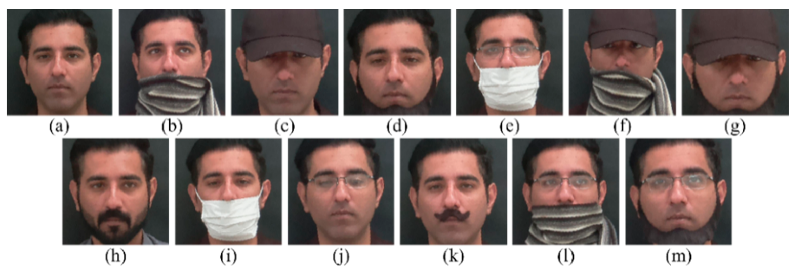
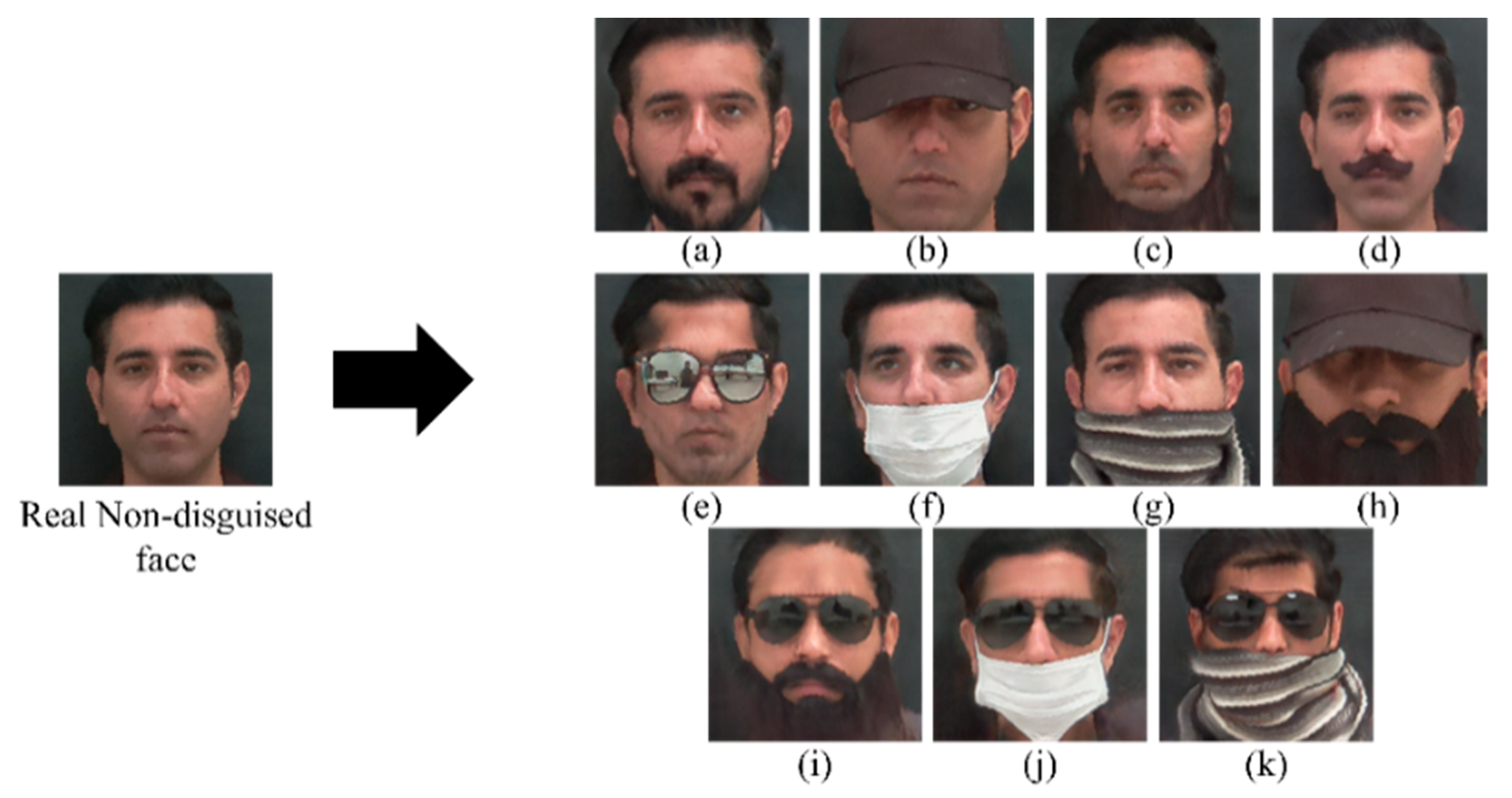
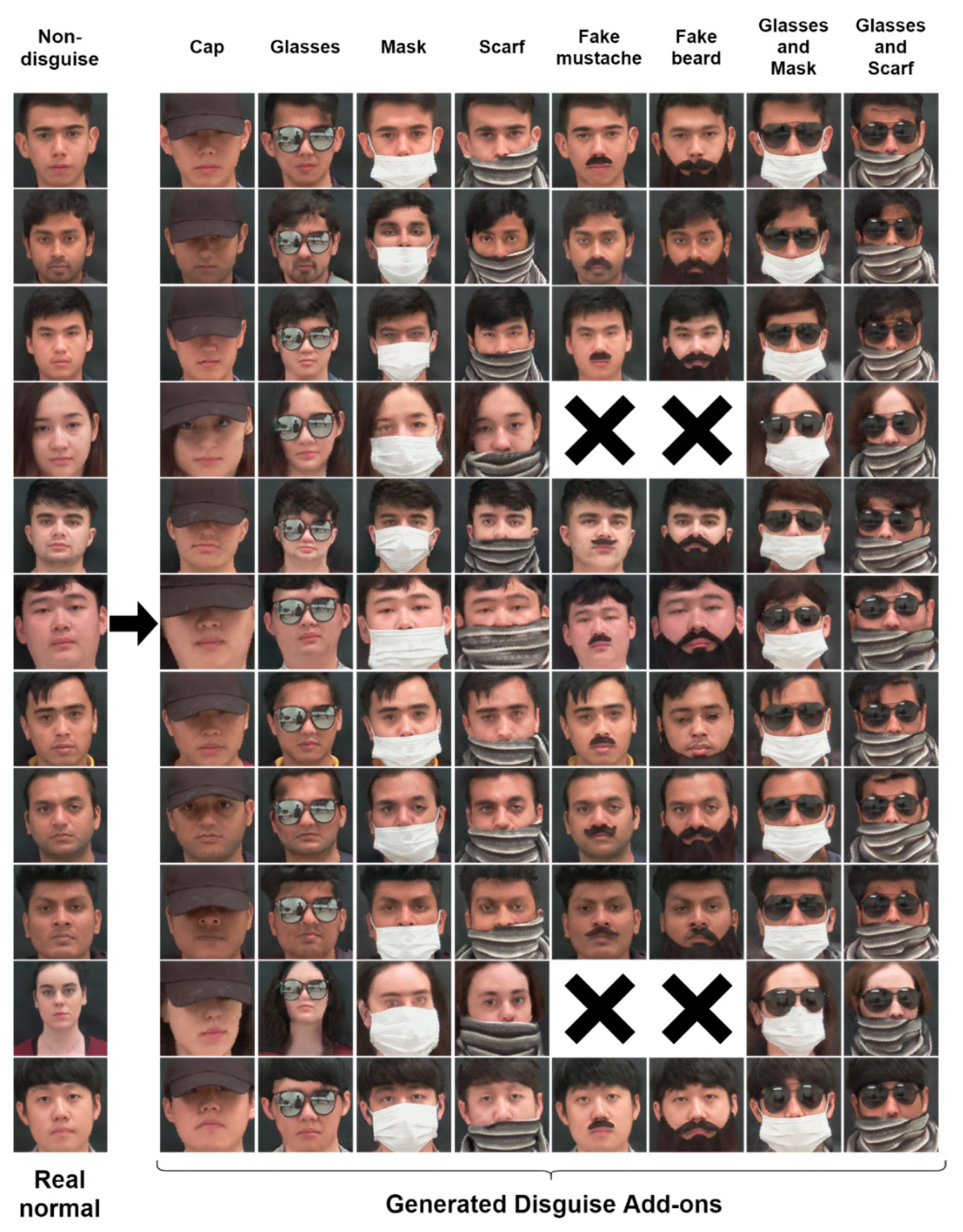
- A synthetic disguised face database, namely, the “Synthetic Disguised Face Database”, is presented as a training and evaluation resource for the robustness of FR algorithms to disguise. The presented DB features facial images with 13 synthetically generated disguise variations;
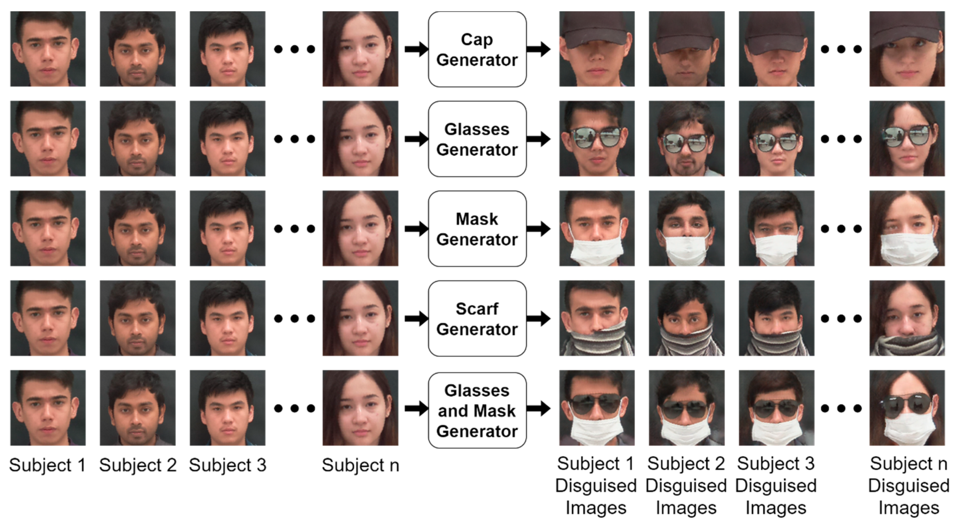
- A methodology employing a GAN and cycle-consistency loss is proposed for synthetic disguised face generation, which will allow future research to extend the existing facial databases. The methodology can be applied to generate disguise add-ons not covered in this study;
- The proposed method can be employed for runtime data augmentation during the training of facial recognition algorithms. Our experimental works prove the value of the proposed methodology over traditional methods of data augmentation;
- A comprehensive analysis is presented by benchmarking the proposed “Synthetic Disguised Face Database” using the state-of-the-art FR method for different experimental configurations. Improved FR performance is achieved using the proposed data on real add-on images;
- An automated filtering scheme is presented that filters out the low-quality image samples from the generated pool of synthetic images. The efficacy of the filtering is shown through the experimental results.
2. Related Work
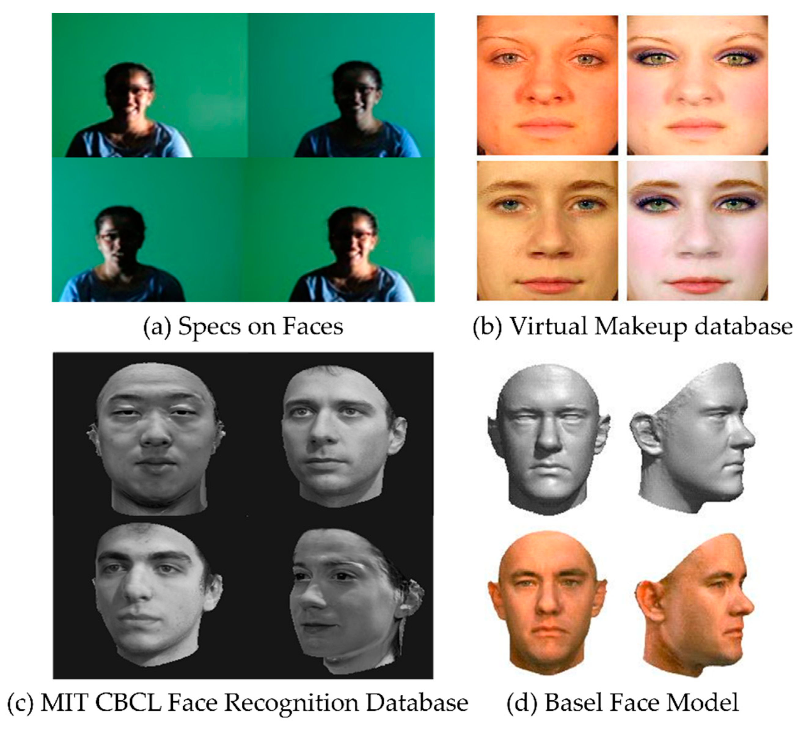
2.1. Face Databases
2.1.1. Databases with Disguised Facial Images
2.1.2. Synthetic Face Databases
2.2. Image Synthesis Based on Generative Adversarial Networks
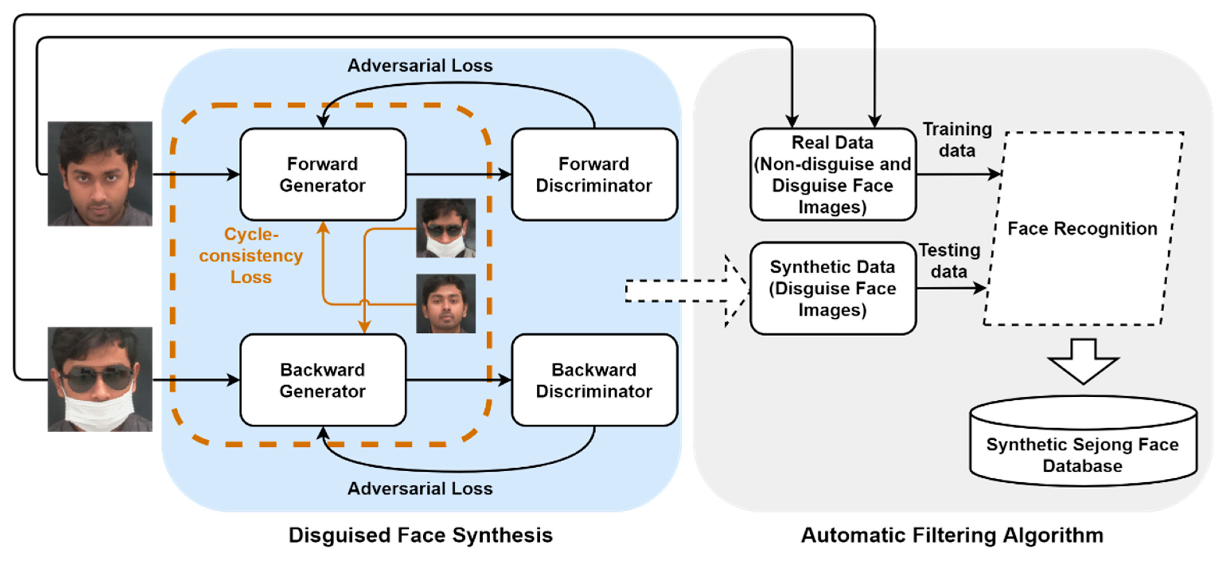
3. Proposed Methodology
3.1. Training the Disguised Face Database
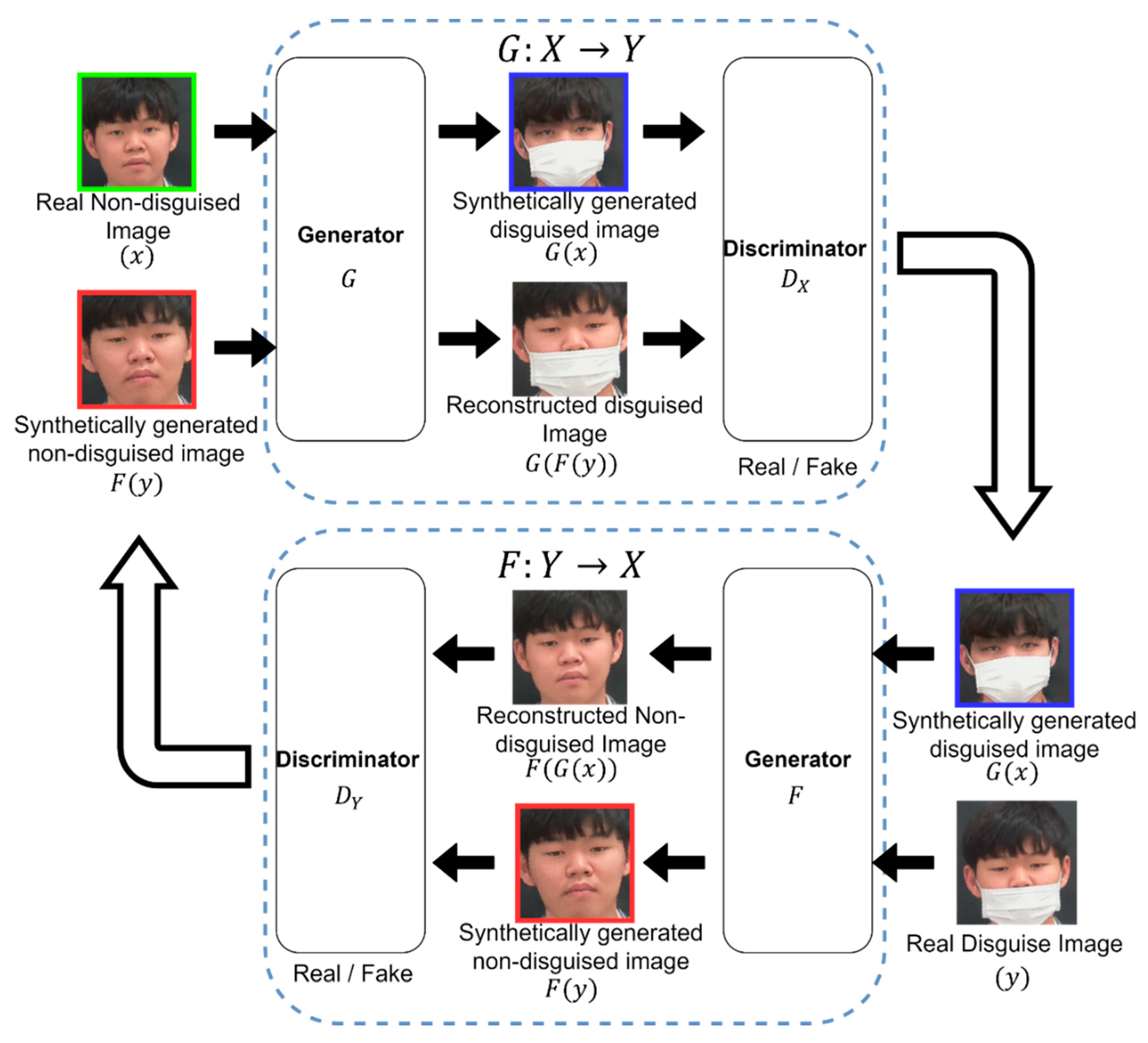
3.2. Disguised Face Synthesis
Convergence Analysis
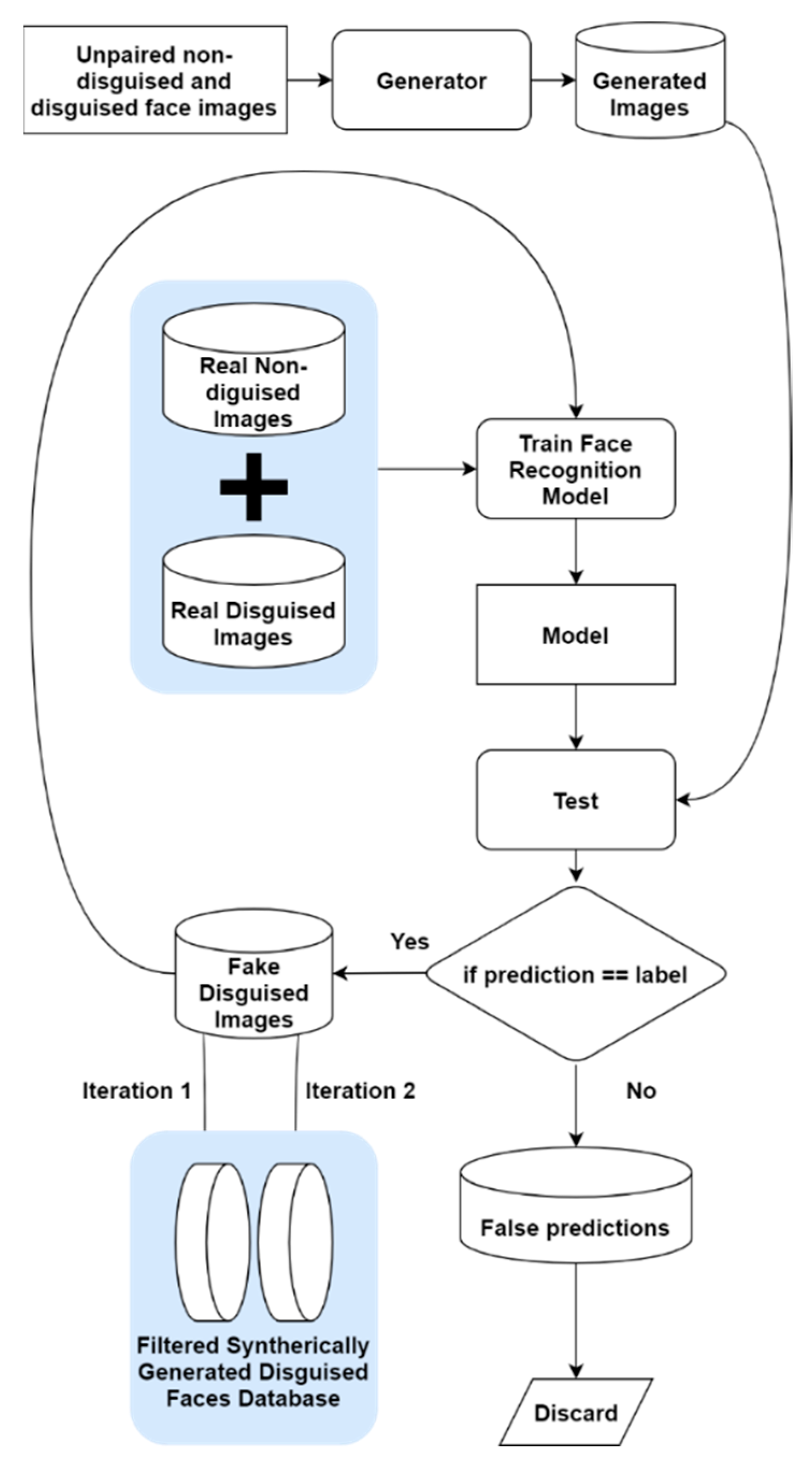
3.3. Automated Filtering Algorithm
4. Experimental Work and Results
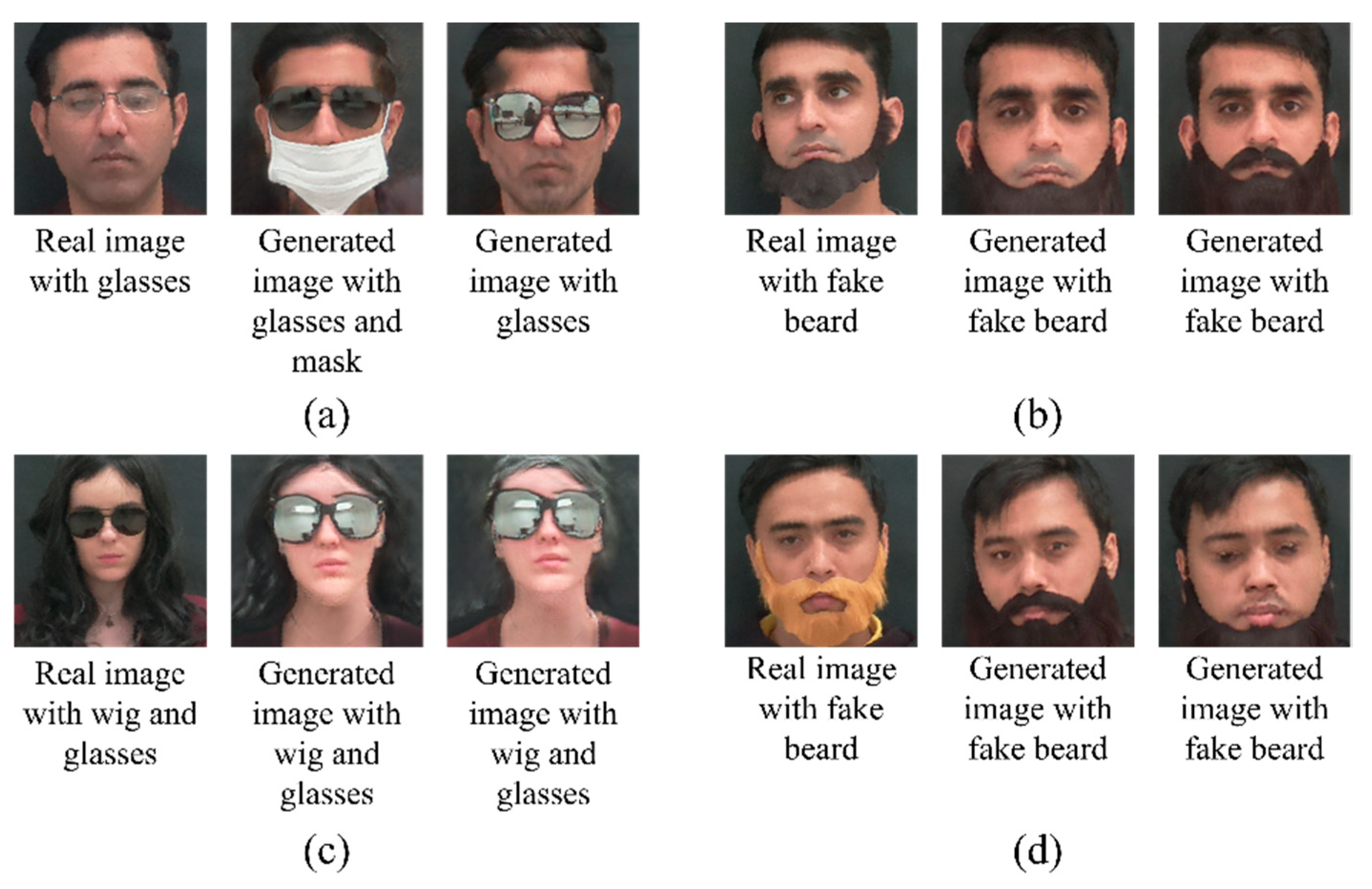
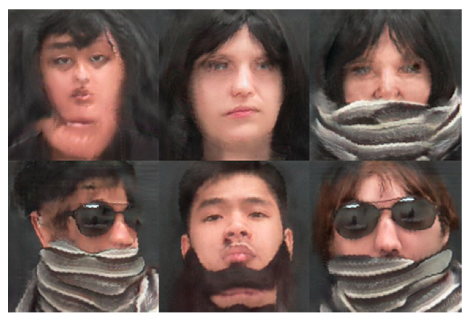
4.1. Disguised Face Synthesis
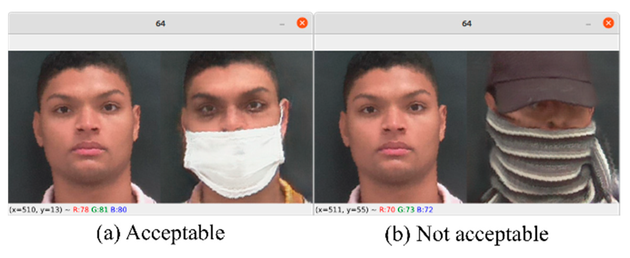
4.2. Manual Filtering
- Both images must be recognizable as the same person;
- The image quality must be lifelike;
- There should be no discrepancy between the original and generated samples, such as in the normalcy of the facial features;
- Ensuring the face is not completely hidden by the generated disguise add-on.
4.3. Automated Filtering Algorithm
| Algorithm 1: Pseudocode of the proposed automated filtering algorithm. |
| 1. Initialization: 2. Real_Normal[] 3. Real_Addons[] 4. Normal_to_Addon_Generator() 5. filtered_Gen_Addons[] 6. false_predictions[] 7. Gen_Addons = Normal_to_Addon_Generator(Real_Normal, Real_Addons) 8. FR_model = SqueezeNet.train(Real_Normal, Real_Addons) 9. predictions[] = FR_model.predict(Gen_Addons) 10. if predictions[x] == ground_truth[x]: 11. filtered_Gen_Addons.append(predictions[x]) 12. else: 13. false_predictions.append(predictions[x]) 14. FR_model_2 = SqueezeNet.train(Real_Normal, Real_Addons+fi ltered_Gen_Addons) 15. predictions[] = FR_model.predict(false_predictions) 16. if predictions[x] == ground_truth[x]: 17. filtered_Gen_Addons.append(predictions[x]) 18. Gen_DB.save(filtered_Gen_Addons) 19. else: 20. false_predictions.append(predictions[x]) 21. false_predictions = Null |
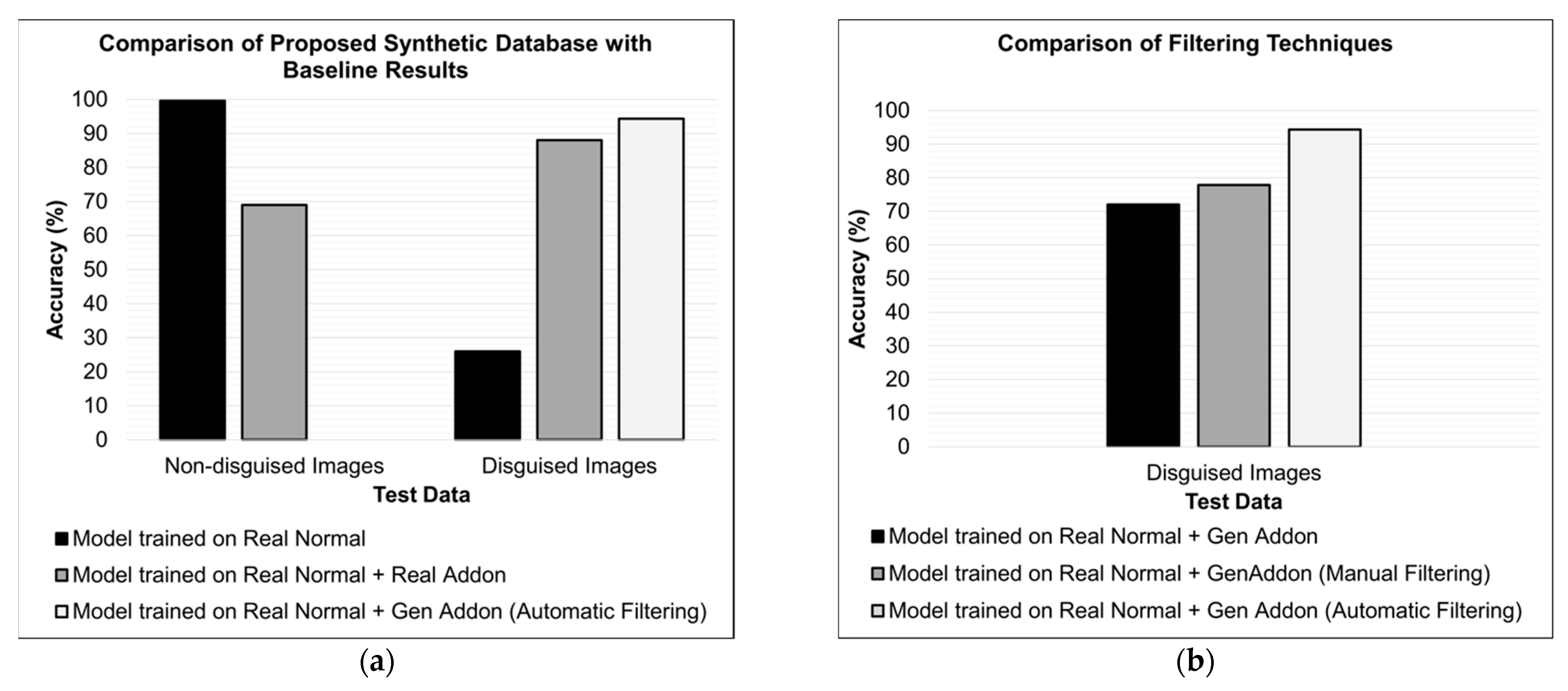
4.4. Facial Recognition Experiments and Results
4.4.1. Experiment Configurations
4.4.2. Facial Recognition Results
5. Discussion
- Human error
- 2.
- The way a model perceives an image is very different than humans
6. Conclusions
Author Contributions
Funding
Institutional Review Board Statement
Informed Consent Statement
Data Availability Statement
Conflicts of Interest
References
- Singh, R.; Vatsa, M.; Bhatt, H.S.; Bharadwaj, S.; Noore, A.; Nooreyezdan, S.S. Plastic Surgery: A New Dimension to Face Recognition. IEEE Trans. Inf. Forensics Secur. 2010, 5, 441–448. [Google Scholar] [CrossRef]
- Phillips, P.J.; Flynn, P.J.; Bowyer, K.W.; Bruegge, R.W.V.; Grother, P.J.; Quinn, G.W.; Pruitt, M. Distinguishing Identical Twins by Face Recognition. In Proceedings of the 2011 IEEE International Conference on Automatic Face & Gesture Recognition (FG), Santa Barbara, CA, USA, 21–25 March 2011; pp. 185–192. [Google Scholar]
- Adjabi, I.; Ouahabi, A.; Benzaoui, A.; Jacques, S. Multi-block Color-binarized Statistical Images for Single-sam-Ple Face Recognition. Sensors 2021, 21, 728. [Google Scholar] [CrossRef] [PubMed]
- Bhatt, H.S.; Bharadwaj, S.; Singh, R.; Vatsa, M. On Matching Sketches with Digital Face Images. In Proceedings of the IEEE 4th International Conference on Biometrics: Theory, Applications and Systems (BTAS), Washington, DC, USA, 27–29 September 2010. [Google Scholar]
- Klare, B.; Li, Z.; Jain, A.K. Matching Forensic Sketches to Mug Shot Photos. IEEE Trans. Pattern Anal. Mach. Intell. 2010, 33, 639–646. [Google Scholar] [CrossRef] [PubMed] [Green Version]
- Chen, X.; Flynn, P.J.; Bowyer, K.W. IR and Visible Light Face Recognition. Comput. Vis. Image Underst. 2005, 99, 332–358. [Google Scholar] [CrossRef]
- Klare, B.; Jain, A.K. HeTerogeneous Face Recognition: Matching NIR to Visible Light Images. In Proceedings of the International Conference on Pattern Recognition, Istanbul, Turkey, 23–26 August 2010. [Google Scholar]
- Singh, R.; Vatsa, M.; Noore, A. Hierarchical Fusion of Multi-Spectral Face Images for Improved Recognition Performance. Inf. Fusion 2008, 9, 200–210. [Google Scholar] [CrossRef]
- Adjabi, I.; Ouahabi, A.; Benzaoui, A.; Taleb-Ahmed, A. Past, Present, and Future of Face Recognition: A Review. Electronics 2020, 9, 1188. [Google Scholar] [CrossRef]
- Taskiran, M.; Kahraman, N.; Erdem, C.E. Face Recognition: Past, Present and Future (a Review). Digit. Signal Process. 2020, 106, 102809. [Google Scholar] [CrossRef]
- Ramanathan, N.; Chellappa, R.; Roy Chowdhury, A.K. Facial Similarity across Age, Disguise, Illumination and Pose. In Proceedings of the International Conference on Image Processing (ICIP), Singapore, 24–27 October 2004; Volume 3. [Google Scholar]
- Singh, R.; Vatsa, M.; Noore, A. Face Recognition with Disguise and Single Gallery Images. Image Vis. Comput. 2009, 27, 245–257. [Google Scholar] [CrossRef]
- Cheema, U.; Moon, S. Sejong Face Database: A Multi-Modal Disguise Face Database. Comput. Vis. Image Underst. 2021, 208–209, 103218. [Google Scholar] [CrossRef]
- Noyes, E.; Parde, C.J.; Colón, Y.I.; Hill, M.Q.; Castillo, C.D.; Jenkins, R.; O’Toole, A.J. Seeing through Disguise: Getting to Know You with a Deep Convolutional Neural Network. Cognition 2021, 211, 104611. [Google Scholar] [CrossRef] [PubMed]
- Dhamecha, T.I.; Nigam, A.; Singh, R.; Vatsa, M. Disguise Detection and Face Recognition in Visible and Thermal Spectrums. In Proceedings of the 2013 International Conference on Biometrics (ICB), Madrid, Spain, 4–7 June 2013. [Google Scholar]
- Min, R.; Kose, N.; Dugelay, J.L. KinectfaceDB: A Kinect Database for Face Recognition. IEEE Trans. Syst. Man Cybern. Syst. 2014, 44, 1534–1548. [Google Scholar] [CrossRef]
- Dhamecha, T.I.; Singh, R.; Vatsa, M.; Kumar, A. Recognizing Disguised Faces: Human and Machine Evaluation. PLoS ONE 2014, 9, e99212. [Google Scholar] [CrossRef] [PubMed] [Green Version]
- Zhang, S.; Liu, A.; Wan, J.; Liang, Y.; Guo, G.; Escalera, S.; Escalante, H.J.; Li, S.Z. CASIA-SURF: A Large-Scale Multi-Modal Benchmark for Face Anti-Spoofing. IEEE Trans. Biom. Behav. Identity Sci. 2020, 2, 182–193. [Google Scholar] [CrossRef] [Green Version]
- Goodfellow, I.; Pouget-Abadie, J.; Mirza, M.; Xu, B.; Warde-Farley, D.; Ozair, S.; Courville, A.; Bengio, Y. Generative Adversarial Networks. Commun. ACM 2020, 63, 139–144. [Google Scholar] [CrossRef]
- Khaldi, Y.; Benzaoui, A. Region of Interest Synthesis Using Image-to-Image Translation for Ear Recognition. In Proceedings of the 2020 4th International Conference on Advanced Aspects of Software Engineering (ICAASE), Constantine, Algeria, 28–30 November 2020. [Google Scholar]
- Khan, A.; Jin, W.; Haider, A.; Rahman, M.; Wang, D. Adversarial Gaussian Denoiser for Multiple-Level Image Denoising. Sensors 2021, 21, 2998. [Google Scholar] [CrossRef] [PubMed]
- Khaldi, Y.; Benzaoui, A. A New Framework for Grayscale Ear Images Recognition Using Generative Adversarial Networks under Unconstrained Conditions. Evol. Syst. 2020, 12, 923–934. [Google Scholar] [CrossRef]
- Zhu, J.-Y.; Park, T.; Isola, P.; Efros, A.A. Unpaired Image-to-Image Translation Using Cycle-Consistent Adversarial Networks. In Proceedings of the IEEE International Conference on Computer Vision, Venice, Italy, 22–29 October 2017; pp. 2242–2251. [Google Scholar]
- Steiner, H.; Kolb, A.; Jung, N. Reliable Face Anti-Spoofing Using Multispectral SWIR Imaging. In Proceedings of the 2016 International Conference on Biometrics (ICB), Halmstad, Sweden, 13–16 June 2016. [Google Scholar] [CrossRef]
- Steiner, H.; Sporrer, S.; Kolb, A.; Jung, N. Design of an Active Multispectral SWIR Camera System for Skin Detection and Face Verification. J. Sens. 2016, 2016, 9682453. [Google Scholar] [CrossRef] [Green Version]
- Raghavendra, R.; Vetrekar, N.; Raja, K.B.; Gad, R.S.; Busch, C. Detecting Disguise Attacks on Multi-Spectral Face Recognition Through Spectral Signatures. In Proceedings of the International Conference on Pattern Recognition, Beijing, China, 20–24 August 2018; pp. 3371–3377. [Google Scholar] [CrossRef]
- Weyrauch, B.; Heisele, B.; Huang, J.; Blanz, V. Component-Based Face Recognition with 3D Morphable Models. In Proceedings of the IEEE Computer Society Conference on Computer Vision and Pattern Recognition Workshops, Washington, DC, USA, 27 June–2 July 2004. [Google Scholar] [CrossRef]
- Paysan, P.; Knothe, R.; Amberg, B.; Romdhani, S.; Vetter, T. A 3D Face Model for Pose and Illumination Invariant Face Recognition. In Proceedings of the 6th IEEE International Conference on Advanced Video and Signal Based Surveillance (AVSS), Genova, Italy, 2–4 September 2009; pp. 296–301. [Google Scholar] [CrossRef]
- Dantcheva, A.; Chen, C.; Ross, A. Can Facial Cosmetics Affect the Matching Accuracy of Face Recognition Systems? In Proceedings of the 2012 IEEE 5th International Conference on Biometrics: Theory, Applications and Systems (BTAS), Arlington, VA, USA, 23–27 September 2012; pp. 391–398. [Google Scholar] [CrossRef] [Green Version]
- Phillips, P.J.; Flynn, P.J.; Scruggs, T.; Bowyer, K.W.; Chang, J.; Hoffman, K.; Marques, J.; Min, J.; Worek, W. Overview of the Face Recognition Grand Challenge. In Proceedings of the 2005 IEEE Computer Society Conference on Computer Vision and Pattern Recognition (CVPR), San Diego, CA, USA, 20–25 June 2005; pp. 947–954. [Google Scholar] [CrossRef]
- Afifi, M.; Abdelhamed, A. AFIF4: Deep Gender Classification Based on AdaBoost-Based Fusion of Isolated Facial Features and Foggy Faces. J. Vis. Commun. Image Represent. 2019, 62, 77–86. [Google Scholar] [CrossRef] [Green Version]
- Isola, P.; Zhu, J.Y.; Zhou, T.; Efros, A.A. Image-to-Image Translation with Conditional Adversarial Networks. In Proceedings of the 30th IEEE Conference on Computer Vision and Pattern Recognition (CVPR), Honolulu, HI, USA, 21–26 July 2017. [Google Scholar]
- Ahmad, M.; Abdullah, M.; Moon, H.; Yoo, S.J.; Han, D. Image Classification Based on Automatic Neural Architecture Search Using Binary Crow Search Algorithm. IEEE Access 2020, 8, 189891–189912. [Google Scholar] [CrossRef]
- Subramanya, A.; Pillai, V.; Pirsiavash, H. Fooling Network Interpretation in Image Classification. In Proceedings of the IEEE International Conference on Computer Vision, Seoul, Korea, 27 October–2 November 2019. [Google Scholar]
- Heusel, M.; Ramsauer, H.; Unterthiner, T.; Nessler, B.; Hochreiter, S. GANs Trained by a Two Time-Scale Update Rule Converge to a Local Nash Equilibrium. In Proceedings of the Advances in Neural Information Processing Systems, Long Beach, CA, USA, 4–9 December 2017. [Google Scholar]
- Salimans, T.; Goodfellow, I.; Zaremba, W.; Cheung, V.; Radford, A.; Chen, X. Improved Techniques for Training GANs. In Proceedings of the Advances in Neural Information Processing Systems, Barcelona, Spain, 5–10 December 2016. [Google Scholar]
- Binkowski, M.; Sutherland, D.J.; Arbel, M.; Gretton, A. Demystifying MMD GANs. In Proceedings of the 6th International Conference on Learning Representations (ICLR), Vancouver, BC, Canada, 30 April–3 May 2018. [Google Scholar]
- Kingma, D.P.; Ba, J.L. Adam: A Method for Stochastic Optimization. In Proceedings of the 3rd International Conference on Learning Representations (ICLR), San Diego, CA, USA, 7–9 May 2015. [Google Scholar]


| Source | Add-On | Abbreviation |
|---|---|---|
| Photographed | No | Real normal |
| Photographed | Yes | Real Disguise |
| Synthetically generated | Yes | Gen. Disguise |
| Database | Total No. of Subjects | Total No. of Images (Visible) | No. of Disguise Images/Subjects (Visible) | Disguise Labels | Gender Male:Female | No. of Add-Ons | Combination Add-Ons |
|---|---|---|---|---|---|---|---|
| I2BVSD [15] | 75 | 681 | 5–9 | ✗ | 60:15 | 5 | ✓ |
| BRSU [24] | 5 | 35 | 4–12 | ✓ | 4:1 | 4–12 | ✓ |
| SDFD [26] | 54 | 285 | 10 | ✓ | 54:0 | 3 | ✓ |
| SFD-A [13] | 30 | 390 | 13 | ✓ | 16:14 | 13 | ✓ |
| SFD-B [13] | 70 | 5250 | 75 | ✓ | 44:26 | 13 | ✓ |
| Proposed Database (Syn-DFD) | 70 | 12,600 | 180 | ✓ | 44:26 | 13 | ✓ |
| Data | FID | KID (Mean ± Standard Deviation) |
|---|---|---|
| Real data splits (baseline) | 30.967 | 0.01128 ± 0.00059 |
| Synthetic Images | 38.177 | 0.01684 ± 0.00037 |
| Add-On | Add-On Name | Number of Images | Gender | ||
|---|---|---|---|---|---|
| Sejong Face Database | Proposed Database | Male | Female | ||
| No Add-on | Natural Face | 15 | - | ✓ | ✓ |
| Real Beard | 10 | 15 | ✓ | ✗ | |
| Accessory Add-on | Cap | 5 | 15 | ✓ | ✓ |
| Scarf | 5 | 15 | ✓ | ✓ | |
| Glasses | 5 | 15 | ✓ | ✓ | |
| Mask | 5 | 15 | ✓ | ✓ | |
| Makeup | 5 | 15 | ✗ | ✓ | |
| Fake Add-on | Wig | 10 | 15 | ✗ | ✓ |
| Fake Beard | 5 | 15 | ✓ | ✗ | |
| Fake Mustache | 5 | 15 | ✓ | ✗ | |
| Combination Add-on | Wig + Glasses | 5 | 15 | ✗ | ✓ |
| Wig + Scarf | 5 | 15 | ✗ | ✓ | |
| Cap + Scarf | 5 | 15 | ✓ | ✓ | |
| Glasses + Scarf | 5 | 15 | ✓ | ✓ | |
| Glasses + Mask | 5 | 15 | ✓ | ✓ | |
| Fake Beard + Cap | 5 | 15 | ✓ | ✗ | |
| Fake Beard + Glasses | 5 | 15 | ✓ | ✗ | |
| Method | Total Number Images | Images/Subjects |
|---|---|---|
| No Filtering | 12,600 | 180 |
| Manual Filtering | 6780 | 88 |
| Automatic filtering | 4158 | 60 |
| Training Configuration | Training Data Type | Total Images | Images per Subject | Subjects | Disguise Add-Ons |
|---|---|---|---|---|---|
| Configuration 0 | Real normal | 685 | 10 | All | All |
| Configuration 1 | Real normal + Real Add-on | 986 | 15 (4 + 11) | ||
| Configuration 2 | Real normal + Gen. Add-on | 1240 | 19 (4 + 15) | ||
| Configuration 3 | Real normal + Real Add-on + Gen. Add-on | 1276 | 20 (4 + 8 + 8) | ||
| Configuration 4 | Gen. Add-on | 1486 | 23 | ||
| Configuration 5 | Real normal + Gen. Add-on (Manual Filtering) | 1240 | 19 (4 + 15) | ||
| Configuration 6 | Real normal + Gen. Add-on (Automatic Filtering) | 1240 | 19 (4 + 15) |
| Test Set | Data Description | Number of Total Images | Number of Images per Subject |
|---|---|---|---|
| Real Normal * | Photographed images of nondisguised faces (reduced set used for Configuration 0) | 251 | 4 |
| Real Normal | Photographed images of nondisguised faces | 564 | 9 |
| Real Add-on | Photographed images of disguised faces | 2272 | 36 |
| Training Configuration | Training Data Type | Accuracy (%) | |
|---|---|---|---|
| Real Normal | Real Add-On | ||
| Configuration 0 | Real normal | 99.6 * | 26 |
| Configuration 1 | Real normal + Real Add-ons | 69 | 88 |
| Configuration 2 | Real normal + Gen. Add-ons | 86 | 72 |
| Configuration 3 | Real normal + Real Add-ons + Gen. Add-ons | 62 | 89 |
| Configuration 4 | Gen. Add-ons | 74 | 71 |
| Configuration 5 | Real normal + Gen. Add-ons w/Manual Filtering | - | 77.8 |
| Configuration 6 | Real normal + Gen. Add-ons w/Automatic Filtering | - | 94.3 |
| Models | Computational Complexity (GMac) | Number of Parameters (Million) | Training | Inference |
|---|---|---|---|---|
| Generator | 56.89 | 11.38 | ✓ | ✓ |
| Generator | 56.89 | 11.38 | ✓ | ✗ |
| Discriminator | 3.15 | 2.76 | ✓ | ✗ |
| Discriminator | 3.15 | 2.76 | ✓ | ✗ |
| Total (Training) | 120.08 | 28.28 | - | - |
| Total (Inference) | 56.89 | 11.38 | - | - |
Publisher’s Note: MDPI stays neutral with regard to jurisdictional claims in published maps and institutional affiliations. |
© 2021 by the authors. Licensee MDPI, Basel, Switzerland. This article is an open access article distributed under the terms and conditions of the Creative Commons Attribution (CC BY) license (https://creativecommons.org/licenses/by/4.0/).
Share and Cite
Ahmad, M.; Cheema, U.; Abdullah, M.; Moon, S.; Han, D. Generating Synthetic Disguised Faces with Cycle-Consistency Loss and an Automated Filtering Algorithm. Mathematics 2022, 10, 4. https://doi.org/10.3390/math10010004
Ahmad M, Cheema U, Abdullah M, Moon S, Han D. Generating Synthetic Disguised Faces with Cycle-Consistency Loss and an Automated Filtering Algorithm. Mathematics. 2022; 10(1):4. https://doi.org/10.3390/math10010004
Chicago/Turabian StyleAhmad, Mobeen, Usman Cheema, Muhammad Abdullah, Seungbin Moon, and Dongil Han. 2022. "Generating Synthetic Disguised Faces with Cycle-Consistency Loss and an Automated Filtering Algorithm" Mathematics 10, no. 1: 4. https://doi.org/10.3390/math10010004
APA StyleAhmad, M., Cheema, U., Abdullah, M., Moon, S., & Han, D. (2022). Generating Synthetic Disguised Faces with Cycle-Consistency Loss and an Automated Filtering Algorithm. Mathematics, 10(1), 4. https://doi.org/10.3390/math10010004