Abstract
This article presents a qualitative mathematical model to simulate the relationship between supplied water and plant growth. A novel aspect of the construction of this phenomenological model is the consideration of a structure of three phases: (1) The soil water availability, (2) the available water inside the plant for its growth, and (3) the plant size or amount of dry matter. From these phases and their interactions, a model based on a three-dimensional nonlinear dynamic system was proposed. The results obtained showed the existence of a single equilibrium point, global and exponentially stable. Additionally, considering the framework of the perturbation theory, this model was perturbed by incorporating irrigation to the available soil water, obtaining some stability results under different assumptions. Later through the control theory, it was demonstrated that the proposed system was controllable. Finally, a numerical simulation of the proposed model was carried out, to depict the soil water content and plant growth dynamic and its agreement with the results of the mathematical analysis. In addition, a specific calibration for field data from an experiment with wheat was considered, and these parameters were then used to test the proposed model, obtaining an error of about 6% in the soil water content estimation.
1. Introduction
A clear example of World Climate Change’s effects has been the generalized increase in drought in some Mediterranean climatic-type areas of South America [1]. Particularly in Chile, since the end of the 1990s, this phenomenon has produced more frequent and severe droughts that have been referred to as a mega-drought [2,3]. Climate change has serious implications for agricultural production [4]. Agriculture is the activity that consumes the most water worldwide because of irrigation, which has been estimated at around 70% [5]. Irrigation is the artificial application of controlled amounts of water to the soil to replace the water consumed by agricultural crops [6]. Irrigation directly affects the plant’s growth, yield, and quality of products, playing a key role in Mediterranean climate-type zones [7]. In Chile, irrigated agriculture represents 52% of the total agricultural surface [8] and 1.7% of the gross domestic product [9], where this economic activity would be impossible without irrigation.
Specific studies have demonstrated the advantages of applying an adequate irrigation strategy [10]. Irrigation scheduling must ideally reflect the crop and climate interactions, considering the water availability, the moment of its application, and the appropriate distribution in the field [6,11,12]. Indeed, several works that analyzed the irrigation strategies used to optimize seasonal water consumption have been developed through engineering crop models, based on biophysical and physiological principles, considering the soil–plant-Atmosphere Continuum (SPAC) system [13,14]. In general, these engineering crop models are computer programs that reliably simulate the growth and development of crops based on specific data. All of them have previously been parameterized and validated, offering reliable results, which have been broadly studied for specific situations [15]. Another alternative to crop modeling is the mathematical approach. Among their advantages are that they enrich the scientific understanding of the phenomena [16] because they manipulate all variables involved, analyzing all the possible responses. To mathematically model how irrigation affects crop growth and the water flow in the SPAC, the phenomenological (or macroscopic) approach is preferred to the mechanistic (or microscopic) one. This is because the phenomenological models are generalist models based on energy and mass transfer principles [17]. Phenomenological models do not require specific soil and plant parameters that may be hard to determine [17,18].
As far as the authors are aware, there are no mathematical models to describe the complete SPAC fluxes. Examples of the effects of the aforementioned mega-drought on agriculture, provided by the development of a generalized mathematical approach, would help to understand water flows in the SPAC. Additionally, these models offer the possibility of analyzing how different irrigation strategies could influence productive parameters such as water productivity, defined as the kilograms of growth per kilogram of water consumed.
We hypothesize that a qualitative mathematical model based on the SPAC interactions will provide reliable trends on the overall relationship among the water in the soil, plant, and growth. Considering that mentioned above, the objective of this work was to develop a phenomenological mathematical model to simulate the relationship between supplied water and plant growth. Taking into account that there are mathematical models that are built to explore, test, and generate hypotheses [19], this tool may provide a useful way of analyzing complex systems and the underlying mechanisms [19,20].
It is important to mention that for simplicity, this model assumes ideal field crop management. Thus, other factors that affect the accumulation of dry matter [21], such as soil nutrients, fertilizers, and so forth were considered ideal, the only limiting factor being the water supply. This model will allow for a description of the effects of different irrigation strategies on crop growth. The main relevance of this study is that it provides a mathematical model in a context in which as far as the authors are aware, there are no similar studies that analyzed the irrigation problem through this approach, coupling between the water supplied to the plant and its dry mass change.
In this work, the development of the model and its analysis is presented as follows. Firstly, we propose a system formulated and studied with an initial available amount of water in the soil. For simplicity, we assumed this concept as being equivalent to the available water capacity (AWC), water holding capacity (SWHC), or total available water (TAW) [6,22]. This initial available amount of water in the soil does not consider external water contributions. This approach is equivalent to assuming, as an initial condition, soil full of water being available for the plant. Additionally, a qualitative analysis of the behavior of the dynamic system was carried out, determining the equilibrium points, the invariant planes, phase diagrams, bounded solutions, and global stability of equilibrium points. Secondly, a system with external water input (i.e., with irrigation) was studied. We started by studying irrigation as a perturbation of the original system, and then it is shown that the said perturbation is a control. Furthermore, simulations were carried out for some parameter values that allowed us to appreciate the dynamics of the system state variables, and then a continuous and periodic irrigation strategy was incorporated to show the effects of irrigation on plant growth. Finally, a calibration and validation example of the resulting parameters of the proposed model will be presented, based on field experiment data obtained from a previous study.
2. Model Formulation
The soil–plant water flow has been traditionally explained by Ohm’s law [23], dividing the water flow into three phases that represent the stages of the system: (1) variation of water at the soil root zone; (2) variation of the water inside the plant; and (3) a third phase that corresponds to the effects of this flow on the variation in the plant growth and size [24]. In this case, the studied phenomenon was irrigation, and how the soil water content variations affect the growth of plants. This process is represented by the following abstraction: The process begins by considering that the soil at the root-zone of the plant acts like a pond that contains the available water for plant water consumption . Then the water from the soil fluxes through the plant to the atmosphere, and due to photosynthesis, a proportion of that water is transformed into biomass.The other proportion remains in the plant cells, and a fraction of it allows their growth [25]. The latter has traditionally been assumed as a sigmoidal growing shape. Under these assumptions, a three-phase model is proposed: (1) Soil water availability , (2) water inside the plant available for its growth , and (3) the plant size or amount of dry matter .
2.1. Water Dynamics at the Root Zone
In the development of this model, the soil at the root zone was assumed to act as a pond. This assumption is of an analogy that will be repeatedly used in the text. At the beginning of the growing cycle, it is assumed that this pond starts at full capacity of water . Then, during the growing cycle, the variations of the water in the pond are composed of two terms: the first is proportional to the amount of water in the soil at the root-zone, and the second term accounts for the interaction of water inside the plant with the water of the pond. Here, it must be considered that for large values , the rate reaches a constant threshold, as follows:
where r is a constant that modifies the limiting factor of the water inside the plant, is the internal rate of decline in pond water by evaporation, and is the intrinsic rate of water that goes to the plant.
2.2. Water Dynamics Inside the Plant
The water flow from the soil to roots and then to the whole plant is considered as a mass transfer process, where the water that enters the plant is equal to that lost through transpiration, plus that which is stored in the tissues. Then the variation of water inside the plant available for its growth, responds to the type,
Water absorption: The plant absorbs the soil-water in proportion to the amount of water that the pond has in interaction with the water inside the plant ; however, the water inside the plant for large values reaches a constant rate,
with being the intrinsic rate of increase of the water inside the plant.
Water removed: The water that passes throughout the plant is moved by transpiration, which is considered proportional to the amount of water that the plant has, and the other is retained in the plant tissues and a fraction of it is utilized for plant growth. This process is considered proportional to the gain of mass (this term gain will be defined later) in interaction with the amount of water . Then:
with constant being the rate of decrease of water inside the plant, and is the plant growth rate.
2.3. Plant Growth Dynamics
For the growth of the plant, the variation of dry matter is considered, and it is the result of a gain less than a degradation term, where an alternative that includes the Ref. [24] is,
where represents the amount of dry mass at time t, the constant corresponds to the intrinsic growth rate of the plant, g modifies the limiting factor of plant growth, m corresponds to the rate of degradation of the plant, and factor n allows for modification of the rapidity of growth of the plant.
Let us now discuss the first term of the Equation (6), as in any population, particularly of cells of a plant, the rate of gain of a new mass per unit of time at all times t can be a function of important internal or environmental parameters, also of the same accumulated mass as a limiting element to growth (dense dependence with negative correlation). The form of the function that represents the gain and that corresponds to the first term of (6) is , which can be seen to be very sensitive to the parameter n. The form of G (x) is discussed below for some intervals of n, with constant .
Next are four cases for different values of n:
- (a)
- If , then , which for tends to , which is not realistic, because the dry mass can not grow forever.
- (b)
- For , it has , and the dry mass gain increases linearly with the size of the plant, which, like the previous case, does not represent reality.
- (c)
- For , if then , it tends quickly to zero. This case is unusual, and has been discarded in further analysis.
- (d)
- Finally, the fourth case, with , was assumed for the model.
Figure 1 illustrates the effects of parameter n on the function that represents the mass gain. Five different values of n are taken into account, considering the four previous cases.
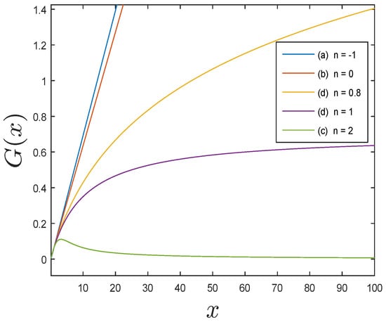
Figure 1.
Rate of mass gain as a function of size of the plant, considering the following parameter values: and . This figure shows that for values of (blue, red; cases (a), and (b)), the gain in dry matter grows rapidly (monotonous growth). Similarly, for (green; case (c)), the dry matter gain falls very quickly to zero. For values of (yellow, case (d)) and (purple; case (d)) the behavior of the gain is more realistic. In this work, a value of was assumed for the model.
In relation to the second term of Equation (6), the literature assumes that the plant in any state of growth has some loss of mass at time t, considered proportional to the size of the plant at time , with a constant degradation rate m.
Figure 2 represents the size of the plant as a function of time, obtained from the relationship (6). It can be seen in Figure 2 that at the beginning of the time scale, the size of the plant tends to grow unlimitedly in a short time interval, for values of (blue, red). This situation does not agree with plants which grow in a common pattern. In nature, plants can present with accelerated growth in their first growth stages, but it then decreases in their maturity until reaching a plateau; after that, there is a decrease in their harvest, or after the end of each growing season [22]. For n = 2 (green), the plant’s size reaches a constant value very soon (there is no growth), which is not adjusted to the aforementioned pattern of plant growth. By assuming values of (yellow) and (purple), the simulated behavior of the size of the plant over time shows a shape that reflects the natural plant growth pattern.
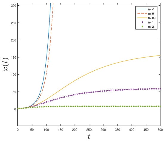
Figure 2.
Simulation of dry mass growth as a function of time, where: n is the factor that allows for modification of the plant’s rapidity of growth in t time (days), and is the amount of dry matter (unit of mass). For parameter values , , and .
Finally, in the first term of Equation (6), the intrinsic growth rate of the plant is considered a function of omega, , to incorporate an interaction with the water entering the plant, where is a proportionality constant that accounts for the influence of water inside the plant on the growth of the crop. In this way, the gain increases when more water enters the plant, then Equation (6) remains:
where one should remember that , and for simplicity, we chose .
Assumptions
- A1: In relation to the water that flows from the pond to the plant, it is assumed that the water absorption rate of the plant is less than or equal to the rate of loss of water from the pond to the plant, that is, .
- A2: In relation to the process of photosynthesis and plant growth, it is assumed that the dry matter accumulation rate of the plant is approximately equal to the rate of decrease of the water inside the plant that goes to photosynthesis. This assumption is supported by the equation of photosynthesis [26]. Photosynthesis is the process that occurs in plants (chlorophyll) where the solar energy, through the water hydrolysis, is used for atmospheric carbon dioxide assimilation, resulting in the production of carbohydrate molecules and oxygen. The balanced general equation of this phenomenon, for C3 plants, is as follows: , resulting in .
- A3: It is assumed that the rate of water loss through transpiration is greater than the rate of water loss through evaporation , which is . In addition, it is assumed that the degradation rate of the plant m is greater than the rate of water loss through evaporation , which is . Finally, it is assumed that
2.4. Mathematical Model
From Equations (1)–(7), the following dynamic system is obtained, which represents the coupling between the water supplied to the plant and the change of its dry mass.
More simply,
where represents the right side of the system (8).
For obtaining a system of nonlinear differential equations in three dimensions where it has been used, is a constant that represents the intrinsic rate of water decrease by photosynthesis. The parameters are presented in Table 1.

Table 1.
Parameters considered in the present study.
System (8) is defined in the region .
Remarks
- Plant size variation. In the Equation (8), the first term of corresponds to the growth rate of the plant due to the water inside the plant represented by , and the expression is the limiting factor of plant growth. The second term corresponds to the rate of degradation of the plant.
- Variation of water inside the plant. The first term of accounts for the rate of increase of the water inside the plant due to the water coming from the pond v, and the expression corresponds to the limiting factor of the increase in water inside the plant. The second term represents the rate of decrease of the water inside the plant caused by transpiration. The third term is the rate of water loss inside the plant as a result of photosynthesis, and the expression represents the rate of decrease per capita, the value corresponds to half of the maximum decrease rate .
- Variation of water in the pond. The first term corresponds to the rate of decrease in pond water due to evaporation losses. The second term is the rate of decrease of the pond water flowing into the plant, the expression represents the rate of decrease per capita of pond water flowing to the plant, and the value corresponds to half of the maximum decrease rate .
3. Main Results
Lemma 1.
The coordinate planes of the system (8) are invariant.
Proof.
It will be proved that the plane is invariant, and the proof is similar for the other planes. On one side, let be the plane with , then the vector is always normal to . On the other hand, points of comply, .
In this way, the following result is obtained:
which shows that the plane is invariant. □
Proposition 1.
The solutions of system (8) are uniformly bounded.
Proof.
Defining as:
Then,
and by assumption A3, the . Then, satisfies
□
The equilibrium points of the system (8) are:
. Considering that the state variables represent non-negative quantities, then only the equilibrium points that are in the first octant are of interest. Thus, the only equilibrium point of interest is .
Lemma 2.
The equilibrium point is locally asymptotically stable.
Proof.
The eigenvalues of the Jacobian matrix evaluated at the point are: ; therefore, is locally stable. □
Proposition 2.
is a globally exponentially stable equilibrium point.
Proof.
Using the direct method of Lyapunov demonstrates the global exponential stability of the system. The following scalar function is considered:
- (i)
- Clearly, and for .
- (ii)
- .Then, in , given that all the parameters: and are positive, and the state variables are also positive.
- (iii)
- . With , according to the Assumptions , obtaining .On the other hand, , with , according to the Assumptions , obtaining .Obtaining .
- (iv)
- , according to the Assumptions,.Obtaining .
- (v)
- Since the Lyapunov function it is strictly increasing, .
□
4. Modeling with Irrigation
To consider adding external water to the system, in Equation (9), a term is incorporated that accounts for the way in which the water is added.
The term is considered a perturbation of the system. Suppose the perturbation term satisfies the linear growth bound.
where is a nonnegative constant,
where and are defined by the Lyapunov function (11) of the nominal system (9) that satisfies the following three conditions,
where , ,
, .
Considering the Assumptions of the model, the following is obtained: , , . For the case , from the Assumptions A2, we have that , where from A1 you get , then , obtaining ; then, we assume that
Lemma 3.
Suppose the perturbation term satisfies , for . Then, equilibrium point is globally exponentially stable of the system (12).
Proof.
Now we are going to consider the more general case , and we cannot expect the solutions to approach the origin for long times, but we can ensure that the solutions are ultimately confined by a small bound in some sense.
Theorem 1.
5. Irrigation as Control
Now the external water added to the system is considered as a control , and from (9) the equation of state is obtained, with Thus, the system (12) assumes the following form:
with output equation
Lemma 4.
Proof.
We define , then . Thus,
and is obtained. Finally,
Therefore,
In the second case, we calculate the rank of matrix constructed from Lie brackets, and check that the distribution is involutive.
- (I)
- Let’s evaluate the second term of ,Now let’s calculate the third term of :The matrix remainsThen
- (II)
- The distribution is involutive, since:
- (i)
- Clearly, is linearly independent, with and
- (ii)
- Let’s evaluate the range of ..
□
Corollary 1.
6. Numerical Examples and Simulations
6.1. Dynamics of the State Variables of the System
The model (9) was implemented using a script written using Matlab© R2019a (Mathworks Inc., Natick, MA, USA). It is important to highlight that water is the main component of plants—approximately between 80 % and 90 % of the fresh weight in herbaceous plants, and more than 50 % in woody plants [23]. In this simulation, it has been considered for the initial values of the states that 70% corresponds to water inside the plant available for growth, and 30% corresponds to dry mass, then , and (Figure 3, Figure 4 and Figure 5). The parameter was taken from Thornley [24]. The parameters and were conditioned by Assumption A3, and , and we took , and and . From Assumption A2, . Parameters , and r were arbitrarily manipulated to fit the curves, and do not necessarily represent values associated with particular cases, with the condition imposed by Assumption A1, .
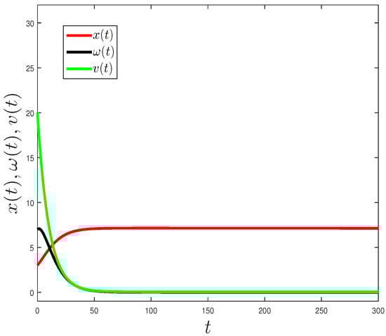
Figure 3.
State dynamics for the system without irrigation, time t in days, where (green line), (black line), and (red line) are the water available in the soil, the water inside the plant, and the amount of dry matter, respectively. Parameter values: , , , , , , , , , .
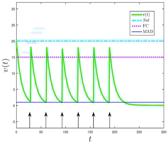
Figure 4.
Soil water content for the plants’ growth. The horizontal lines represent the soil water thresholds, Saturated soils (Sat, upper line), Field Capacity (FC), and Management Allowed Depletion (MAD, bottom line). The vertical arrows indicate the times when irrigation is applied. Initial conditions , parameter values , , , , , , , , .
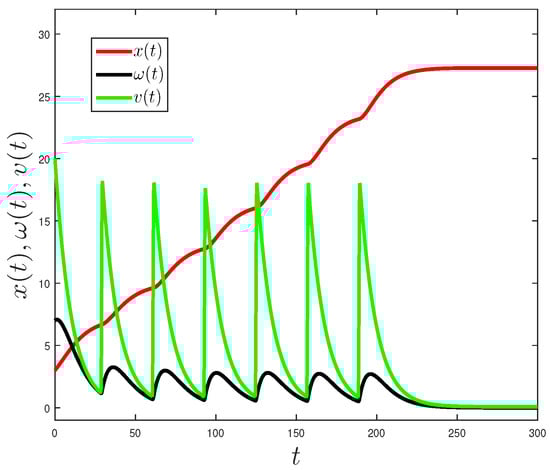
Figure 5.
State dynamics for the system with irrigation, time t in days, where (green line), (black line), and (red line) are the water available in the soil, the water inside the plant, and the amount of dry matter, respectively. Parameter values: , , , , , , , , , .
Figure 3 presents a simulation of the system without irrigation, which allows us to appreciate the dynamics of the states, for a cultivation period of 300 days. It can be seen that the curve that represents the water available in the soil (green line) approaches zero for a time t around 35, like the water available inside the plant (black line). Additionally, the amount of dry matter (red line) has strong growth of t around 30, and then very slowly decays.
The study of the behavior of the long-term solutions and their stability was carried out in order to determine the validity of the model and its construction in qualitative terms, however, for practical application purposes, the behavior of the crops in the short term is of interest for decision-making. This motivated the next numerical scenario.
6.2. Irrigation Strategy
Now we incorporate irrigation in the system (9) to analyze through simulations how irrigation of a farm field influences plant growth. For this, an irrigation function is incorporated to state variable of the system (9). We consider a bounded, continuous, differentiable, and periodic irrigation function, Figure 6. Crop seasons were of 300 days, with irrigation during the first 200 days, an irrigation period of 32 days, with each watering lasting one day, and levels of irrigation of 30 volume units.
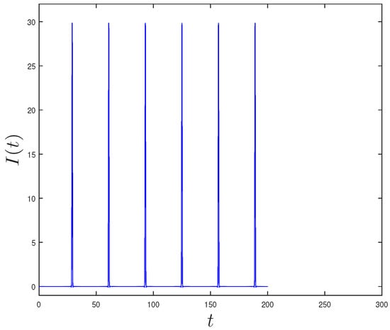
Figure 6.
Irrigation function in days t. This function is considered bounded, continuous, differentiable, and periodic in order to represent a realistic case. Six watering applications were considered during the season.
When applying the irrigation function to the system (9), there are fluctuations in the amount of water in the soil available for the growth of the plant, as shown in Figure 4. The horizontal lines mark the thresholds for the availability of water in the soil; most of the pores of Saturated soils (Sat) were occupied by water, which prevents the uptake of oxygen by the roots; Field Capacity (FC) is the amount of water in the soil after drainage; and Management Allowed Depletion (MAD) is the percentage of depletion without reduction of crop yield [6]. The vertical arrows indicate the times when irrigation is applied. Six irrigation applications were made during the season, where the first irrigation was carried out when the initial amount of water reached the MAD value, approximately at ; thus, the irrigation period will be 32. The amount of water supplied in each irrigation slightly exceeds FC.
Figure 5 shows the dynamics of the states of system (9) when applying the irrigation function of Figure 6. Comparing Figure 5 with Figure 3, it is possible to see how irrigation affects crop growth. The irrigation schedule allows the accumulation of dry matter x(t) to increase during the irrigation period (200 days in the numerical example). When irrigation is suspended, and tend to zero, and the process of dry matter accumulation stops.
6.3. Assessment of the Model Performance Using Experimental Data
As our work did not have its own field data, and under the need to evaluate the performance of the proposed model, it was assessed against field data obtained from Andarzian et al. [28]. In this work, the authors presented the results from a field experiment carried out on full and deficit irrigated wheat production in Iran. Mainly, data from this research were obtained from [28] (Figure 1, page 4), which describes the soil moisture dynamics for wheat (1) under full and (2) with water deficit irrigation. The values from this figure were hand-extracted to a Comma Separated Values (CSV) file, using the WebPlotDigitizer webpage (https://automeris.io/WebPlotDigitizer/, accessed on 13 December 2021). Please consult the work of Andarzian et al. [28] for more details.
Data-processing and statistical analysis. The system (9) was solved numerically, adjusting the output for the soil water content, considering the case under water deficit. This parameterization was carried out using a nonlinear least squares curve-fitting method [29], by occupying a script developed in Matlab© R2019a (Mathworks Inc., Natick, MA, USA). The actual data from the soil moisture obtained from Andarzian et al. [28] were used to fit the parameters to find the best solution. The resulting parameter values of the model that minimized the difference between simulated and measured data are presented in Table 2. The performance of the data fit is presented in Figure 7.
Table 2.
Proposed model resulting parameters.
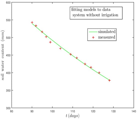
Figure 7.
Model fit from the deficit irrigated wheat data (data extracted from Andarzian et al., [28].)
Then the parameters from Table 2 were used to test the proposed model, considering the simulation with irrigation . For this purpose, the data extracted from Andarzian et al. [28] for the experiment with full irrigation were used as ground truth, and they were compared against the proposed model’s outputs. The model performance of that simulated against measured data was carried on by the classical curve fit suggested by Mayer and Butler [30]. The statistical parameters used were the Pearson’s correlation coefficient (r), the Mean Absolute Error (MAE), and the Root Mean Square Error (RMSE) deviance parameters. Figure 8 shows the graphs of the simulated and measured data.
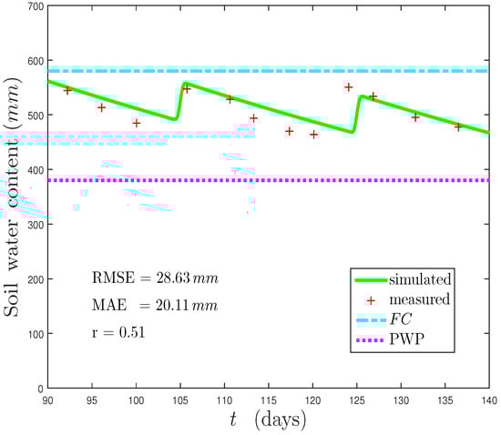
Figure 8.
Soil water content trends for modeled and actual data for full irrigated wheat (using the calibrated parameters from Table 2, and measured data from Andarzian et al. [28]). Field Capacity (FC), Permanent Wilting Point (PWP), Root Mean Square Error (RMSE), Mean Absolute Error (MAE), and Pearson’s correlation coefficient (r).
The performance of the modeled against measured values, depicted in Figure 8, showed good trends, highlighting the model’s capabilities to simulate the soil water content behavior. The green line was very close to the measured values (orange crosses), considering a cycle of two irrigations for the experiment on wheat. Regarding the statistical validation, the r = 0.51, with an RMSE and MAE of 28.63 and 20.11 mm, can be considered acceptable for irrigation purposes [28,31,32].
7. Discussion
As far as the authors are aware, in the literature, there is a large number of works that study the irrigation phenomenon considering the SPAC system from computational simulations [6,15,20,33,34,35,36]. The models above have been described as methods to understand and reproduce the water fluxes from the root zone to the atmosphere, evaluating specific climatic scenarios and their influence on plant growth. These approaches can be used to simulate point examples, and are very useful for particular field conditions and management. In our case, the qualitative characteristics of the proposed model could allow for simulations of all situations. In the development of this model, it was assumed that the relation between irrigation and plant growth could be compartmentalized into three parts: The soil water availability, (2) the available water inside the plant for its growth, and (3) the plant size or amount of dry matter. In the construction of the model, it has been considered that the water in the soil only reduces due to the evaporation from the soil and the water consumed by the plant by the transpiration. This last flux allows the plant to photosynthesize. This phenomenon increases the plant’s biomass (dry mass amount) due to the water inside the plant available for growth, considering the losses due to degradation. For the relationship between the parameters of the model (8), whose description is given in Table 1, some assumptions have been considered: the rate of flow of water from the pond (soil) to the plant () being greater or equal to the rate of flow of water entering from the soil to the plant (). Furthermore, the rate of accumulation of dry matter (or dry mass) () is approximately equal to the rate of decrease of the water inside the plant that goes towards photosynthesis (k). Finally, the rate of flow of water corresponding to transpiration () is greater than the flow rate of evaporated water ().
The stability analysis of the proposed model was divided into two parts, with and without an external water supply. The system without an external water supply was first studied (8). Second, it was studied with an external water supply giving rise to the two models (12) and (23) based on the perturbation theory and control theory results.
For the analysis of the model, it was considered that the soil starts with a certain amount of water, the plant starts with a certain size, and at the beginning of the process, there is a certain amount of water inside the plant available for growth. These considerations were both for the system without external water supply (or irrigation) (8) and also for the systems with an external water supply, both the perturbed (12) and control (23).
The proposed mathematical model (8) without an external water supply meets the following properties: The solutions of the system are uniformly bounded, and this indicates that the states’ variables do not grow indefinitely. It was also found that the system has a single equilibrium point given by (0,0,0) which is globally exponentially stable, showing that given any initial condition, the water–plant interaction does not persist in the long term.
The simulation shown in Figure 3 indicates that the proposed mathematical model allows to qualitatively account for the expected behavior in the dry matter changes of the plant as a function of the soil water, and the dynamics of the curves are in accordance with what is expected in general for the behavior of plants.
The effect of an external water supply was subsequently studied. In the first place, the external water supply was treated as a perturbation to the original model (8) through an irrigation function, obtaining the system (12). If the perturbation is bounded and null at the origin, that is, at the beginning of the process, there is no external water supply, then the equilibrium point (0,0,0) is globally exponentially stable, maintaining the stability behavior similar to the original system. If the perturbation is not null at the origin, that is, at the beginning of the process there is an external water supply, a bound was found in terms of the system parameters so that said perturbation maintains similar stability to the original system, this bound turned out to be proportional to inner rate of decrease of the soil water content (). Second, the irrigation was treated as a control (23) and it was found that the system is controllable by taking the size of the plant as the output state, which implies that it is theoretically possible to achieve a desired plant size level from any initial state through a continuous irrigation strategy dependent on the state variables.
Figure 4 and Figure 5 show that when applying continuous and periodic irrigation, there are fluctuations in the amount of water in the soil available for the plant, that oscillate between the thresholds for the availability of water in the soil FC and MAD, thus achieving sustained growth of the plant. This was most evident when comparing Figure 3 and Figure 5.
After the parameterization, the proposed model obtained an acceptable simulation of the soil water content seasonal trends (Figure 8), considering a specific calibration for field data, from an experiment on wheat. Notwithstanding, this is a specific example. The proposed model’s performance should be parameterized and validated whenever tested against field data.
8. Conclusions
In this work, a mathematical model based on the SPAC system was proposed from a phenomenological paradigm to study the effect of irrigation on plant growth from a macroscopic perspective. This mathematical approach has been focused on increasing the understanding of plant–water relation growth dynamics from a qualitative point of view.
A contribution of this work is that it provides a mathematical simplified model to describe the dynamic of the water from the root zone to the plant, their interactions, and how they affect plant growth. This is the first attempt to approximate such a phenomenon in a simple way.
The application of the model to actual data resulted in an acceptable performance for wheat irrigation, considering specific parameters calibration. For future work, it is expected to adjust the model with the results of other field experiments quantitatively. Their potential for use and limitations will depend on its configuration and calibration using ground truth data. Its simplicity, if adequately parameterized, could lead to obtaining representative simulations for more specific purposes, such as irrigation management. As indicated herein, the complex interactions among the soil water availability, water availability, and plant growth open new needs for exploring an adjustment to the proposed model.
Author Contributions
V.D.-G., A.R.-P. and M.C.-B., conceived this research. V.D.-G. and A.R.-P., contributed to the mathematical model development and analyses. All authors worked extensively in the preparation of the whole manuscript, the results interpretation and their discussions. All subsequent revisions were done in the same way. All authors have read and agreed to the published version of the manuscript.
Funding
This study was partially supported by the Doctorate Scholarship of the Universidad Católica del Maule, and the Chilean government through the Agencia Nacional de Investigación y Desarrollo (ANID), throughout the “Programa FONDECYT Iniciación en la Investigación, año 2017” (grant No. 11170323).
Institutional Review Board Statement
Not applicable.
Informed Consent Statement
Not applicable.
Data Availability Statement
Not applicable.
Conflicts of Interest
The authors declare no conflict of interest.
References
- Prudhomme, C.; Giuntoli, I.; Robinson, E.L.; Clark, D.B.; Arnell, N.W.; Dankers, R.; Fekete, B.M.; Franssen, W.; Gerten, D.; Gosling, S.N.; et al. Hydrological droughts in the 21st century, hotspots and uncertainties from a global multimodel ensemble experiment. Proc. Natl. Acad. Sci. USA 2014, 111, 3262–3267. [Google Scholar] [CrossRef] [Green Version]
- Aldunce, P.; Araya, D.; Sapiain, R.; Ramos, I.; Lillo, G.; Urquiza, A.; Garreaud, R. Local perception of drought impacts in a changing climate: The mega-drought in central Chile. Sustainability 2017, 9, 2053. [Google Scholar] [CrossRef] [Green Version]
- Duque-Marín, E.; Rojas-Palma, A.; Carrasco-Benavides, M. Mathematical modeling of fruit trees’ growth under scarce watering. J. Phys. Conf. Ser. 2021, 2046, 012017. [Google Scholar] [CrossRef]
- Rosegrant, M.W.; Ringler, C.; Zhu, T. Water for agriculture: Maintaining food security under growing scarcity. Annu. Rev. Environ. Resour. 2009, 34, 205–222. [Google Scholar] [CrossRef]
- FAO. AQUASTAT Main Database-Food and Agriculture Organization of the United Nations (FAO); FAO: Rome, Italy, 2015. [Google Scholar]
- Waller, P.; Yitayew, M. Irrigation and Drainage Engineering; Springer: Berlin/Heidelberg, Germany, 2015. [Google Scholar]
- Romero, M.; Luo, Y.; Su, B.; Fuentes, S. Vineyard Water Status Estimation Using Multispectral Imagery from an UAV Platform and Machine Learning Algorithms for Irrigation Scheduling Management. Comput. Electron. Agric. 2018, 147, 109–117. [Google Scholar] [CrossRef]
- ODEPA. Chilean Agriculture Overview 2017. Available online: https://www.odepa.gob.cl/wp-content/uploads/2017/12/panoramaFinal20102017Web.pdf (accessed on 3 March 2021).
- ODEPA. Chilean Agriculture Overview 2018. Available online: https://www.odepa.gob.cl/wp-content/uploads/2018/01/ReflexDesaf{_}2030-1.pdf (accessed on 3 March 2021).
- Kharrou, M.H.; Er-Raki, S.; Chehbouni, A.; Duchemin, B.; Simonneaux, V.; LePage, M.; Ouzine, L.; Jarlan, L. Water use efficiency and yield of winter wheat under different irrigation regimes in a semi-arid region. Agric. Sci. China 2011, 2, 273–282. [Google Scholar] [CrossRef] [Green Version]
- Pereira, L.S. Water, agriculture and food: Challenges and issues. Water Resour. Manag. 2017, 31, 2985–2999. [Google Scholar] [CrossRef]
- Gurovich, L.A.; Riveros, L.F. Agronomic operation and maintenance of field irrigation systems. In Irrigation-Water Productivity and Operation, Sustainability and Climate Change; IntechOpen: London, UK, 2019; p. 84997. [Google Scholar] [CrossRef] [Green Version]
- Belaqziz, S.; Mangiarotti, S.; Le Page, M.; Khabba, S.; Er-Raki, S.; Agouti, T.; Drapeau, L.; Kharrou, M.; El Adnani, M.; Jarlan, L. Irrigation scheduling of a classical gravity network based on the Covariance Matrix Adaptation—Evolutionary Strategy algorithm. Comput. Electron. Agric. 2014, 102, 64–72. [Google Scholar] [CrossRef] [Green Version]
- Bonan, G.; Williams, M.; Fisher, R.; Oleson, K. Modeling stomatal conductance in the earth system: Linking leaf water-use efficiency and water transport along the soil–plant–atmosphere continuum. Geosci. Model Dev. 2014, 7, 2193–2222. [Google Scholar] [CrossRef] [Green Version]
- Oteng-Darko, P.; Yeboah, S.; Addy, S.; Amponsah, S.; Danquah, E.O. Crop modeling: A tool for agricultural research—A. J. Agric. Res. Dev. 2013, 2, 001–006. [Google Scholar]
- Roose, T.; Schnepf, A. Mathematical models of plant–soil interaction. Philos. Trans. R. Soc. A 2008, 366, 4597–4611. [Google Scholar] [CrossRef] [PubMed]
- Kumar, R.; Jat, M.; Shankar, V. Evaluation of modeling of water ecohydrologic dynamics in soil–root system. Ecol. Modell. 2013, 269, 51–60. [Google Scholar] [CrossRef]
- Shankar, V.; Hari Prasad, K.; Ojha, C.; Govindaraju, R.S. Model for nonlinear root water uptake parameter. J. Irrig. Drain. Eng. 2012, 138, 905–917. [Google Scholar] [CrossRef]
- Enderling, H.; Wolkenhauer, O. Are all models wrong? Comput. Syst. Oncol. 2020, 1, e1008. [Google Scholar] [CrossRef] [PubMed]
- Di Paola, A.; Valentini, R.; Santini, M. An overview of available crop growth and yield models for studies and assessments in agriculture. J. Sci. Food Agric. 2016, 96, 709–714. [Google Scholar] [CrossRef] [PubMed]
- Fourcaud, T.; Zhang, X.; Stokes, A.; Lambers, H.; Körner, C. Plant growth modelling and applications: The increasing importance of plant architecture in growth models. Ann. Bot. 2008, 101, 1053–1063. [Google Scholar] [CrossRef] [Green Version]
- Allen, R.G.; Pereira, L.S.; Raes, D.; Smith, M. Crop Evapotranspiration-Guidelines for Computing Crop Water Requirements-FAO Irrigation and Drainage Paper 56; FAO: Rome, Italy, 1998; Volume 300, p. D05109. [Google Scholar]
- Azcón-Bieto, J.; Talón, M. Fundamentos de Fisiología Vegetal España; 2013; Available online: https://exa.unne.edu.ar/biologia/fisiologia.vegetal/FundamentosdeFisiologiaVegetal2008Azcon..pdf (accessed on 3 March 2021).
- Thornley, J.; Johnson, I. Plant and Crop Modelling; Oxford University Press: Oxford, UK, 1990; pp. 458–462. [Google Scholar]
- Nobel, P.S. Physicochemical & Environmental Plant Physiology; Academic Press: Cambridge, MA, USA, 1999. [Google Scholar]
- Ruben, S.; Randall, M.; Kamen, M.; Hyde, J.L. Heavy oxygen (O18) as a tracer in the study of photosynthesis. J. Am. Chem. Soc. 1941, 63, 877–879. [Google Scholar] [CrossRef]
- Khalil, H.K. Nonlinear Systems; Prentice-Hall, Inc.: Hoboken, NJ, USA, 1996; pp. 102–103. [Google Scholar]
- Andarzian, B.; Bannayan, M.; Steduto, P.; Mazraeh, H.; Barati, M.; Barati, M.; Rahnama, A. Validation and testing of the AquaCrop model under full and deficit irrigated wheat production in Iran. Agric. Water Manag. 2011, 100, 1–8. [Google Scholar] [CrossRef]
- Harris, D.C. Nonlinear least-squares curve-fitting with Microsoft Excel Solver. J. Chem. Educ. 1998, 75, 119. [Google Scholar] [CrossRef]
- Mayer, D.; Butler, D. Statistical validation. Ecol. Modell. 1993, 68, 21–32. [Google Scholar] [CrossRef]
- Carrasco-Benavides, M.; Ortega-Farías, S.; Gil, P.M.; Knopp, D.; Morales-Salinas, L.; Lagos, L.O.; de la Fuente, D.; López-Olivari, R.; Fuentes, S. Assessment of the vineyard water footprint by using ancillary data and EEFlux satellite images. Examples in the Chilean central zone. Sci. Total Environ. 2022, 811, 152452. [Google Scholar] [CrossRef] [PubMed]
- González-Dugo, M.; González-Piqueras, J.; Campos, I.; Andréu, A.; Balbontín, C.; Calera, A. Evapotranspiration monitoring in a vineyard using satellite-based thermal remote sensing. Remote Sensing for Agriculture, Ecosystems, and Hydrology XIV. Int. Soc. Opt. Photonics 2012, 8531, 85310N. [Google Scholar]
- Vera, J.; Conejero, W.; Mira-García, A.B.; Conesa, M.R.; Ruiz-Sánchez, M.C. Towards irrigation automation based on dielectric soil sensors. J. Hortic. Sci. Biotechnol. 2021, 1–12. [Google Scholar] [CrossRef]
- Abioye, E.A.; Abidin, M.S.Z.; Mahmud, M.S.A.; Buyamin, S.; Ishak, M.H.I.; Abd Rahman, M.K.I.; Otuoze, A.O.; Onotu, P.; Ramli, M.S.A. A review on monitoring and advanced control strategies for precision irrigation. Comput. Electron. Agric. 2020, 173, 105441. [Google Scholar] [CrossRef]
- Capraro, F.; Tosetti, S.; Rossomando, F.; Mut, V.; Vita Serman, F. Web-based system for the remote monitoring and management of precision irrigation: A case study in an arid region of Argentina. Sensors 2018, 18, 3847. [Google Scholar] [CrossRef] [PubMed] [Green Version]
- Passot, S.; Couvreur, V.; Meunier, F.; Draye, X.; Javaux, M.; Leitner, D.; Pagès, L.; Schnepf, A.; Vanderborght, J.; Lobet, G. Connecting the dots between computational tools to analyse soil–root water relations. J. Exp. Bot. 2019, 70, 2345–2357. [Google Scholar] [CrossRef] [Green Version]
Publisher’s Note: MDPI stays neutral with regard to jurisdictional claims in published maps and institutional affiliations. |
© 2022 by the authors. Licensee MDPI, Basel, Switzerland. This article is an open access article distributed under the terms and conditions of the Creative Commons Attribution (CC BY) license (https://creativecommons.org/licenses/by/4.0/).