
New Model of Heteroasociative Min Memory Robust to Acquisition Noise

 , , ,
, , ,  , and
, and
Abstract
:1. Introduction
1.1. Morphological Associative Memories
- 1.
- In each of the p associations , Equation (4) is applied to build memory △ of dimension , where the negated transpose of the input pattern is defined as . This expression may be elaborated as follows:
- 2.
- 1.
- In each of the p associations , Equation (7) is applied to build memory ∇ of dimension , where the negated transpose of the input pattern is defined as . This expression may be expanded as:
- 2.
1.2. Associative Memories
- 1.
- In each of the p associations , Table 1 is applied to build memory of dimension , where the transpose of the input pattern is defined as , and the operator refers to the order relationship of the alpha operator. This expression develops as shown below:
- 2.
- The ⋁ operator applies to the p matrices obtained from the expression (13) to create the memory V.with the -th component of v being:According to (14), in the operation , we observed that .
- 1.
- In each of the p associations , Table 1 is applied to build memory of dimension , where the transpose of the input pattern is defined as and the operator refers to the order relationship of the alpha operator. This expression develops as shown below:
- 2.
- The ⋀ operator applies to the p matrices obtained from the expression (16) so as to create the memory .with the -th component of being:
1.3. Noise
- 1.
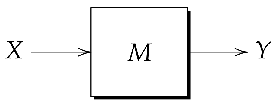
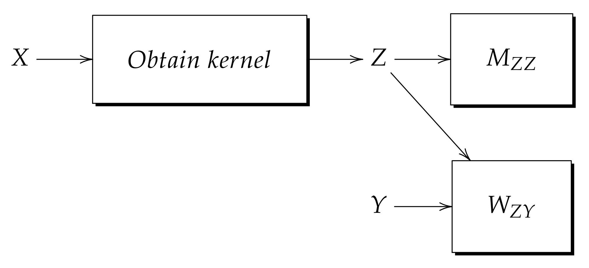
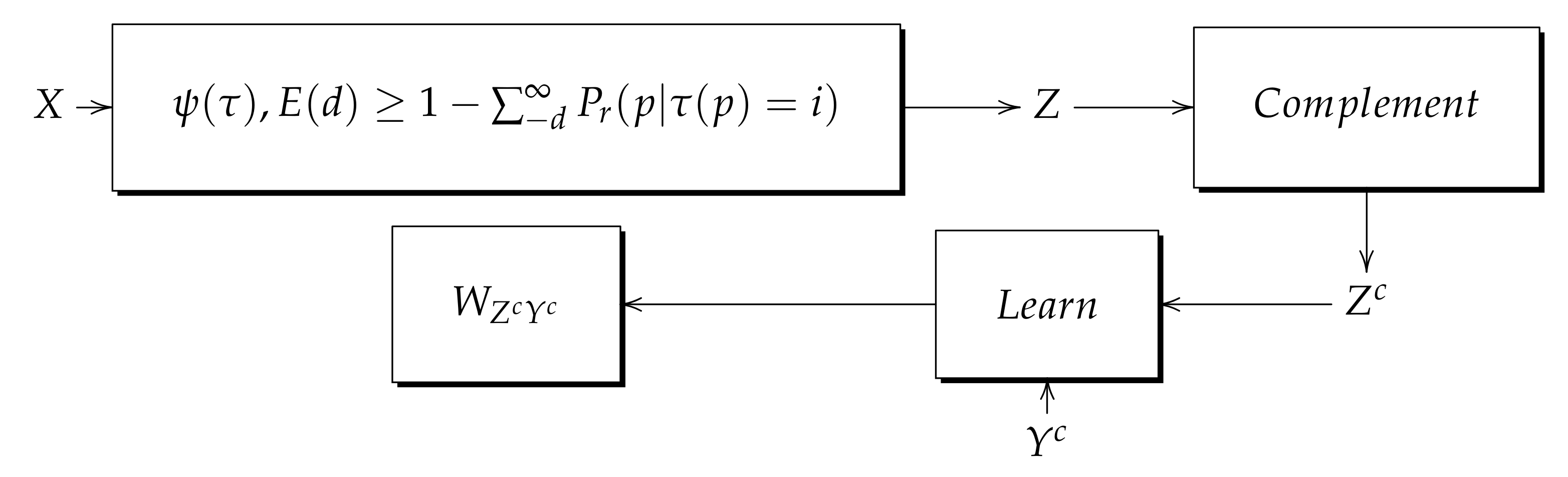
- Learning phase: The diagram in Figure 3 shows the learning phase of the kernel model. As seen in the figure, the input pattern X enters a process that obtains , then, Z is autoassociatively learned with memory M; furthermore, Z is heteroassociatively learned with output pattern Y but this time with memory W.
- 2.
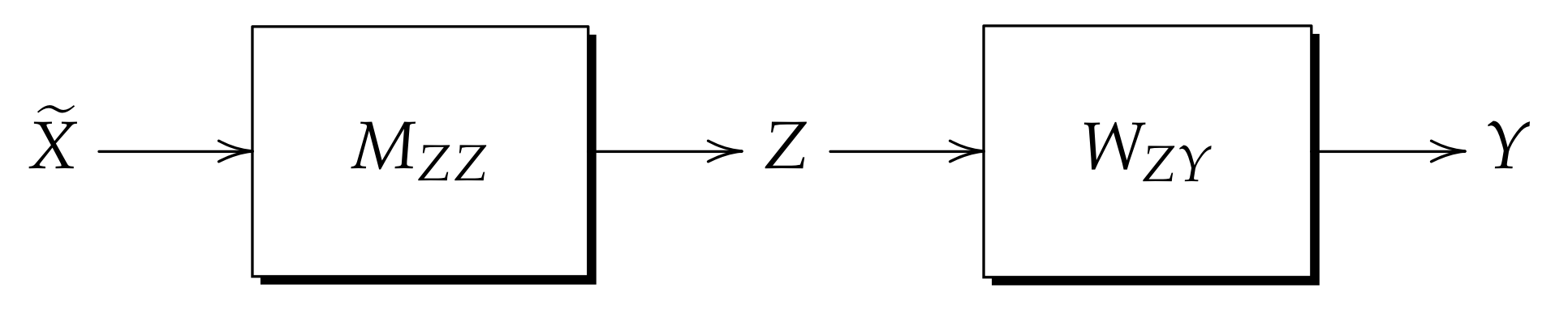
- Recall phase: Figure 4 shows the process followed when applying the recall phase in the kernel model. Given as the mixed noise-distorted version of the learned pattern X, is presented to memory and Z is recalled, immediately afterwards, Z is presented to Memory and as a result the output pattern Y is recalled.
1.4. Fast Distance Transform (FDT)
- 1.
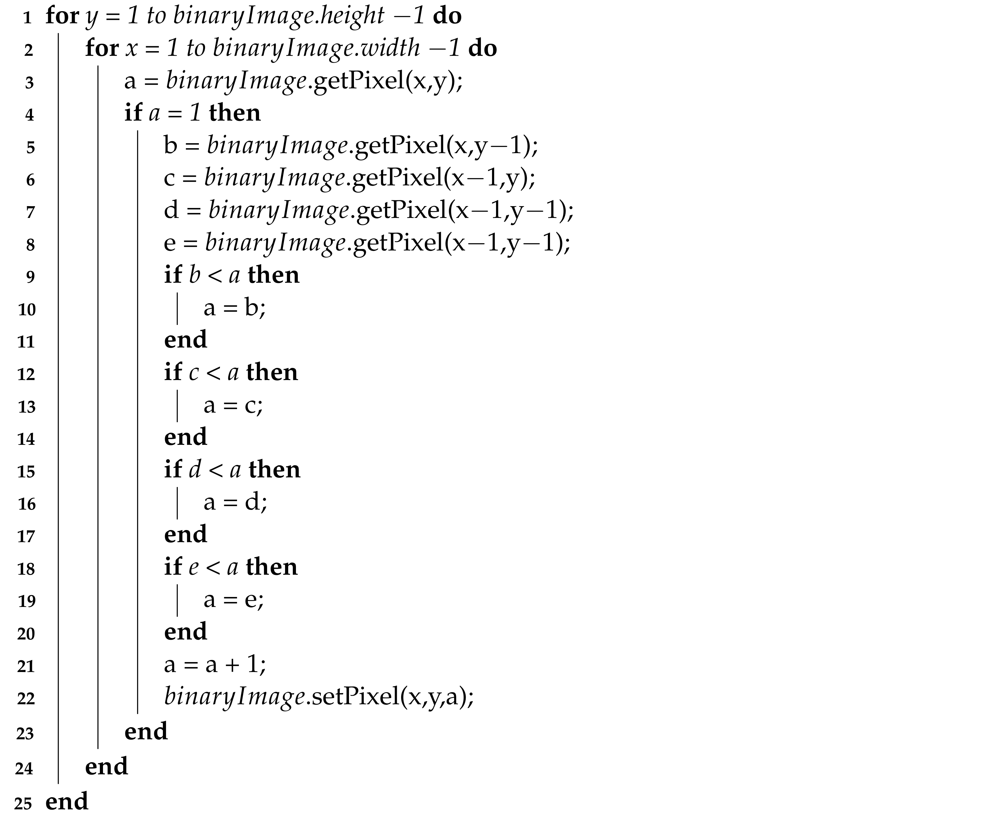
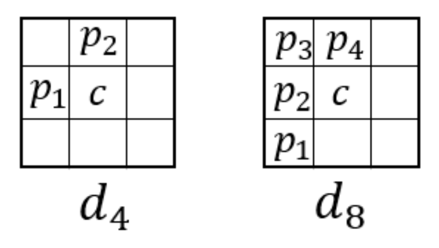
- Read each pixel in the binary image from top to bottom and from left to right, then, each pixel , where R is the region of interest, is assigned as presented in Equation (19). Algorithm 1 illustrates the pseudocode of this same Equation (19).E is one of the following sets shown in Figure 5. Only the points assigned in E are used in the first part of the transformation.
- 2.
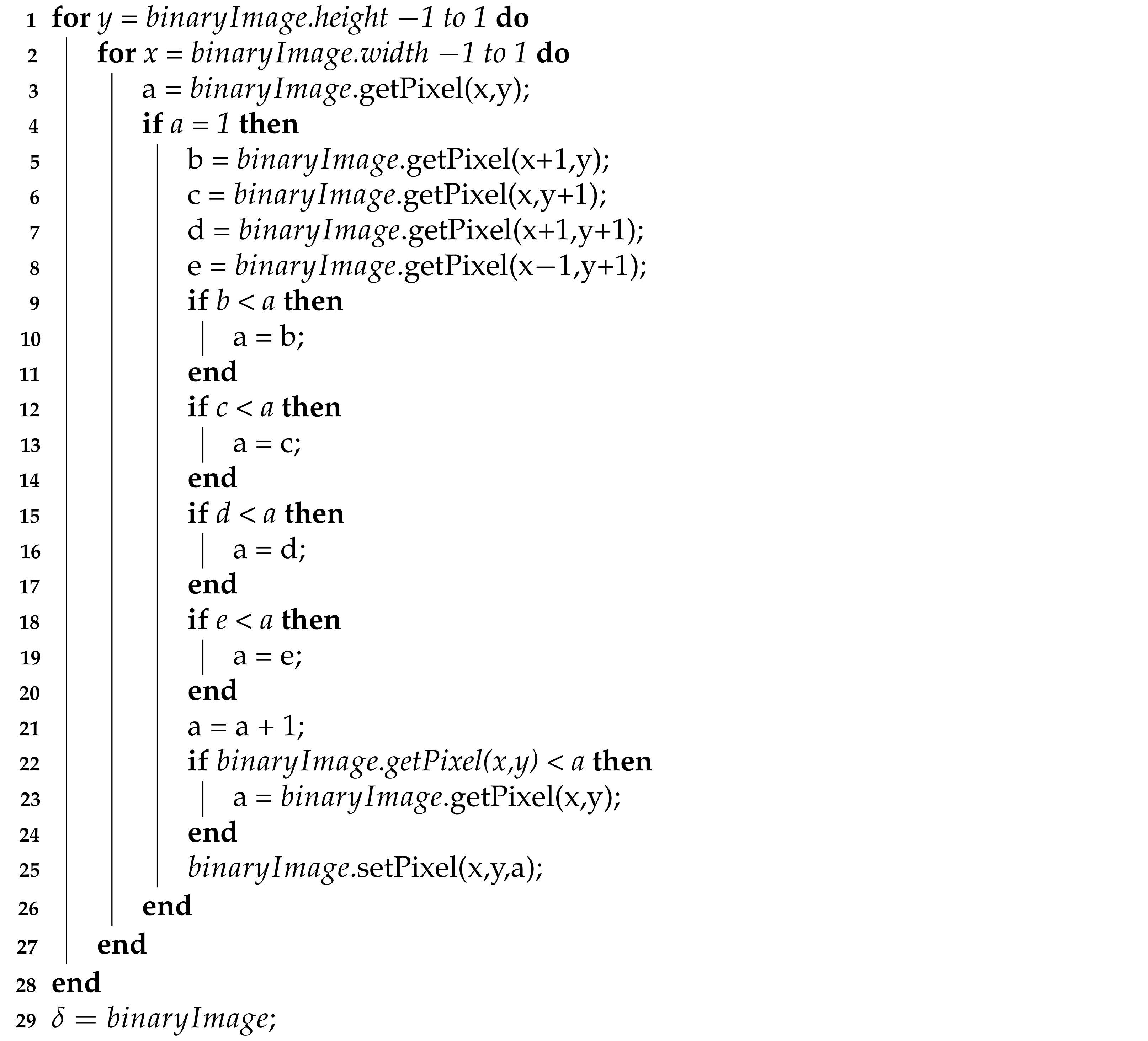
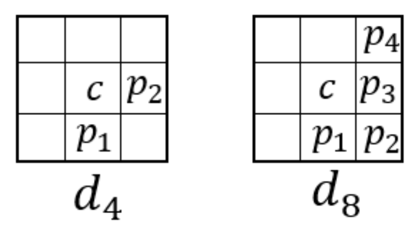
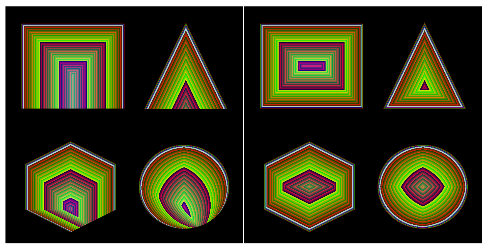
- Read the binary image from bottom to top and from right to left, then, each pixel , where R is the region of interest, is assigned as shown in Equation (20). Algorithm 2 illustrates the pseudocode of this same Equation (20).D is one of the sets shown in Figure 6. Note that, only the points assigned in D are used in the first part of the transformation.Figure 7 illustrates the result of the two steps of the FDT.
| Algorithm 1 FDT algorithm first step with the metrics. |
 |
| Algorithm 2 FDT algorithm second step with the metrics. |
 |
2. Materials and Methods
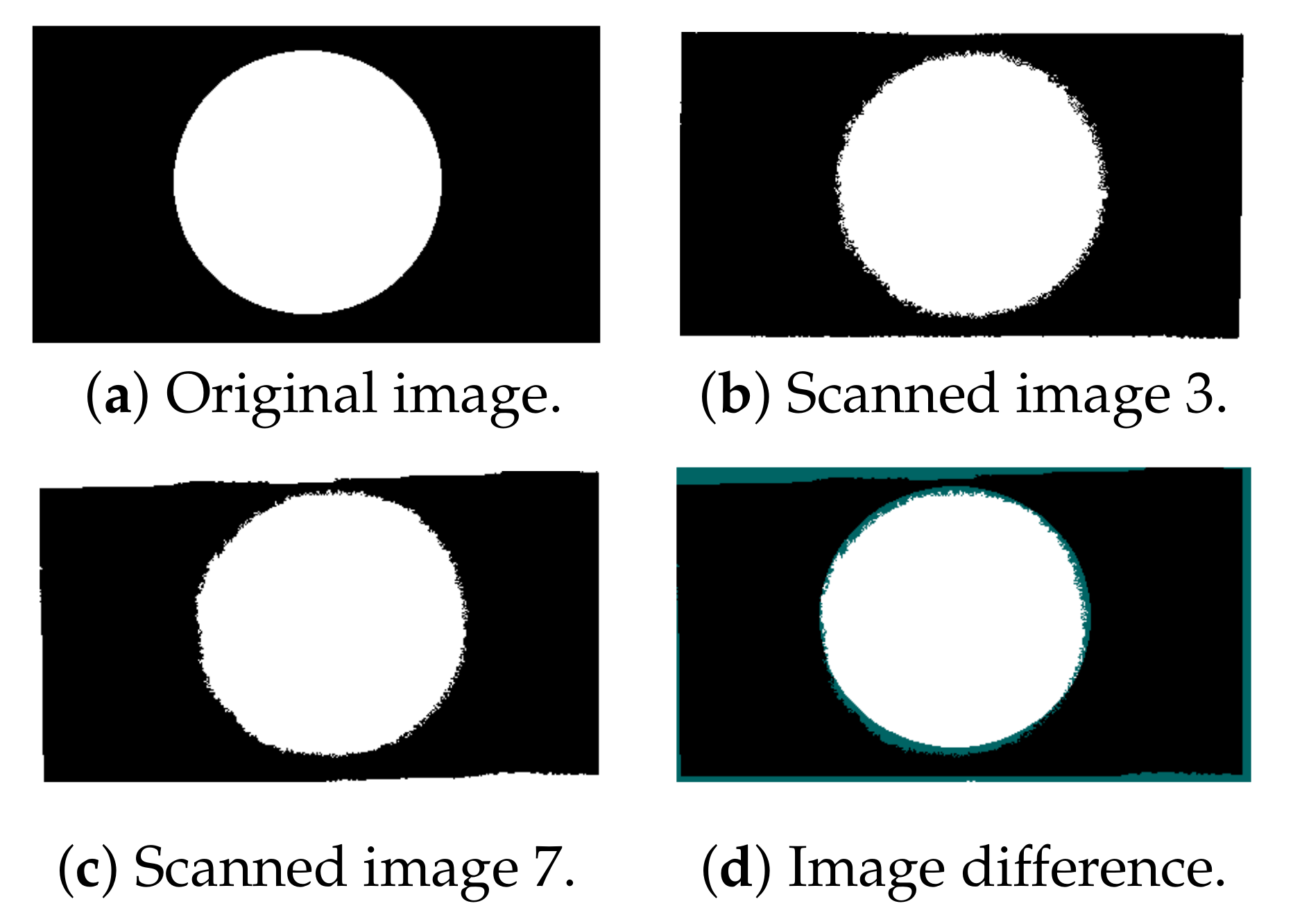
2.1. Noise
- 1.
- Print the binary image on paper.
- 2.
- Scan the image obtained from step 1, generating a new digital image.
- 3.
- Compare the new digital image with the original one and store the percentage difference.
- 4.
- Print the new digital image obtained in step 2.
- 5.
- Repeat steps 2 to 4, 15 times with 80 different images (40 binary images and 40 gray -scale images ).
- with 64 dpi resolution.
- with 180 dpi resolution
- with 96 dpi resolution.
| Algorithm 3 Noise probability distribution algorithm for binary images. |
 |
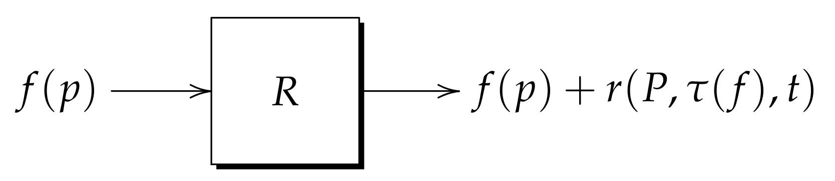
- is a time-dependent random function of t and independent from f.
- is a random function depending on a measure τ taken from the obtained data.
- is a p-dependent random function of -domain of the noisy information.
| Algorithm 4 Mixed noise simulation algorithm for binary images. |
 |
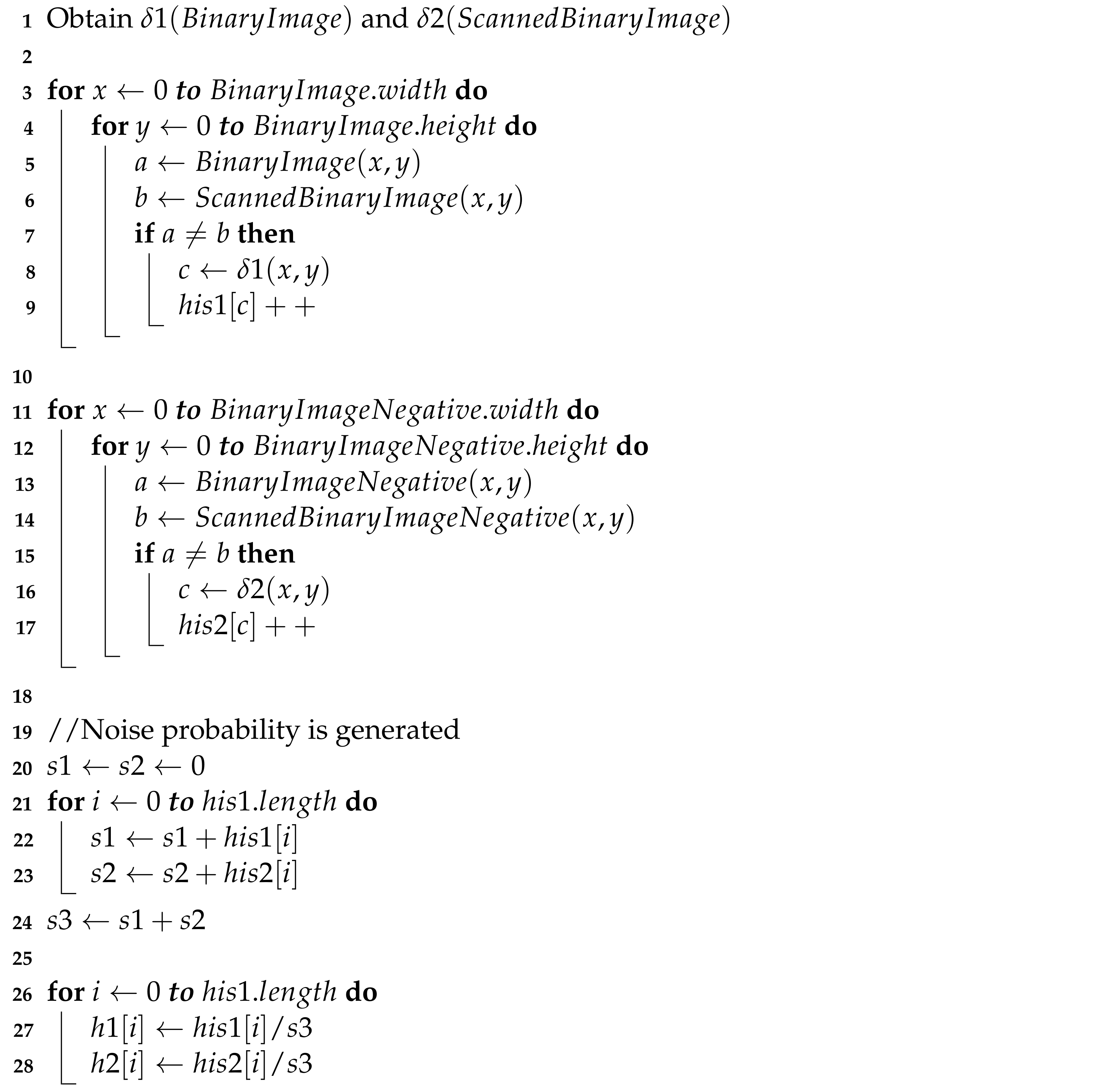
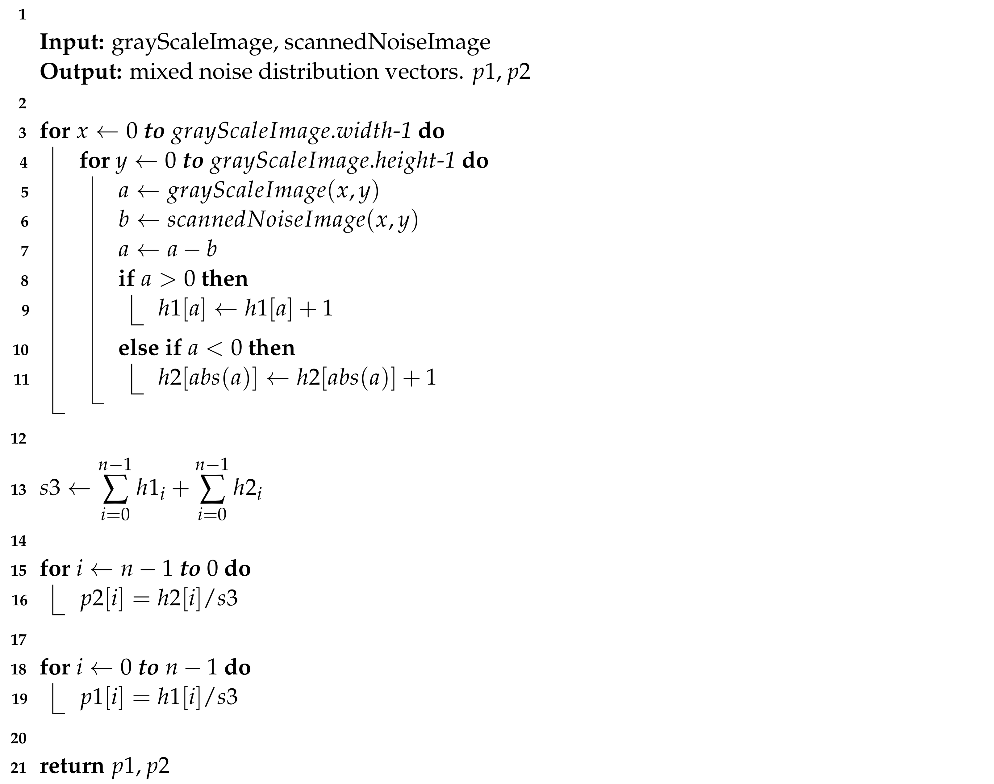
| Algorithm 5 Algorithm that obtains the probability distribution of the acquisition noise. |
 |
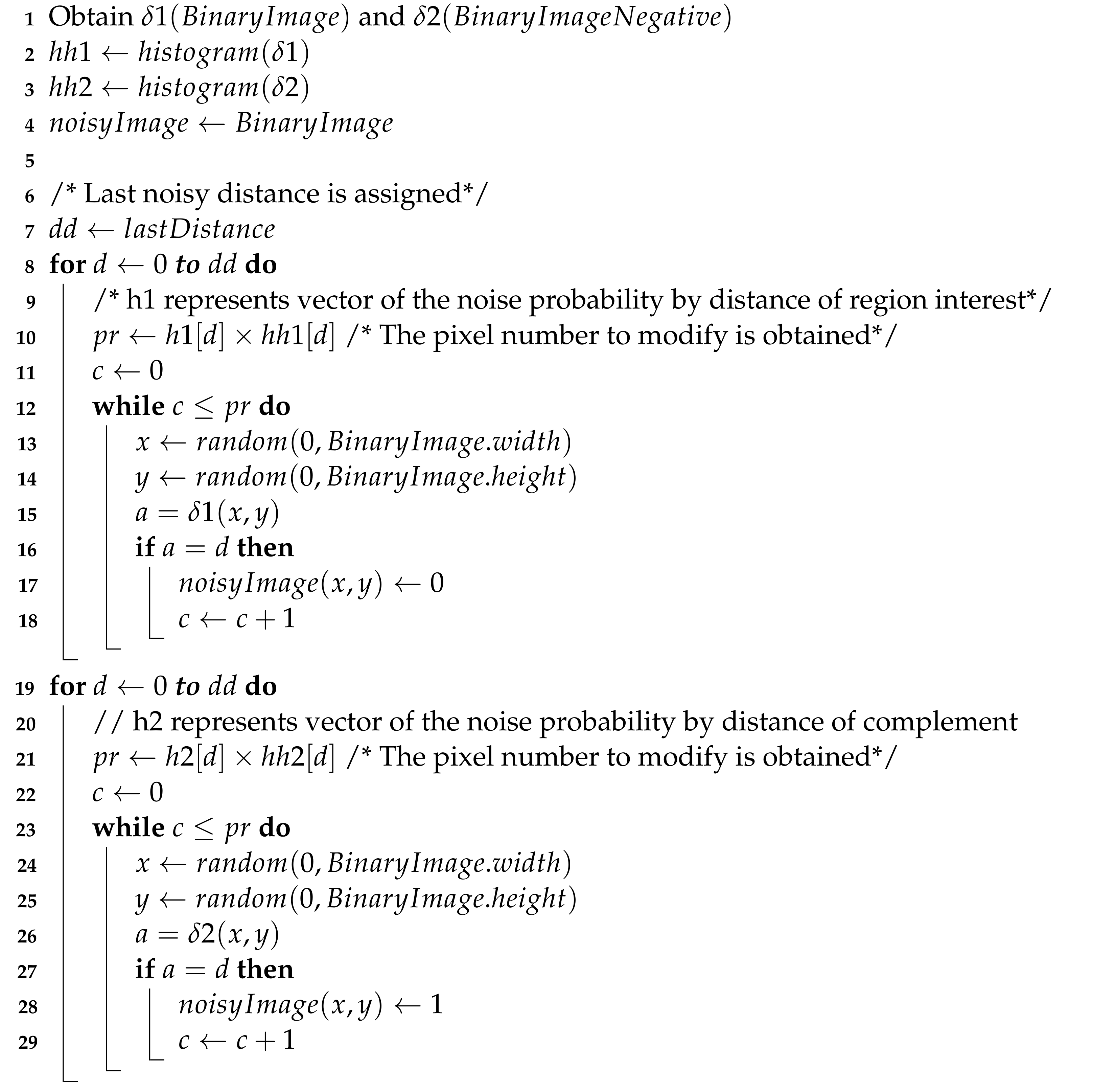
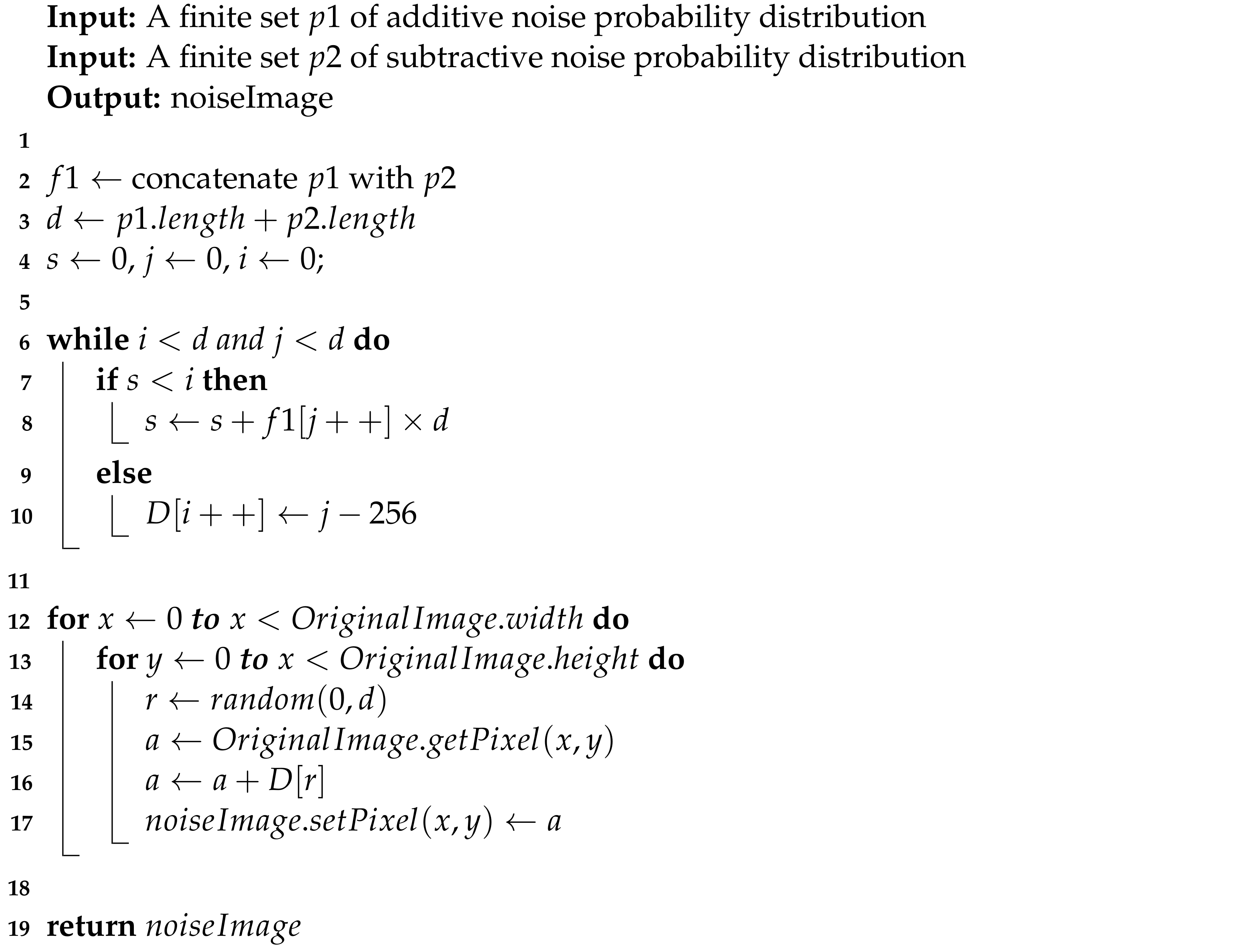
| Algorithm 6 Image with simulated mixed noise. |
 |
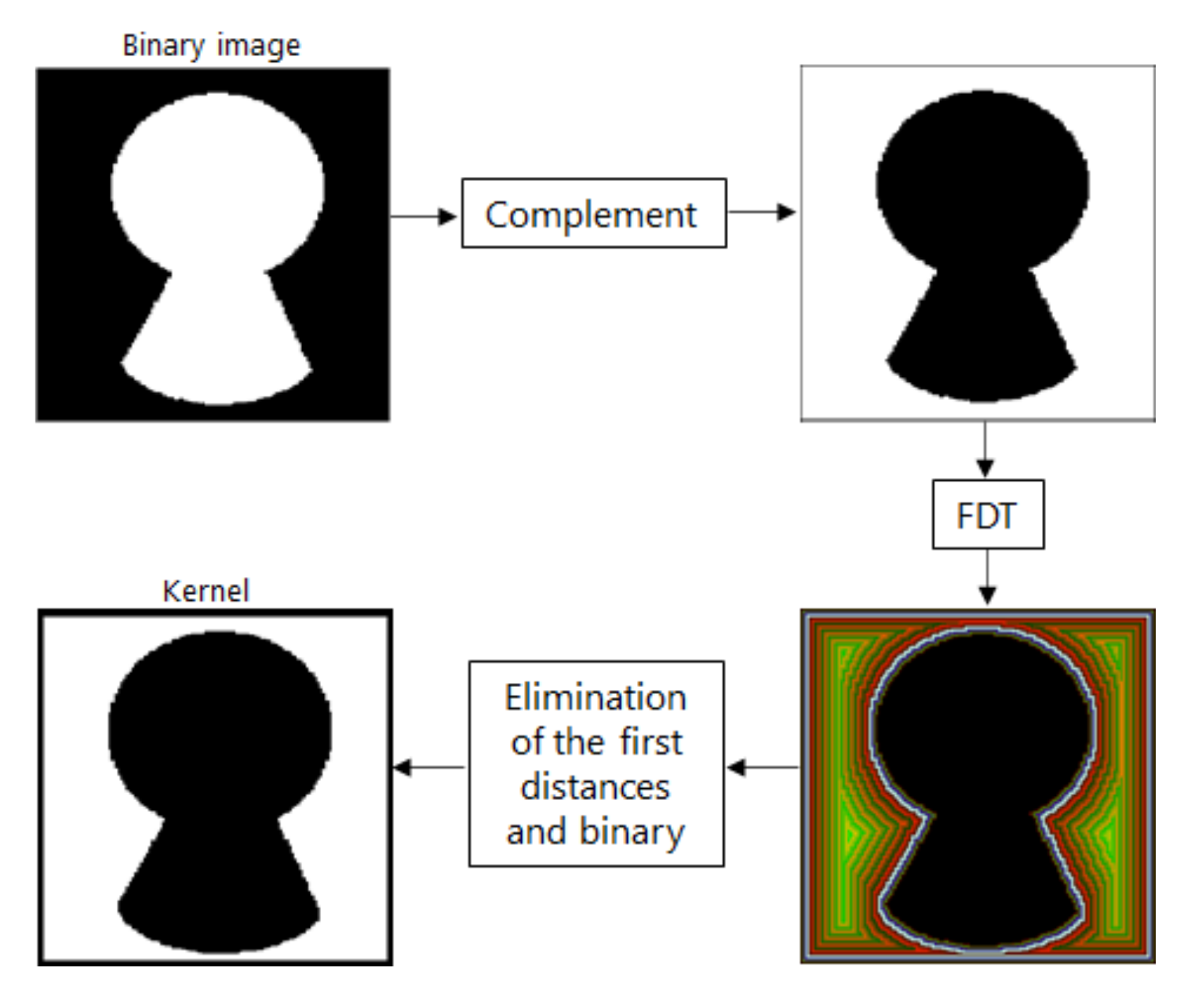
2.2. Optimal Kernel Based on FDT
- 1.
- Erode up to distance of .
- 2.
- Binarize the eroded .
- 3.
- Obtain the complement of the eroded image from step 2.
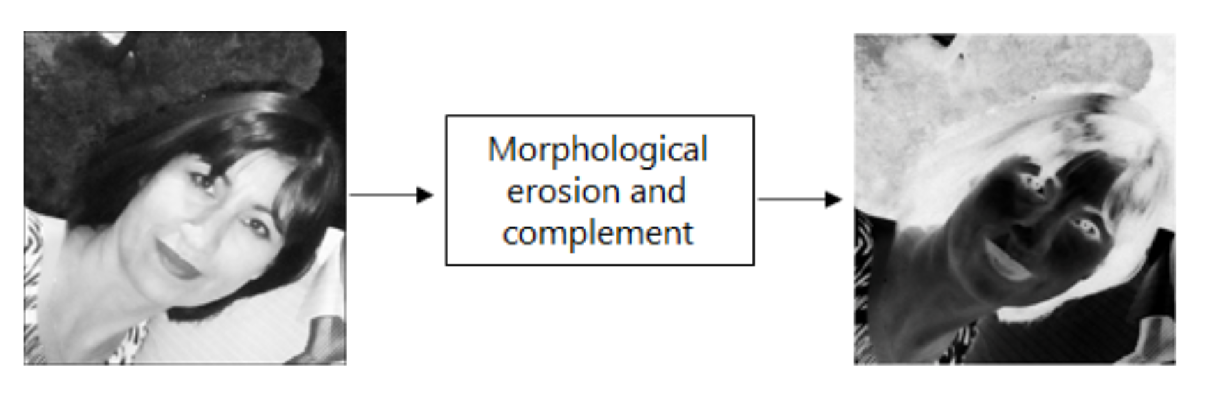
- 1.
- Erode the image.
- 2.
- Obtain the complement of the eroded image.
2.2.1. Learning Phase
2.2.2. Recall Phase
2.2.3. New Generic Model of Min Heteroassociative Memories Robust to Mixed Noise
- 1.
- Obtain by and Theorem 3.
- 2.
- Obtain the Z complement ().
- 3.
- Obtain the Y complement ().
- 4.
- Perform the learning process with .
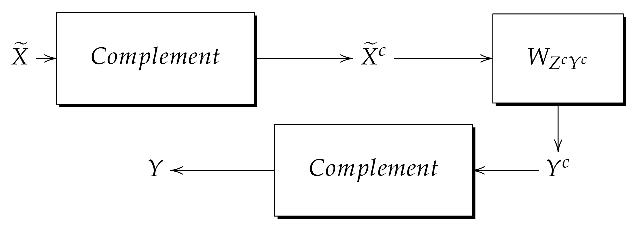
- 1.
- Obtain the complement.
- 2.
- Perform the recall process with memory .
- 3.
- Obtain the complement.
3. Results
3.1. Acquisition Noise Distribution
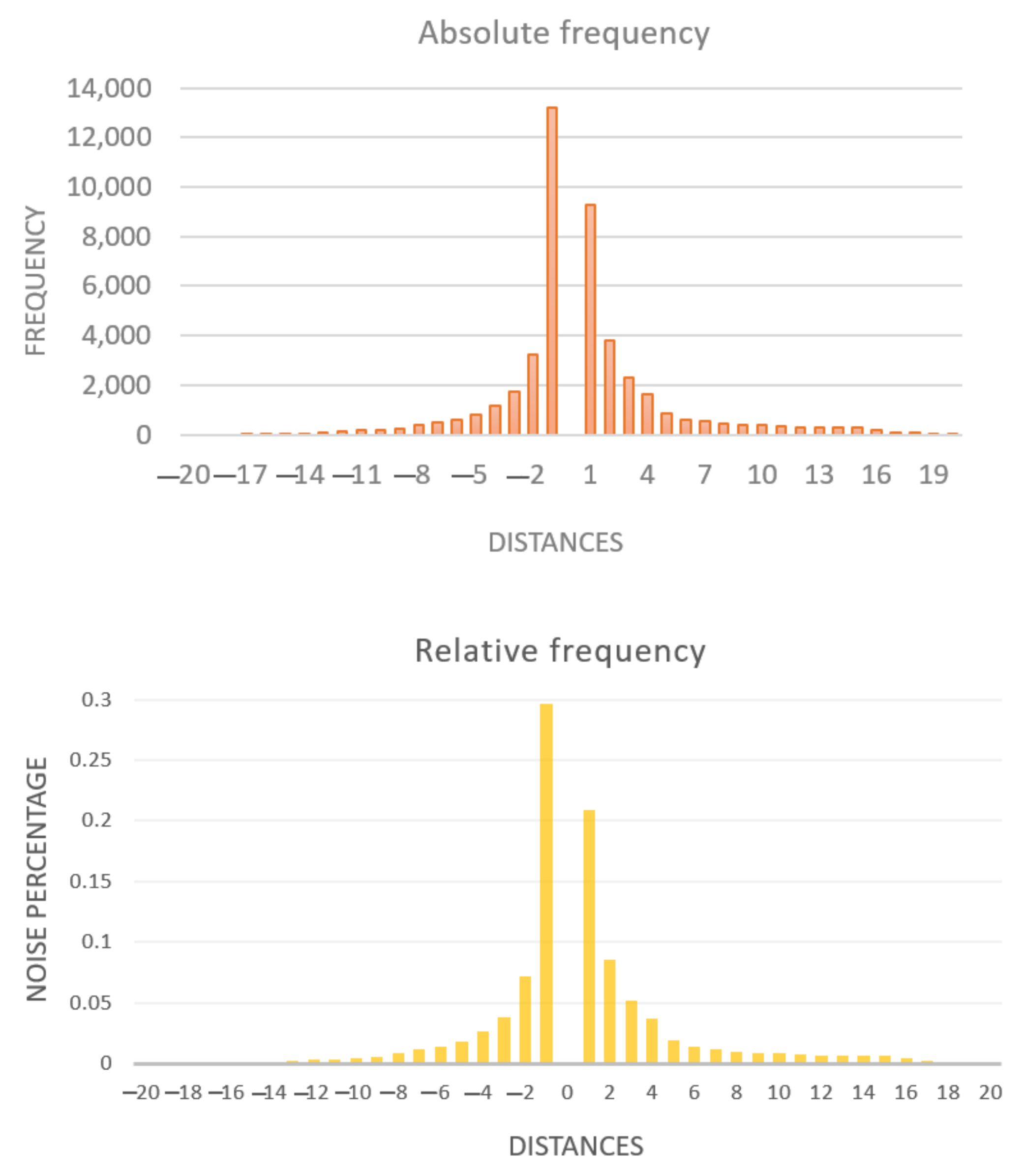
3.1.1. Acquisition Noise Distribution in Binary Images
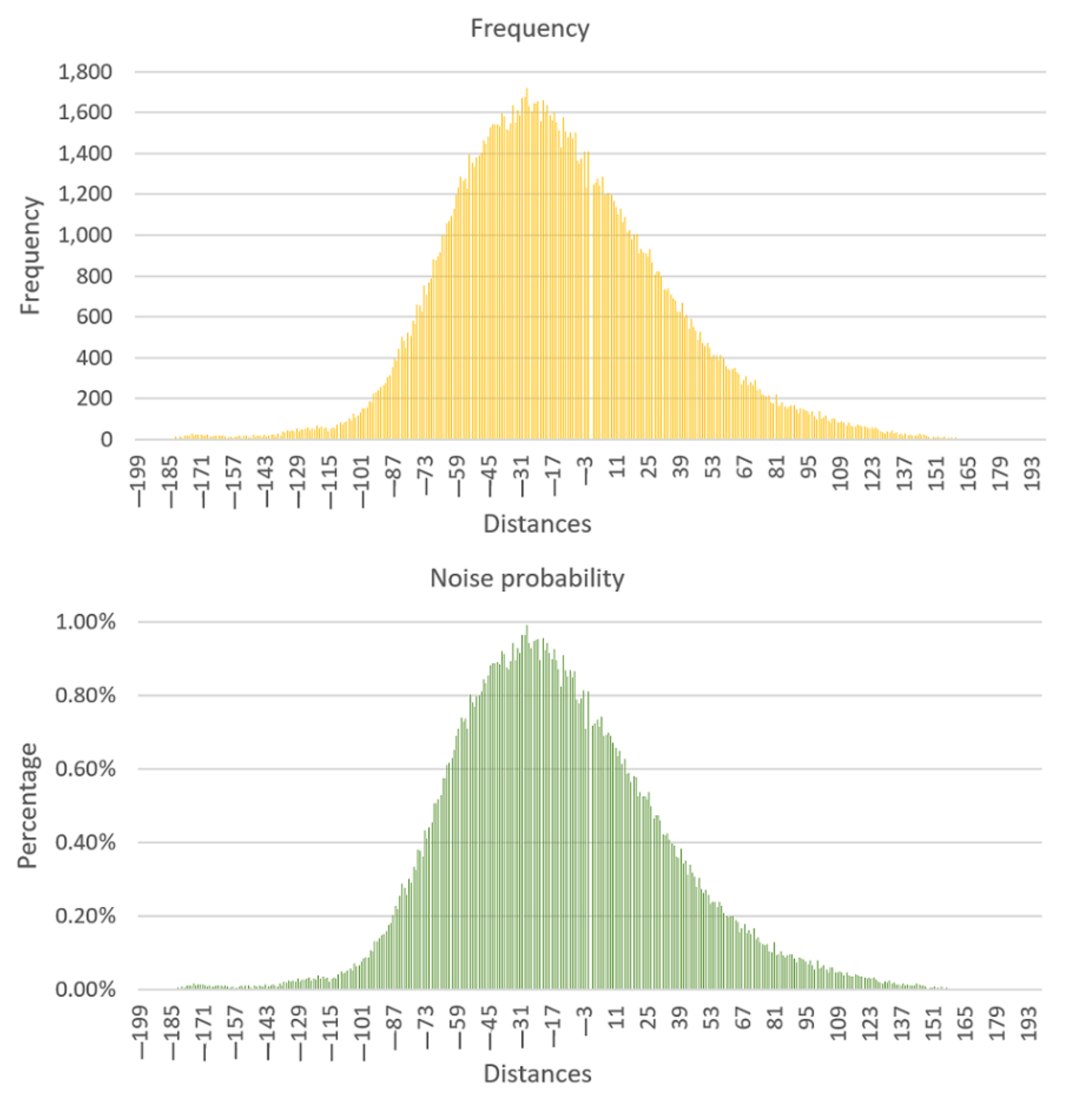
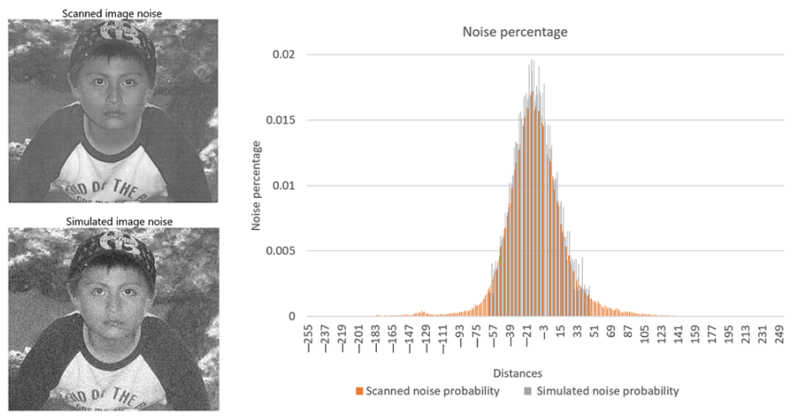
3.1.2. Acquisition Noise Distribution in Grayscale Images
3.2. New Model of Min Heteroassociative Memory
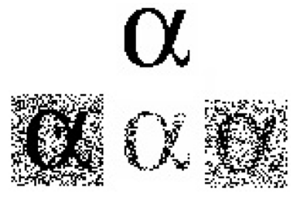
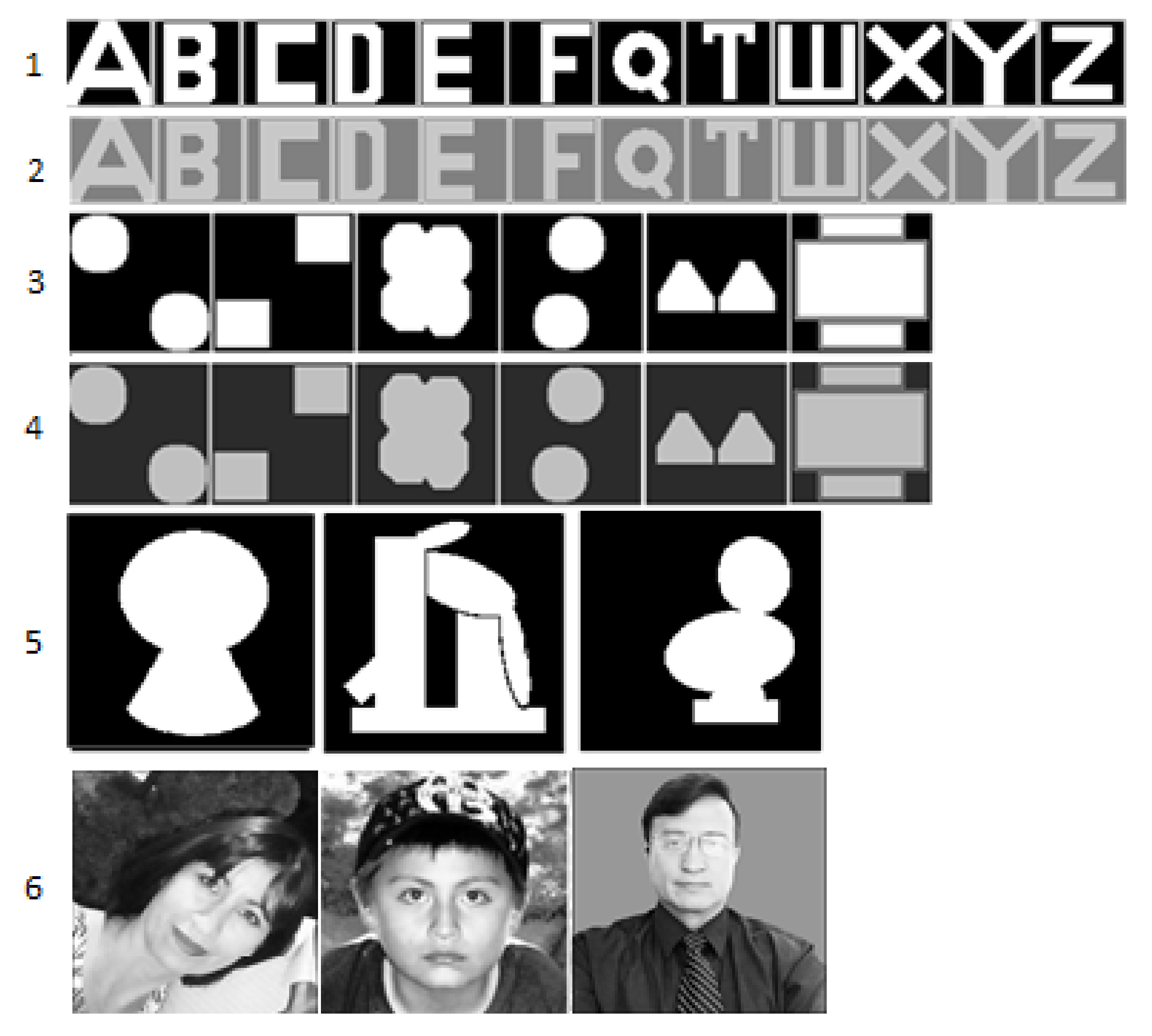
- 6 fundamental sets, 3 with binary images and 3 with grayscale images. Figure 16 shows the fundamental sets appearance.
- The images of fundamental set 1 and 2 are of size , those of set 3 and 4 are , while those of set 5 and 6 are .
- Table 4 shows how far away the kernel will be created.
- 1000 recall process per fundamental set.
4. Discussion
5. Conclusions
Author Contributions
Funding
Institutional Review Board Statement
Informed Consent Statement
Data Availability Statement
Acknowledgments
Conflicts of Interest
Appendix A. Acquisition Noise Distribution Table in Grayscale Images

| Distance | Frequency | Probability | Distance | Frequency | Probability |
|---|---|---|---|---|---|
| −189 | 3 | 0.00000173 | −94 | 231 | 0.001332764 |
| −188 | 3 | 0.00000173 | −93 | 242 | 0.001396229 |
| −187 | 2 | 0.00000115 | −92 | 257 | 0.001482772 |
| −186 | 3 | 0.00000173 | −91 | 263 | 0.001517389 |
| −185 | 4 | 0.00000231 | −90 | 276 | 0.001592393 |
| −184 | 5 | 0.00000288 | −89 | 305 | 0.00175971 |
| −183 | 6 | 0.00000346 | −88 | 314 | 0.001811636 |
| −182 | 12 | 0.00000692 | −87 | 353 | 0.002036648 |
| −181 | 6 | 0.00000346 | −86 | 397 | 0.002290508 |
| −180 | 16 | 0.00000923 | −85 | 383 | 0.002209734 |
| −179 | 9 | 0.00000519 | −84 | 442 | 0.002550137 |
| −178 | 21 | 0.00012116 | −83 | 500 | 0.002884771 |
| −177 | 18 | 0.000103852 | −82 | 480 | 0.00276938 |
| −176 | 20 | 0.000115391 | −81 | 449 | 0.002590524 |
| −175 | 30 | 0.000173086 | −80 | 524 | 0.00302324 |
| −174 | 20 | 0.000115391 | −79 | 505 | 0.002913618 |
| −173 | 23 | 0.000132699 | −78 | 581 | 0.003352104 |
| −172 | 23 | 0.000132699 | −77 | 568 | 0.0032771 |
| −171 | 25 | 0.000144239 | −76 | 661 | 0.003813667 |
| −170 | 18 | 0.000103852 | −75 | 654 | 0.00377328 |
| −169 | 17 | 0.00000981 | −74 | 627 | 0.003617502 |
| −168 | 22 | 0.00012693 | −73 | 752 | 0.004338695 |
| −167 | 15 | 0.00000865 | −72 | 711 | 0.004102144 |
| −166 | 14 | 0.00000808 | −71 | 767 | 0.004425238 |
| −165 | 19 | 0.000109621 | −70 | 788 | 0.004546399 |
| −164 | 18 | 0.000103852 | −69 | 880 | 0.005077196 |
| −163 | 19 | 0.000109621 | −68 | 878 | 0.005065657 |
| −162 | 17 | 0.00000981 | −67 | 898 | 0.005181048 |
| −161 | 21 | 0.00012116 | −66 | 918 | 0.005296439 |
| −160 | 13 | 0.00000750 | −65 | 998 | 0.005758002 |
| −159 | 10 | 0.00000577 | −64 | 999 | 0.005763772 |
| −158 | 13 | 0.00000750 | −63 | 1060 | 0.006115714 |
| −157 | 8 | 0.00000462 | −62 | 1071 | 0.006179179 |
| −156 | 12 | 0.00000692 | −61 | 1091 | 0.00629457 |
| −155 | 15 | 0.00000865 | −60 | 1130 | 0.006519582 |
| −154 | 18 | 0.000103852 | −59 | 1198 | 0.006911911 |
| −153 | 11 | 0.00000635 | −58 | 1230 | 0.007096536 |
| −152 | 19 | 0.000109621 | −57 | 1284 | 0.007408091 |
| −151 | 18 | 0.000103852 | −56 | 1265 | 0.00729847 |
| −150 | 10 | 0.00000577 | −55 | 1278 | 0.007373474 |
| −149 | 7 | 0.00000404 | −54 | 1228 | 0.007084997 |
| −148 | 22 | 0.00012693 | −53 | 1393 | 0.008036971 |
| −147 | 16 | 0.00000923 | −52 | 1353 | 0.00780619 |
| −146 | 20 | 0.000115391 | −51 | 1334 | 0.007696568 |
| −145 | 17 | 0.00000981 | −50 | 1381 | 0.007967737 |
| −144 | 16 | 0.00000923 | −49 | 1389 | 0.008013893 |
| −143 | 24 | 0.000138469 | −48 | 1404 | 0.008100436 |
| −142 | 16 | 0.00000923 | −47 | 1463 | 0.008440839 |
| −141 | 19 | 0.000109621 | −46 | 1446 | 0.008342757 |
| −140 | 23 | 0.000132699 | −45 | 1483 | 0.00855623 |
| −139 | 22 | 0.00012693 | −44 | 1527 | 0.00881009 |
| −138 | 13 | 0.00000750 | −43 | 1540 | 0.008885094 |
| −137 | 28 | 0.000161547 | −42 | 1540 | 0.008885094 |
| −136 | 20 | 0.000115391 | −41 | 1544 | 0.008908172 |
| −135 | 39 | 0.000225012 | −40 | 1534 | 0.008850477 |
| −134 | 36 | 0.000207703 | −39 | 1596 | 0.009208188 |
| −133 | 42 | 0.000242321 | −38 | 1583 | 0.009133184 |
| −132 | 39 | 0.000225012 | −37 | 1518 | 0.008758164 |
| −131 | 43 | 0.00024809 | −36 | 1511 | 0.008717777 |
| −130 | 39 | 0.000225012 | −35 | 1548 | 0.00893125 |
| −129 | 54 | 0.000311555 | −34 | 1634 | 0.009427431 |
| −128 | 40 | 0.000230782 | −33 | 1554 | 0.008965867 |
| −127 | 49 | 0.000282708 | −32 | 1612 | 0.009300501 |
| −126 | 48 | 0.000276938 | −31 | 1585 | 0.009144723 |
| −125 | 54 | 0.000311555 | −30 | 1671 | 0.009640904 |
| −124 | 59 | 0.000340403 | −29 | 1673 | 0.009652443 |
| −123 | 45 | 0.000259629 | −28 | 1719 | 0.009917842 |
| −122 | 54 | 0.000311555 | −27 | 1632 | 0.009415892 |
| −121 | 47 | 0.000271168 | −26 | 1608 | 0.009277423 |
| −120 | 69 | 0.000398098 | −25 | 1644 | 0.009485126 |
| −119 | 51 | 0.000294247 | −24 | 1647 | 0.009502435 |
| −118 | 64 | 0.000369251 | −23 | 1655 | 0.009548591 |
| −117 | 53 | 0.000305786 | −22 | 1555 | 0.008971637 |
| −116 | 59 | 0.000340403 | −21 | 1659 | 0.009571669 |
| −115 | 39 | 0.000225012 | −20 | 1600 | 0.009231266 |
| −114 | 51 | 0.000294247 | −19 | 1635 | 0.0094332 |
| −113 | 60 | 0.000346172 | −18 | 1586 | 0.009150493 |
| −112 | 54 | 0.000311555 | −17 | 1560 | 0.009000485 |
| −111 | 73 | 0.000421177 | −16 | 1603 | 0.009248575 |
| −110 | 85 | 0.000490411 | −15 | 1552 | 0.008954328 |
| −109 | 75 | 0.000432716 | −14 | 1511 | 0.008717777 |
| −108 | 82 | 0.000473102 | −13 | 1429 | 0.008244675 |
| −107 | 90 | 0.000519259 | −12 | 1578 | 0.009104336 |
| −106 | 101 | 0.000582724 | −11 | 1505 | 0.00868316 |
| −105 | 91 | 0.000525028 | −10 | 1479 | 0.008533152 |
| −104 | 125 | 0.000721193 | −9 | 1504 | 0.00867739 |
| −103 | 108 | 0.00062311 | −8 | 1472 | 0.008492765 |
| −102 | 117 | 0.000675036 | −7 | 1502 | 0.008665851 |
| −101 | 133 | 0.000767349 | −6 | 1366 | 0.007881194 |
| −100 | 150 | 0.000865431 | −5 | 1349 | 0.007783111 |
| −99 | 151 | 0.000871201 | −4 | 1374 | 0.00792735 |
| −98 | 155 | 0.000894279 | −3 | 1409 | 0.008129284 |
| −97 | 184 | 0.001061596 | −2 | 1232 | 0.007108075 |
| −96 | 183 | 0.001055826 | −1 | 1408 | 0.008123514 |
| −95 | 228 | 0.001315455 | 0 | 0 | 0 |
| Distance | Frequency | Probability | Distance | Frequency | Probability |
|---|---|---|---|---|---|
| 1 | 1245 | 0.007183079 | 95 | 135 | 0.000778888 |
| 2 | 1256 | 0.007246544 | 96 | 120 | 0.000692345 |
| 3 | 1274 | 0.007350396 | 97 | 137 | 0.000790427 |
| 4 | 1239 | 0.007148462 | 98 | 113 | 0.000651958 |
| 5 | 1285 | 0.007413861 | 99 | 96 | 0.000553876 |
| 6 | 1197 | 0.006906141 | 100 | 137 | 0.000790427 |
| 7 | 1200 | 0.00692345 | 101 | 102 | 0.000588493 |
| 8 | 1209 | 0.006975376 | 102 | 107 | 0.000617341 |
| 9 | 1198 | 0.006911911 | 103 | 116 | 0.000669267 |
| 10 | 1166 | 0.006727285 | 104 | 94 | 0.000542337 |
| 11 | 1139 | 0.006571508 | 105 | 82 | 0.000473102 |
| 12 | 1103 | 0.006363804 | 106 | 104 | 0.000600032 |
| 13 | 1126 | 0.006496504 | 107 | 104 | 0.000600032 |
| 14 | 1064 | 0.006138792 | 108 | 83 | 0.000478872 |
| 15 | 1086 | 0.006265722 | 109 | 81 | 0.000467333 |
| 16 | 1016 | 0.005861854 | 110 | 87 | 0.00050195 |
| 17 | 1023 | 0.005902241 | 111 | 81 | 0.000467333 |
| 18 | 979 | 0.005648381 | 112 | 67 | 0.000386559 |
| 19 | 1005 | 0.005798389 | 113 | 82 | 0.000473102 |
| 20 | 1003 | 0.00578685 | 114 | 69 | 0.000398098 |
| 21 | 911 | 0.005256052 | 115 | 64 | 0.000369251 |
| 22 | 933 | 0.005382982 | 116 | 62 | 0.000357712 |
| 23 | 914 | 0.005273361 | 117 | 73 | 0.000421177 |
| 24 | 912 | 0.005261822 | 118 | 69 | 0.000398098 |
| 25 | 897 | 0.005175279 | 119 | 61 | 0.000351942 |
| 26 | 933 | 0.005382982 | 120 | 64 | 0.000369251 |
| 27 | 867 | 0.005002192 | 121 | 56 | 0.000323094 |
| 28 | 807 | 0.00465602 | 122 | 53 | 0.000305786 |
| 29 | 821 | 0.004736794 | 123 | 60 | 0.000346172 |
| 30 | 822 | 0.004742563 | 124 | 52 | 0.000300016 |
| 31 | 797 | 0.004598325 | 125 | 59 | 0.000340403 |
| 32 | 734 | 0.004234843 | 126 | 48 | 0.000276938 |
| 33 | 727 | 0.004194457 | 127 | 38 | 0.000219243 |
| 34 | 737 | 0.004252152 | 128 | 35 | 0.000201934 |
| 35 | 710 | 0.004096374 | 129 | 29 | 0.000167317 |
| 36 | 689 | 0.003975214 | 130 | 39 | 0.000225012 |
| 37 | 679 | 0.003917519 | 131 | 36 | 0.000207703 |
| 38 | 626 | 0.003611733 | 132 | 43 | 0.00024809 |
| 39 | 625 | 0.003605963 | 133 | 29 | 0.000167317 |
| 40 | 667 | 0.003848284 | 134 | 35 | 0.000201934 |
| 41 | 596 | 0.003438647 | 135 | 26 | 0.000150008 |
| 42 | 608 | 0.003507881 | 136 | 27 | 0.000155778 |
| 43 | 542 | 0.003127091 | 137 | 20 | 0.000115391 |
| 44 | 591 | 0.003409799 | 138 | 29 | 0.000167317 |
| 45 | 552 | 0.003184787 | 139 | 20 | 0.000115391 |
| 46 | 532 | 0.003069396 | 140 | 23 | 0.000132699 |
| 47 | 486 | 0.002803997 | 141 | 19 | 0.000109621 |
| 48 | 526 | 0.003034779 | 142 | 18 | 0.000103852 |
| 49 | 474 | 0.002734763 | 143 | 18 | 0.000103852 |
| 50 | 459 | 0.00264822 | 144 | 30 | 0.000173086 |
| 51 | 470 | 0.002711684 | 145 | 26 | 0.000150008 |
| 52 | 449 | 0.002590524 | 146 | 22 | 0.00012693 |
| 53 | 403 | 0.002325125 | 147 | 18 | 0.000103852 |
| 54 | 413 | 0.002382821 | 148 | 16 | 0.00000923 |
| 55 | 415 | 0.00239436 | 149 | 6 | 0.00000346 |
| 56 | 388 | 0.002238582 | 150 | 12 | 0.00000692 |
| 57 | 414 | 0.00238859 | 151 | 10 | 0.00000577 |
| 58 | 397 | 0.002290508 | 152 | 13 | 0.00000750 |
| 59 | 360 | 0.002077035 | 153 | 10 | 0.00000577 |
| 60 | 346 | 0.001996261 | 154 | 8 | 0.00000462 |
| 61 | 341 | 0.001967414 | 155 | 13 | 0.00000750 |
| 62 | 346 | 0.001996261 | 156 | 6 | 0.00000346 |
| 63 | 347 | 0.002002031 | 157 | 9 | 0.00000519 |
| 64 | 327 | 0.00188664 | 158 | 8 | 0.00000462 |
| 65 | 320 | 0.001846253 | 159 | 4 | 0.00000231 |
| 66 | 271 | 0.001563546 | 160 | 7 | 0.00000404 |
| 67 | 292 | 0.001684706 | 161 | 6 | 0.00000346 |
| 68 | 310 | 0.001788558 | 162 | 3 | 0.00000173 |
| 69 | 266 | 0.001534698 | 163 | 4 | 0.00000231 |
| 70 | 279 | 0.001609702 | 164 | 5 | 0.00000288 |
| 71 | 263 | 0.001517389 | 165 | 2 | 0.00000115 |
| 72 | 290 | 0.001673167 | 166 | 2 | 0.00000115 |
| 73 | 240 | 0.00138469 | 167 | 5 | 0.00000288 |
| 74 | 246 | 0.001419307 | 168 | 5 | 0.00000288 |
| 75 | 223 | 0.001286608 | 169 | 1 | 0.00000577 |
| 76 | 215 | 0.001240451 | 170 | 2 | 0.00000115 |
| 77 | 211 | 0.001217373 | 171 | 1 | 0.000000577 |
| 78 | 215 | 0.001240451 | 172 | 3 | 0.00000173 |
| 79 | 181 | 0.001044287 | 173 | 2 | 0.00000115 |
| 80 | 179 | 0.001032748 | 174 | 1 | 0.000000577 |
| 81 | 222 | 0.001280838 | 175 | 2 | 0.00000115 |
| 82 | 161 | 0.000928896 | 176 | 0 | 0 |
| 83 | 167 | 0.000963513 | 177 | 0 | 0 |
| 84 | 183 | 0.001055826 | 178 | 2 | 0.00000115 |
| 85 | 164 | 0.000946205 | 179 | 2 | 0.00000115 |
| 86 | 154 | 0.000888509 | 180 | 0 | 0 |
| 87 | 161 | 0.000928896 | 181 | 1 | 0.000000577 |
| 88 | 168 | 0.000969283 | 182 | 0 | 0 |
| 89 | 166 | 0.000957744 | 183 | 1 | 0.000000577 |
| 90 | 147 | 0.000848123 | 184 | 0 | 0 |
| 91 | 127 | 0.000732732 | 185 | 0 | 0 |
| 92 | 153 | 0.00088274 | 186 | 0 | 0 |
| 93 | 149 | 0.000859662 | 187 | 1 | 0.000000577 |
| 94 | 144 | 0.000830814 |
References
- Steinbuch, K. Die Lernmatrix. Kybernetik 1961, 1, 36–45. [Google Scholar] [CrossRef]
- Willshaw, D.; Buneman, O.; Longuet-Higgins, H. Non-holographic associative memory. Nature 1969, 222, 960–962. [Google Scholar] [CrossRef]
- Amari, S. Learning patterns and pattern sequences by self-organizing nets of threshold elements. IEEE Trans. Comput. 1972, C-21, 1197–1206. [Google Scholar] [CrossRef]
- Anderson, J.A. A simple neural network generating an interactive memory. Math. Biosci. 1972, 14, 197–220. [Google Scholar] [CrossRef]
- Kohonen, T. Correlation matrix memories. IEEE Trans. Comput. 1972, 100, 353–359. [Google Scholar] [CrossRef]
- Nakano, K. Associatron-A model of associative memory. IEEE Trans. Syst. Man Cybern. 1972, SMC-2, 380–388. [Google Scholar] [CrossRef]
- Kohonen, T.; Ruohonen, M. Representation of associated data by matrix operators. IEEE Trans. Comput. 1973, c-22, 701–702. [Google Scholar] [CrossRef]
- Kohonen, T.; Ruohonen, M. An adaptive associative memory principle. IEEE Trans. Comput. 1973, c-24, 444–445. [Google Scholar] [CrossRef]
- Anderson, J.A.; Silverstein, J.; Ritz, S.; Jones, R. Distinctive features, categorical perception, and probability learning: Some applications of a neural model. Psichol. Rev. 1977, 84, 413–451. [Google Scholar] [CrossRef]
- Amari, S. Neural theory of association and concept-formation. Biol. Cybern. 1977, 26, 175–185. [Google Scholar] [CrossRef]
- Hopfield, J. Neural networks and physical systems with emergent collective computational abilities. Proc. Natl. Acad. Sci. USA 1982, 79, 2554–2558. [Google Scholar] [CrossRef] [Green Version]
- Hopfield, J. Neurons with graded respose have collective computational properties like those of two-state neurons. Proc. Natl. Acad. Sci. USA 1984, 81, 3088–3092. [Google Scholar] [CrossRef] [Green Version]
- Bosch, H.; Kurfess, F. Information storage capacity of incompletely connected associative memories. Neural Netw. 1998, 11, 869–876. [Google Scholar] [CrossRef] [Green Version]
- Karpov, Y.L.; Karpov, L.E.; Smetanin, Y.G. Associative Memory Construction Based on a Hopfield Network. Program. Comput. Softw. 2020, 46, 305–311. [Google Scholar] [CrossRef]
- Ferreyra, A.; Rodríguez, E.; Avilés, C.; López, F. Image retrieval system based on a binary auto-encoder and a convolutional neural network. IEEE Lat. Am. Trans. 2020, 100, 1–8. [Google Scholar]
- Ritter, G.X.; Sussner, P.; Diaz-de-Leon, J. Morphological associative memories. IEEE Trans. Neural Netw. 1998, 9, 281–293. [Google Scholar] [CrossRef]
- Ritter, G.X.; Diaz-de-Leon, J.; Sussner, P. Morphological bidirectional associative memories. IEEE Neural Netw. 1999, 12, 851–867. [Google Scholar] [CrossRef]
- Santana, A.X.; Valle, M. Max-plus and min-plus projection autoassociative morphological memories and their compositions for pattern classification. Neural Netw. 2018, 100, 84–94. [Google Scholar]
- Sussner, P. Associative morphological memories based on variations of the kernel and dual kernel methods. Neural Netw. 2003, 16, 625–632. [Google Scholar] [CrossRef]
- Heusel, J.; Löwe, M.; Vermet, F. On the capacity of an associative memory model based on neural cliques. Stat. Probab. Lett. 2015, 106, 256–261. [Google Scholar] [CrossRef]
- Sussner, P. Observations on morphological associative memories and the kernel method. Neurocomputing 2000, 31, 167–183. [Google Scholar] [CrossRef]
- Kim, H.; Hwang, S.; Park, J.; Yun, S.; Lee, J.; Park, B. Spiking Neural Network Using Synaptic Transistors and Neuron Circuits for Pattern Recognition With Noisy Images. IEEE Electron Device Lett. 2018, 39, 630–633. [Google Scholar] [CrossRef]
- Masuyama, N.; Kiong, C.; Seera, M. Personality affected robotic emotional model with associative memory for human-robot interaction. Neurocomputing 2018, 272, 213–225. [Google Scholar] [CrossRef]
- Masuyama, N.; Islam, N.; Seera, M.; Kiong, C. Application of emotion affected associative memory based on mood congruency effects for a humanoid. Neural Comput. Appl. 2017, 28, 737–752. [Google Scholar] [CrossRef]
- Aldape-Pérez, M.; Yáñez-Márquez, C.; López-Yáñez, I.; Camacho-Nieto, O.; Argüelles-Cruz, A. Collaborative learning based on associative models: Application to pattern classification in medical datasets. Comput. Hum. Behav. 2015, 51, 771–779. [Google Scholar] [CrossRef]
- Aldape-Pérez, M.; Alarcón-Paredes, A.; Yáñez-Márquez, C.; López-Yáñez, I.; Camacho-Nieto, O. An Associative Memory Approach to Healthcare Monitoring and Decision Making. Sensors 2018, 18, 2960. [Google Scholar] [CrossRef] [Green Version]
- Njafa, J.P.T.; Engo, S.N. Quantum associative memory with linear and non-linear algorithms for the diagnosis of some tropical diseases. Neural Netw. 2018, 97, 1–10. [Google Scholar] [CrossRef] [Green Version]
- Yong, K.; Pyo, G.; Sik, D.; Ho, D.; Jun, B.; Ryoung, K.; Kim, J. New iris recognition method for noisy iris images. Pattern Recognit. Lett. 2012, 33, 991–999. [Google Scholar]
- Peng, X.; Wen, J.; Li, Z.; Yang, G. Rough Set Theory Applied to Pattern Recognition of Partial Discharge in Noise Affected Cable Data. IEEE Trans. Dielectr. Electr. Insul. 2017, 24, 147–156. [Google Scholar] [CrossRef] [Green Version]
- Zhu, Z.; You, X.; Philip, Z. An adaptive hybrid pattern for noise-robust texture analysis. Pattern Recognit. 2015, 48, 2592–2608. [Google Scholar] [CrossRef]
- Li, Y.; Li, J.; Duan, S.; Wang, L.; Guo, M. A reconfigurable bidirectional associative memory network with memristor bridge. IEEE Neurocomputing 2021, 454, 382–391. [Google Scholar] [CrossRef]
- Knoblauch, A. Neural associative memory with optimal bayesian learning. Neural Comput. 2011, 23, 1393–1451. [Google Scholar] [CrossRef]
- Rendeiro, D.; Sacramento, J.; Wichert, A. Taxonomical associative memory. Cogn. Comput. 2014, 6, 45–65. [Google Scholar] [CrossRef] [Green Version]
- Acevedo-Mosqueda, M.; Yáñez-Márquez, C.; López-Yáñez, I. Alpha-Beta bidirectional associative memories: Theory and applications. Neural Process. Lett. 2007, 26, 1–40. [Google Scholar] [CrossRef]
- Acevedo, M.E.; Yáñez-Márquez, C.; Acevedo, M.A. Bidirectional associative memories: Different approaches. ACM Comput. Surv. 2013, 45, 1–30. [Google Scholar] [CrossRef]
- Luna-Benoso, B.; Flores-Carapia, R.; Yáñez-Márquez, C. Associative memories based on cellular automata: An application to pattern recognition. Appl. Math. Sci. 2013, 7, 857–866. [Google Scholar] [CrossRef]
- Cleofas-Sánchez, L.; Sánchez, J.S.; García, V.; Valdovinos, R.M. Associative learning on imbalanced environments: An empirical study. Expert Syst. Appl. 2016, 54, 387–397. [Google Scholar] [CrossRef] [Green Version]
- Mustafa, A. Probabilistic binary similarity distance for quick binary image matching. IET Image Process. 2018, 12, 1844–1856. [Google Scholar] [CrossRef]
- Velázquez-Rodríguez, J.L.; Villuendas-Rey, Y.; Camacho-Nieto, O.; Yáñez-Márquez, C. A novel and simple mathematical transform improves the perfomance of Lernmatrix in pattern classification. Mathematics 2020, 8, 732. [Google Scholar] [CrossRef]
- Reyes-León, P.; Salgado-Ramírez, J.C.; Velázquez-Rodríguez, J.L. Application of the Lernmatrix tau[9] to the classifi-cation of patterns in medical datasets. Int. J. Adv. Trends Comput. Sci. Eng. 2020, 9, 8488–8497. [Google Scholar] [CrossRef]
- Gamino, A.; Díaz-de-León, J. A new method to build an associative memory model. IEEE Lat. Am. Trans. 2021, 19, 1692–1701. [Google Scholar] [CrossRef]
- Yiannis, B. A new method for constructing kernel vectors in morphological associative memories of binary patterns. Comput. Sci. Inf. Syst. 2011, 8, 141–166. [Google Scholar] [CrossRef]
- Esmi, E.; Sussner, P.; Bustince, H.; Fernández, J. Theta-Fuzzy Associative Memories (Theta-FAMs). IEEE Trans. Fuzzy Syst. 2015, 23, 313–326. [Google Scholar] [CrossRef]
- Tarkov, M.S. Application of emotion affected associative memory based on mood congruency effects for a humanoid. Opt. Mem. Neural Netw. 2016, 25, 219–227. [Google Scholar] [CrossRef]
- Yáñez-Márquez, C.; López-Yáñez, I.; Aldape-Pérez, M.; Camacho-Nieto, O.; Argüelles-Cruz, A.; Villuendas-Rey, Y. Theoretical Foundations for the Alpha-Beta Associative Memories: 10 Years of Derived Extensions, Models, and Applications. Neural Process. Lett. 2018, 48, 811–847. [Google Scholar] [CrossRef]
- Estevão, E.; Sussner, P.; Sandri, S. Tunable equivalence fuzzy associative memories. Fuzzy Sets Syst. 2016, 292, 242–260. [Google Scholar]
- Li, L.; Pedrycz, W.; Qu, T.; Li, Z. Fuzzy associative memories with autoencoding mechanisms. Knowl.-Based Syst. 2020, 191, 105090. [Google Scholar] [CrossRef]
- Starzyk, J.A.; Maciura, Ł.; Horzyk, A. Associative Memories With Synaptic Delays. J. Assoc. Inf. Syst. 2020, 21, 7. [Google Scholar] [CrossRef]
- Lindberg, A. Developing Theory Through Integrating Human and Machine Pattern Recognition. IEEE Trans. Neural Networks Learn. Syst. 2019, 31, 331–344. [Google Scholar] [CrossRef]
- Feng, N.; Sun, B. On simulating one-trial learning using morphologicalneural networks. Cogn. Syst. Res. 2019, 53, 61–70. [Google Scholar] [CrossRef]
- Ahmad, K.; Khan, J.; Salah, M. A comparative study of Different Denoising Techniques in Digital Image Processing. In Proceedings of the IEEE 2019 8th International Conference on Modeling Simulation and Applied Optimization, Manama, Bahrain, 15–17 April 2019. [Google Scholar] [CrossRef]
- Fan, Y.; Zhang, L.; Guo, H.; Hao, H.; Qian, K. Image Processing for Laser Imaging Using Adaptive Homomorphic Filtering and Total Variation. Photonics 2020, 7, 30. [Google Scholar] [CrossRef]
- Lu, C.; Chou, T. Denoising of salt-and-pepper noise corrupted image using modified directional-weighted-median filter. Pattern Recognit. Lett. 2012, 33, 1287–1295. [Google Scholar] [CrossRef]
- Xiao, Y.; Zeng, J.; Michael, Y. Restoration of images corrupted by mixed Gaussian-impulse noise via l1–l0 minimization. Pattern Recognit. 2011, 44, 1708–1720. [Google Scholar] [CrossRef] [Green Version]
- Chervyakov, N.; Lyakhov, P.; Kaplun, D.; Butusov, D.; Nagornov, N. Analysis of the Quantization Noise in Discrete Wavelet Transform Filters for Image Processing. Electronics 2018, 7, 135. [Google Scholar] [CrossRef] [Green Version]
- Gonzalez, R.; Woods, R. Digital Image Processing, 3rd ed.; Pearson: Upper Saddle River, NJ, USA, 2008; pp. 331–345. [Google Scholar]
- Kipli, K.; Hoque, M.; Lim, L.; Afendi, T.; Kudnie, S.; Hamdi, M. Retinal image blood vessel extraction and quantification with Euclidean distance transform approach. IET Image Process. 2021, 14, 3718–3724. [Google Scholar] [CrossRef]
- Duy, D.; Dovletov, G.; Pauli, J. A Differentiable Convolutional Distance Transform Layer for Improved Image Segmentation. Pattern Recognit. 2021, 12544, 432–444. [Google Scholar] [CrossRef]
- Elizondo, J.; Ramirez, J.; Barron, J.; Diaz, A.; Nuño, M.; Saldivar, V. Parallel Raster Scan for Euclidean Distance Transform. Symmetry 2020, 12, 1808. [Google Scholar] [CrossRef]
- Hill, B.; Baldock, R. Constrained distance transforms for spatial atlas registration. BMC Bioinform. 2015, 16, 90. [Google Scholar] [CrossRef] [Green Version]
- Elizondo, J.; Parra, E.; Ramirez, J. The Exact Euclidean Distance Transform: A New Algorithm for Universal Path Planning. Int. J. Adv. Robot. Syst. 2013, 10, 266. [Google Scholar] [CrossRef]
- Torelli, J.; Fabbri, R.; Travieso, G.; Martinez, B. A A high performance 3d exact euclidean distance transform algorithm for distributed computing. Int. J. Pattern Recognit. Artif. Intell. 2010, 24, 897–915. [Google Scholar] [CrossRef] [Green Version]
- Bautista, S.; Salgado, J.; Gomez, A.; Tellez, A.; Ortega, R.; Jimenez, J.; Cadena, A. Image segmentation with fast distance transform (FDT) and morphological skeleton in microalgae Raceway culture systems applications. Rev. Mex. Ing. Quim. 2021, 20, 885–898. [Google Scholar] [CrossRef]

| x | y | |
|---|---|---|
| 0 | 0 | 1 |
| 0 | 1 | 0 |
| 1 | 0 | 2 |
| 1 | 1 | 1 |
| x | y | |
|---|---|---|
| 0 | 0 | 0 |
| 0 | 1 | 0 |
| 1 | 0 | 0 |
| 1 | 1 | 1 |
| 2 | 0 | 1 |
| 2 | 1 | 1 |
| Distance | Frequency | Probability | Distance | Frequency | Probability |
|---|---|---|---|---|---|
| −20 | 0 | 0.0 | 1 | 9292 | 0.2084483 |
| −19 | 0 | 0.0 | 2 | 3826 | 0.08582901 |
| −18 | 0 | 0.0 | 3 | 2301 | 0.051618546 |
| −17 | 3 | 0.00000729928 | 4 | 1649 | 0.03699217 |
| −16 | 10 | 0.000022433093 | 5 | 830 | 0.018619467 |
| −15 | 18 | 0.000040379568 | 6 | 619 | 0.013886085 |
| −14 | 42 | 0.000094218994 | 7 | 535 | 0.012001705 |
| −13 | 79 | 0.0017722144 | 8 | 445 | 0.009982727 |
| −12 | 123 | 0.0027592704 | 9 | 391 | 0.008771339 |
| −11 | 162 | 0.003634161 | 10 | 382 | 0.008569442 |
| −10 | 194 | 0.00435202 | 11 | 338 | 0.0075823856 |
| −9 | 238 | 0.0053390763 | 12 | 288 | 0.006460731 |
| −8 | 397 | 0.008905938 | 13 | 275 | 0.0061691008 |
| −7 | 512 | 0.011485743 | 14 | 270 | 0.006056935 |
| −6 | 595 | 0.013347691 | 15 | 266 | 0.0059672026 |
| −5 | 823 | 0.018462436 | 16 | 197 | 0.0044193193 |
| −4 | 1172 | 0.026291585 | 17 | 95 | 0.0021311438 |
| −3 | 1712 | 0.038405456 | 18 | 56 | 0.0012562532 |
| −2 | 3212 | 0.072055094 | 18 | 56 | 0.0012562532 |
| −1 | 13,204 | 0.29620656 | 19 | 24 | 0.000053839426 |
| 0 | 0 | 0 | 20 | 2 | 0.0000044866185 |
| Binary Image | Grayscale Image | ||||
|---|---|---|---|---|---|
| Original Size | New Size | Original Size | New Size | ||
| 3 | 24 | ||||
| 4 | 38 | ||||
| 6 | 56 | ||||
| Original Model | Morphological | ||||
|---|---|---|---|---|---|
| Pattern | |||||
| A | 100% | 77.00% | 100% | 76.90% | 100% |
| B | 100% | 70.10% | 100% | 70.60% | 100% |
| C | 100% | 93.00% | 100% | 93.00% | 100% |
| D | 100% | 74.20% | 100% | 74.30% | 100% |
| E | 100% | 78.00% | 100% | 77.90% | 100% |
| F | 100% | 79.10% | 100% | 79.00% | 100% |
| Q | 100% | 71.70% | 100% | 71.90% | 100% |
| T | 100% | 79.00% | 100% | 79.00% | 100% |
| W | 100% | 71.20% | 100% | 71.20% | 100% |
| X | 100% | 70.00% | 100% | 70.20% | 100% |
| Y | 100% | 70.10% | 100% | 70.00% | 100% |
| Z | 100% | 69.80% | 100% | 69.50% | 100% |
| Original Model Kernel | New Model | ||||
|---|---|---|---|---|---|
| Pattern | No noise | No noise | |||
| A | 100% | 100% | 100% | 86.10 | 100% |
| B | 100% | 100% | 100% | 87.00 | 100% |
| C | 100% | 100% | 100% | 92.20 | 100% |
| D | 100% | 100% | 100% | 90.10 | 100% |
| E | 100% | 100% | 100% | 86.30 | 100% |
| F | 100% | 100% | 100% | 87.20 | 100% |
| Q | 100% | 100% | 100% | 86.50 | 100% |
| T | 100% | 100% | 100% | 88.10 | 100% |
| W | 100% | 100% | 100% | 86.20 | 100% |
| X | 100% | 100% | 100% | 89.50 | 100% |
| Y | 100% | 100% | 100% | 91.30 | 100% |
| Z | 100% | 100% | 100% | 86.00 | 100% |
| Original Model | Morphological | ||||||
|---|---|---|---|---|---|---|---|
| Pattern | |||||||
| 1 | 100% | 78.10% | 97.10% | 100% | 78.00% | 97.00 | 100% |
| 2 | 100% | 75.20% | 95.60% | 100% | 75.10% | 95.60 | 100% |
| 3 | 100% | 77.10% | 97.10% | 100% | 77.20% | 97.20 | 100% |
| 4 | 100% | 78.40% | 97.30% | 100% | 78.40% | 97.20 | 100% |
| 5 | 100% | 69.90% | 98.20% | 100% | 70.00% | 98.40 | 100% |
| 6 | 100% | 80.00% | 99.00% | 100% | 80.00% | 99.00 | 100% |
| Original Model Kernel | New Model | |||||
|---|---|---|---|---|---|---|
| Pattern | No noise | No noise | ||||
| 1 | 100% | 100% | 100% | 77.60 | 89.00 | 100% |
| 2 | 100% | 100% | 100% | 79.10 | 89.20 | 100% |
| 3 | 100% | 100% | 100% | 75.20 | 87.10 | 100% |
| 4 | 100% | 100% | 100% | 80.00 | 91.00 | 100% |
| 5 | 100% | 100% | 100% | 78.10 | 90.10 | 100% |
| 6 | 100% | 100% | 100% | 82.90 | 92.20 | 100% |
| Original Model | Morphological | ||||||
|---|---|---|---|---|---|---|---|
| Pattern | |||||||
| 1 | 100% | 80.00% | 96.70% | 100% | 80.10% | 96.60 | 100% |
| 2 | 100% | 77.80% | 96.50% | 100% | 77.80% | 95.80 | 100% |
| 3 | 100% | 81.70% | 98.90% | 100% | 82.90% | 98.20 | 100% |
| Original Model Kernel | New Model | |||||
|---|---|---|---|---|---|---|
| Pattern | No noise | No noise | ||||
| 1 | 100% | 100% | 100% | 78.10 | 95.90 | 100% |
| 2 | 100% | 100% | 100% | 77.20 | 96.10 | 100% |
| 3 | 100% | 100% | 100% | 78.30 | 91.10 | 100% |
Publisher’s Note: MDPI stays neutral with regard to jurisdictional claims in published maps and institutional affiliations. |
© 2022 by the authors. Licensee MDPI, Basel, Switzerland. This article is an open access article distributed under the terms and conditions of the Creative Commons Attribution (CC BY) license (https://creativecommons.org/licenses/by/4.0/).
Share and Cite
Salgado-Ramírez, J.C.; Vianney Kinani, J.M.; Cendejas-Castro, E.A.; Rosales-Silva, A.J.; Ramos-Díaz, E.; Díaz-de-Léon-Santiago, J.L. New Model of Heteroasociative Min Memory Robust to Acquisition Noise. Mathematics 2022, 10, 148. https://doi.org/10.3390/math10010148
Salgado-Ramírez JC, Vianney Kinani JM, Cendejas-Castro EA, Rosales-Silva AJ, Ramos-Díaz E, Díaz-de-Léon-Santiago JL. New Model of Heteroasociative Min Memory Robust to Acquisition Noise. Mathematics. 2022; 10(1):148. https://doi.org/10.3390/math10010148
Chicago/Turabian StyleSalgado-Ramírez, Julio César, Jean Marie Vianney Kinani, Eduardo Antonio Cendejas-Castro, Alberto Jorge Rosales-Silva, Eduardo Ramos-Díaz, and Juan Luis Díaz-de-Léon-Santiago. 2022. "New Model of Heteroasociative Min Memory Robust to Acquisition Noise" Mathematics 10, no. 1: 148. https://doi.org/10.3390/math10010148
APA StyleSalgado-Ramírez, J. C., Vianney Kinani, J. M., Cendejas-Castro, E. A., Rosales-Silva, A. J., Ramos-Díaz, E., & Díaz-de-Léon-Santiago, J. L. (2022). New Model of Heteroasociative Min Memory Robust to Acquisition Noise. Mathematics, 10(1), 148. https://doi.org/10.3390/math10010148