1. Introduction
Stability analysis for linear time-varying (LTV) systems is of constant interest in the international dynamical systems and control community. One reason is that, for example, the LTV systems naturally arise when one linearizes nonlinear systems about a non-constant nominal trajectory. In contrast to the linear time-invariant (LTI) cases which have been thoroughly understood, many properties of the LTV systems are still not completely resolved in general. In this context the stability analysis is offered as a good example.
The stability characteristics of an LTI system of ordinary differential equations
can be characterized completely by the placement of the eigenvalues of the constant system matrix
A in the complex plane. For LTV systems described by
someone would intuitively expect that if, for each
the “frozen-time” system is stable of any kind, then the time-varying system should also be stable provided
is bounded. However, these conditions are still not strong enough to guarantee the uniform asymptotic stability. A LTV system can be unstable even if all eigenvalues of its system matrix
are constant and have negative real parts, and the system can also be asymptotically stable even if all eigenvalues of
are constant and some have positive real parts [
1,
2]. Thus, additional restrictions suitably constraining the rate of variation in
have to be imposed. The best known results were given by C. A. Desoer [
3], W. A. Coppel [
4] and H. H. Rosenbrock [
5] in their studies of slowly varying systems. The results are summarized and slightly strengthened in [
6] (Theorem 3.2) (the notations used here will be listed and explained in the following subsection):
Theorem 1. Suppose that is (piecewise) continuous matrix function which satisfies:
- (i)
there exists such that the induced operator norm for all
- (ii)
there exists such that the spectrum for all (i.e., the real parts of all eigenvalues of are negative and less than ).
Then any of the following conditions guarantees uniform asymptotic stability of (1): - (C1)
for all
- (C2)
is piecewise differentiable and for all
- (C3)
For some and - (C4)
and for some
The symbol “log” in the previous theorem denotes the natural logarithm.
In the present paper, we will proceed in a different way. Despite the fact that eigenvalues of the “frozen-time” LTV systems cannot be used to determine the system’s stability in general, as they do not share the same physical meaning as their LTI counterparts any longer, we will try to determine the widest possible class of the matrix functions
for which the condition (
2) will be the sufficient condition for the uniform asymptotic stability of the LTV system (
1) without further additional conditions and constrains. Not to mention that calculating norms in the criteria C2-C4 above is not an easy task.
We will gradually expand the classes of the systems (
1) for which “LTI system’s spectral criterion for asymptotic stability” is sufficient to be the LTV system (
1) uniformly asymptotically stable. The findings are formulated as Observations 1–3, where
This chain of inclusions is not terminated and can be continued.
First, we recall and define the concepts and summarize the results that we will need in our further analyses.
Notations, Assumptions and Preliminary Results
Given a norm
on
, let
denote the norm on the vector space of all
complex matrices, induced by
that is, defined by
Let the matrix function
in (
1) is continuous.
The spectrum of a matrix A is the set of its eigenvalues . The value denotes the maximum eigenvalue from if
The various types of stability of the LTV systems can be expressed in the terms of a fundamental matrix [
7] (p. 54) [
8], and for periodic LTV systems, see [
9].
Lemma 1. Let be a fundamental matrix for Then the system is
- (S)
stable if and only if there exists a positive constant K such that - (US)
uniformly stable if and only if there exists a positive constant K such that - (AS)
asymptotically stable if and only if - (UAS)
uniformly asymptotically stable (⇔ uniformly exponentially stable) if and only if there exist positive constants K, α such that
The complexity of the LTV systems and nonavailability of explicit solutions was the primary motivation for the development of the qualitative theory of dynamical systems, which determine the properties of solutions without explicitly solving the equations. One such suitable tool is the concept of a “logarithmic norm”, which allows the estimation of the state transition matrix and bounds on the solutions only on the basis of the entries of system matrix
The logarithmic norm of a matrix function
we denote by
The standard definition is
where
denotes the identity matrix on
Specifically, for the Euclidean vector norm
in
we have
see, e.g., [
7,
10,
11,
12,
13,
14]. Here and elsewhere in the paper, the superscript ‘T’ denotes transposition.
While the matrix norm
is always positive if
the logarithmic norm
may also take negative values, e.g., for the Euclidean vector norm
and when
A is negative definite because
is also negative definite, Ref. [
15] (p. 215). Therefore, the logarithmic norm does not satisfy the axioms of a norm. On the other hand, the logarithmic norm is useful in the analysis of stability of the systems due to the following estimates:
- (E1)
Ref. [
16] Let
is a fundamental matrix for
Then
for all
- (E2)
Ref. [
17] (p. 34) The solution
of
satisfies for all
the inequalities
These properties together with Lemma 1 immediately gives the following [
7] (p. 59):
Lemma 2 (Stability criteria). The LTV system is
- (S)
- (US)
- (AS)
- (UAS)
uniformly asymptotically stable if - (U)
We focus here on the uniform asymptotic stability of the LTV systems, but analogous results we obtain for the weaker types of stability (S, US, AS) without any complications.
2. Results from the Matrix Theory
First, we introduce several known and also new results from the matrix theory that will be needed in our further considerations, see e.g., [
18] for more details and also for the interesting theory behind this.
For a matrix denotes the symmetric part of A and denotes the skew-symmetric part of notice that
In general, all eigenvalues of a symmetric matrix S (i.e., ) lie on the real axis of the complex plane, the eigenvalues of a skew-symmetric matrix (i.e., ) lies on the imaginary axis.
For mechanical systems, the equations encountered are typically of the special form of the system (
1), namely,
Here
G and
K are (
) real matrices, where the symmetric and skew-symmetric parts of
G correspond to damping and gyroscopic forces, and the symmetric and skew-symmetric parts of
K correspond to stiffness and circulatory forces [
19].
A square matrix
is
normal if it commutes with its complex conjugate transpose; for the real matrices this reduces to
. All orthogonal (i.e., the columns and rows are orthogonal unit vectors), symmetric, and skew-symmetric matrices are normal. A square matrix
R is a
rotation matrix if and only if
(
) and determinant equals 1 (
). The set of all orthogonal matrices of size
n with determinant
constitutes a group known as the
special orthogonal group and forms group inside the set of normal matrices. Rotation matrices, describing rotations about the origin, provide an algebraic description of such rotations, and are used extensively for computations in mechanics, robotics [
20], geometry, physics and computer graphics.
Let
is a skew-symmetric, diagonal (
if
) and normal matrix, respectively. The following properties are proved in
Appendix A:
Property 1. is normal if and only if and D commute (for example, if ).
Property 2. 3. Results and Simulation Experiments
Theorem 2. If is symmetric, then
Proof. The claim of theorem follows from Property 3 taking into account that if A is symmetric. □
This theorem in combination with Lemma 2 gives the first result.
Observation 1. If for every is a symmetric matrix andwhere is a constant, then the LTV system is uniformly asymptotically stable (UAS). Example 1. Now we give an example to show that the property (5) is not the necessary condition to be the system with symmetric UAS. Consider the system (1) with The eigenvalues of are 2 and for all but the system is UAS [1]. These eigenvalues are obtained by solving algebraic equationwhich is independent of the variable t in this particular case. With some more effort we can prove analogous result to Observation 1 for the class of normal matrices.
Theorem 3. If is normal, then Proof. For the reader’s convenience, let us recall the key concepts and relations on which the proof of Theorem 3 is based; more information on this topic in matrix theory can be found, for example, in [
18] (Chapter 1).
The
field of values of the matrix
is
The superscript * stands for componentwise complex conjugate transpose (sometimes also called a Hermitian transpose).
Property-Projection: For all
Property-Normality: If
is normal, then
where
denotes the convex hull of
i.e., the smallest closed convex set containing the spectrum of the matrix
Now we get the containment of the theorem by combining these two properties of the field of values taking into account the fact that and are endpoints of the projection of the convex hull (= the polygon whose vertices are the eigenvalues from ) of the spectrum of N onto the real axis. The analogous argument holds for which is a symmetric matrix and, therefore, normal and so is a closed real line segment whose endpoints are the largest and smallest eigenvalues of recall that all eigenvalues of a symmetric matrix are real numbers. □
As an academic example to illustrate Theorem 3, let us consider the normal matrix which is neither orthogonal, symmetric, nor skew-symmetric, namely,
Direct calculation gives the spectra
and so
Corollary 1. If is normal, then
Proof. The containment follows immediately from Theorem 3 and the calculation rule for the logarithmic norm
(
4). □
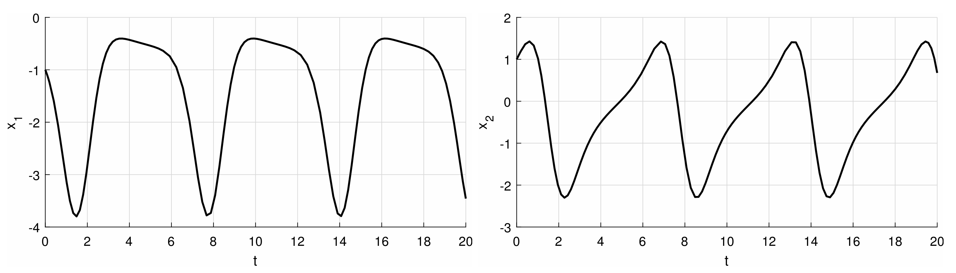
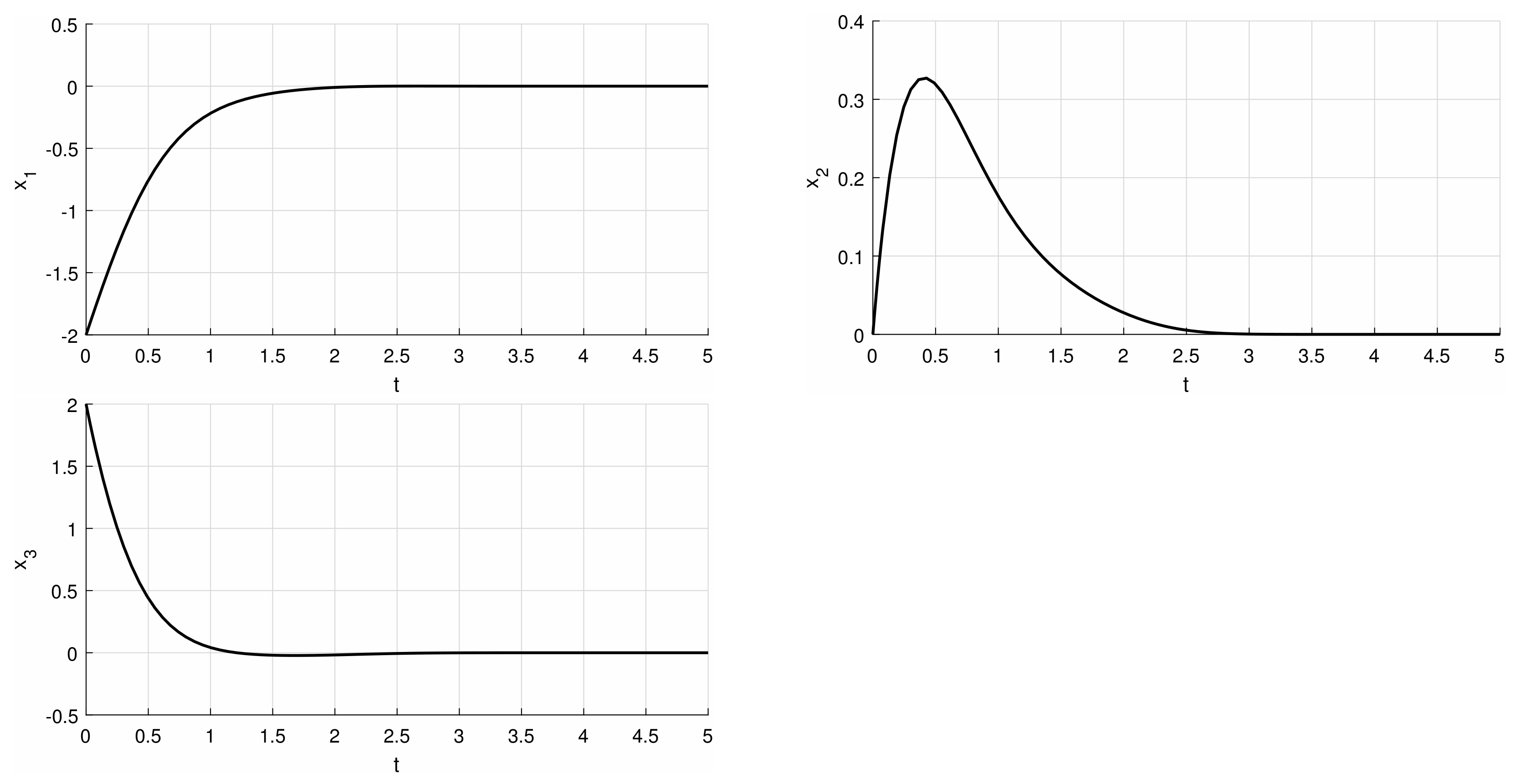
Observation 2. If for every is a normal matrix andwhere is a constant, then the LTV system is UAS. Example 2. Let us consider the LTV system (1),wherewith the spectrum Because the matrix is normal for all (Property 1) and the system is UAS by Observation 2.
Or alternatively, by employing Property 2,for all Thus the estimate (E1) and Lemma 1 also imply uniform asymptotic stability of the system. Moreover, in this specific case when is of the form (here, – in general, could be an arbitrary continuous matrix function), Property 2 implies that and, by the estimate (E2), the modulus of the solution The results of simulation in the MATLAB environment are shown in Figure 1. Example 3. For the LTV system (1) withwhere are continuous functions on the values of the matrix function are in if Proceeding analogously to the previous example, we can observe that For example, if and the system is by Lemma 1 and the estimate (E1) uniformly stable and We will now present the most general statement of this paper, from which Observations 1 and 2 will emerge as special cases. First, let us define some useful concepts and relations between them that will allow us to easily formulate the main result of the paper.
The vector norm
is called
monotonic if
for all
such that
see e.g., [
21]. The notations
(absolute value), and ≤ are to be interpreted componentwise, when applied to vectors. For example, the Euclidean norm
is monotone. Further, if the norm
is monotonic, then
for all diagonal matrices
[
21].
Given
the spectral abscissa is defined as
and
the spectral radius is defined as
The
logarithmic inefficiency [
11,
22] of a vector norm
with respect to the matrix
A is given by
Combining
we find that
and we have the following theorem.
Theorem 4. Let for every is diagonalizable by a nonsingular real matrix and define for all where is a monotonic norm. Then Proof. From
and using that
[
16] we find that
Now, because the similar matrices have the same characteristic polynomial,
and
The property (
6) of a monotonic norm with
and the equality (
7) gives
and so,
for all
which yields (
8). □
Since the estimates (E1) and (E2) hold in general only for the time-invariant vector norm in
(a notable exception are the UAS LTV systems—for details see [
23] (Theorem 3, the inequality (7)) and [
12]), we must impose an additional assumption:
where
is a constant nonsingular real matrix. It is worth noting that we do not have to require the norm
to be monotonic. The monotonic norms
may also differ depending on
The following example documents that this condition may not be omitted.
Example 4. Consider (1) in the vector space endowed with the Euclidean norm and The pointwise eigenvalues are and for all and so the matrix is diagonalizable withand by Theorem 4. But on the other hand, the fundamental matrix solutionshows that in all balls around the origin there is solution arbitrarily near the origin being expelled from a neighborhood of the origin, therefore, the system is unstable. The condition (
9) narrows the class of matrix functions to which we can apply Theorem 4 quite substantially, but as we will now see, the class of normal matrices from Observation 2 is one of them. Indeed, the normal matrices are unitarily diagonalizable, that is,
(for real matrices), for all
Thus, we have for the Euclidean norm in
and for all
in (
9). Theorem 4 then implies
which is in compliance with Corollary 1. For the more general case within the Euclidean norm, when
(obviously,
) from the special form of the eigendecomposition for symmetric positive definite matrices, it follows that
that is,
in (
9) with
and
equal to
.
Observation 3. Let for every is diagonalizable by a nonsingular real matrix and let for all is where are the monotonic norms and is a nonsingular, constant and real matrix.
Ifwhere is a constant, then the LTV system is UAS. 4. Conclusions
In this paper we have established the class of matrix functions
for which the condition
without any additional assumptions constraining the rate of variation in
ensures the uniform asymptotic stability of the LTV system
The main result is formulated in Observation 3. This class consists of the matrix functions with values in the set of normal matrices, the subgroup of which is also an important special orthogonal group
Moreover, for the LTV systems with
for all
we have derived the formula for computing the exact value of vector norm of
The challenge for further research is to find the classes of matrix functions
for which the assumption (
9) applies, that is, for which there is a suitable combination of norms (monotonic norms
and norm
) and a nonsingular constant matrix
similarly to that for matrix functions with values in the set of normal matrices, analyzed just before Observation 3.
The results of this paper could also be an interesting topic for further research regarding control theory as a contribution to the stability theory of linear systems. For example, to design such an adaptive state feedback control law
for the control system
so that the closed-loop system matrix function
satisfies the conditions established in Observation 1, 2 or 3 stabilizing the control system;
in the system matrix function represents the parametric uncertainty. For the last achievements and research directions on the field of stabilizability of the linear control systems, see, for example, Refs. [
24,
25,
26,
27] and the references therein.


