Abstract
The article describes a mathematical model of interconnected electromechanical and thermal processes in a linear induction motor (LIM). Here, we present the structure of the thermal model and provide the calculation formulas of the model. The thermal model consisted of eight control volumes on each tooth pitch of the LIM. Moreover, we also present a model of electromechanical processes and its interaction with the thermal model. The electromechanical model was based on the detailed magnetic and electrical equivalent circuits of the LIM. Model verification was performed using a model based on the finite element method and using experimental data. We also conducted a study focused on the necessity of considering the influence of various features of the thermal processes. We herein discuss the application of the model implemented in the MATLAB/Simulink, which was used to analyze the thermal performance of linear transport and technological induction motors. For the traction single-sided linear induction motor, we determined limits of safe operation by considering the unevenness of heating along the length in two cases: natural cooling and forced cooling. For forced cooling, required values of air flow were determined. For the arc induction motor of the screw press, the influence of various factors (i.e., reduction of the stroke, the use of a soft start, and the use of a forced cooling) on heating was evaluated.
1. Introduction
The analysis of thermal processes in conjunction with electromechanical processes is a priority task in the study of the operating modes of an electric drive based on a linear induction motor (LIM). The need for such analysis may arise when designing a LIM. For example, when designing transport systems with a large field of LIM applications [1], stringent requirements are often imposed on the weight and dimensions of the traction LIMs’ primaries. This entails an increase in magnetic fluxes and current density and, therefore, in overheating primary windings, which lead to the necessity to intensify the cooling.
LIM studies are further complicated by the fact that they significantly differ from the rotating IMs in specific electromagnetic processes due to the longitudinal and transverse edge effects. These phenomena are well examined and described in previous publications [2,3,4,5,6].
Electromagnetic asymmetry along the length of the primary can lead to a significant difference in the distribution of losses along its length and, therefore, to the differences in the thermal processes between the LIM and the rotating IM [7]. This occurrence is common in transport systems when a LIM consists of several primaries and one secondary, which forms an endless conductive plate. In this case, once in motion, the primaries can be in different thermal conditions because the conductive plate gradually heats up while passing through the zone of each primary. Therefore, a phenomenon of the heat transfer from the primary through the air gap takes place. In the LIM technological applications, the secondary is often a part of an actuating element of the technological machine, which also leads to heat transfer specifics.
The circumstances listed above complicate the use of techniques, described, for example, in [8], and are traditionally used for rotating electric machines based on simple thermal equivalent circuit models with from 1 to 4 nodes. In [9], there is a detailed thermal equivalent circuit of a low-power induction motor containing 107 nodes (thermal masses). In [10], the analysis of the development and current state in the field of thermal processes analysis in electric machines is presented. Studies [9,10], as well as many others [11,12,13,14,15], are devoted to calculating the thermal performance and cooling system performance of rotating electric motors, which, as mentioned above, have significant differences from linear electric motors in both design and physical processes. However, the results obtained by analyzing heat transfer in rotating electric motors are, in some cases, also applicable to linear electric motors—e.g., in the patterns of convective heat transfer of the winding front parts [16]; in the determination of the equivalent thermal conductivity of the winding [17]; and in the determination of other parameters that critically impact heat transfer [18].
Other studies [19,20] have examined thermal processes in synchronous tubular linear electric motors that differ in principles of operation from induction motors. One such study [21] considered a computationally efficient approach for calculating the thermal performance of permanent-magnet synchronous linear motors using a 3-D thermal equivalent circuit. In another study [22], the authors describe an analytical model that combines electrical and thermal approaches for a canned rotating induction motor. Another set of studies [23,24,25] have been devoted to the thermal modelling, design, and analysis of linear motors (induction and synchronous).
A similar approach based on equivalent circuits (lumped-parameter models) is widespread in LIM studies [26,27,28,29,30,31,32,33,34] for the calculation of electromagnetic and electromechanical processes. In aforementioned studies the following detailing levels are considered: electrical equivalent windings’ circuits, down to a winding section or phase, or magnetic, down to a tooth pitch.
The development of models that consider the coupled thermal and electromechanical processes specifically for the LIM remains relevant. The main goal of this study was to develop a tool that allows for the analysis and design of a LIM which considers peculiarities within the interconnected electromechanical and thermal processes.
2. Thermal Model
The thermal model considers the following features:
- heat (mass) transfer from the air gap during movement;
- non-uniform longitudinal distribution of losses due to the longitudinal edge effect and non-uniform longitudinal heating;
- losses in the secondary outside of the air gap in the longitudinal direction;
- losses in the magnetic cores;
- influence of the temperatures of LIM parts on the electromechanical characteristics and losses;
- thermal conductivity between LIM parts;
- heat transfer by radiation with the environment between the primary and secondary;
- heat transfer from the LIMs external surfaces, taking into account the conditions of natural convection or forced convection;
- equivalent slot and front parts of the primary winding thermal conductivity in different directions, taking into account the thermal conductivity of insulation;
- thermal conductivity dependence on temperature.
It is possible to detail the model down to the tooth pitch level, pole pitch, several pole pitches, and the full length of the primary. Detailing is dictated by the calculation task. In this study, we assumed a detailing level that could detail down to tooth pitch. For each tooth pitch, eight control volumes (thermal masses) were considered [35]:
- slot part of winding (equivalent material, taking into account the ratio of volumes of conductors and slot insulation according to recommendations [15]);
- part of the magnetic core above the slot;
- part of the magnetic core above the tooth;
- the tooth;
- front part of winding on the ‘left’;
- front part of winding on the ‘right’;
- secondary conductive plate;
- secondary magnetic core (iron plate).
The thermal model is shown in Figure 1 and Figure 2, where qr are heat fluxes due to radiation; qv are heat fluxes due to mass transfer caused by the movement of the primary or secondary; qt are heat fluxes of thermal conductivity; and qc are heat fluxes of convection.
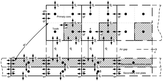
Figure 1.
Thermal model of the LIM—longitudinal section.
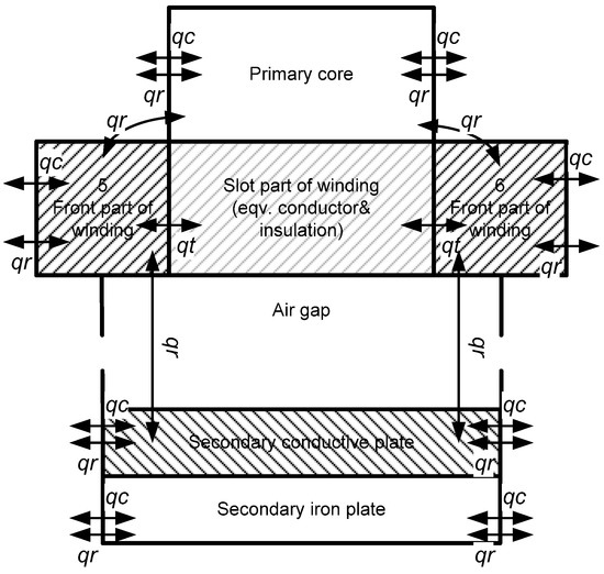
Figure 2.
Thermal model of the LIM—cross section.
In general, the heat equation in the case of mass transfer along the x axis is as follows [36]:
where a is the temperature conductivity [m2/s]; Q is the power density of heat source [W/m3]; c is the specific heat capacity [J/(kg°C)]; is the density [kg/m3]; T is the temperature [°C]; and v is the speed, [m/s].
The finite-difference approximation for Equation (1) is performed using the second derivative approximation on the coordinate according to Equation (2). To approximate the first derivative on the coordinate in [36,37], the upstream-difference scheme is recommended for calculation of mass transfer processes as the most stable; therefore, Equation (3) is used. In Equations (2) and (3), h is the step [m] along the x coordinate.
The solution of Equation (1), obtained using Laplace transform, can be written as Equation (4):
In Equation (4), and are thermal conductivity heat fluxes between adjacent control volumes [W]; and are equivalent heat fluxes that describe mass transfer between the adjacent control volumes [W]; is the heat flow due to heat generation in the i-th control volume [W]; is the mass of the i-th control volume [kg]; is the specific heat capacity of the i-th control volume; and p is the Laplace operator.
Heat fluxes of thermal conductivity in (4) are determined according to Equation (5).
In Equation (5), is the thermal conductivity coefficient [W/(m·°C)]; is the contact surface area between the adjacent control volumes [m2]; and is the distance between the centers of the adjacent control volumes of the thermal equivalent circuit [m].
To calculate the heat flux of thermal conductivity between bodies with different coefficients of thermal conductivity, it is necessary to apply thermal conductivity that is averaged at the boundary. According to [36], it is recommended to use the harmonic mean rather than the arithmetic mean, especially when there are significant differences in the coefficients. When performing the averaging, the geometric dimensions of each control volume must be considered [36]. Thus, for a composite body with a layer boundary located between two points, the expression for the coefficient of thermal conductivity through the boundary between the control volumes is as follows [36]:
In Equation (6), are the thermal conductivity coefficients of the adjacent control volumes; and are the lengths in the direction of heat transfer of the adjacent control volumes.
The thermal conductivity coefficient of each control volume was determined as follows:
In Equation (7), A and B are reference coefficients for heat-conducting materials.
Equivalent heat fluxes from a mass transfer were calculated according to Equations (8) and (9):
Radiation heat fluxes (10) and convection heat fluxes (11) along other coordinates according to the heat flux distribution scheme in Figure 1 and Figure 2 are also added as summands to Equation (4).
In the Equation (10), are relative emissivity of the surfaces of the control volumes involved in the heat transfer by radiation; is the area of mutual exposure [m2].
In Equation (11), is the convection coefficient of the surface of the i-th control volume [W/(m2·°C)]; is the surface area of the i-th control volume [m2]; and is the ambient or coolant temperature [°C].
To determine the conditions of convective heat transfer for special types of the LIM, a hydraulic calculation of the forced cooling system is required. The hydraulic calculation consists of determining the hydraulic resistance of the cooling system according to previous recommendations [38], pressure losses along the path from inlet to the outlet of cooling system, and the coolant speeds in the channels.
The example of the calculation procedure and its result for the traction LIM of an urban transportation system was described in detail for the first time in [39]. The convection heat transfer processes [40,41,42], in turn, depends on the various speeds of the coolant in channels. Convection processes were calculated using the theory of similarity based on Reynolds, Euler, Prandtl, Grashof, Nusselt, and Peclet criterions (numbers) [40,41,42]. Recommendations [15] were used to describe the convective heat transfer of the front parts of the winding. Simulink models of the convective heat transfer are described in detail in [43].
3. Influence of the LIM Parts Temperatures on Electromechanical Processes
The losses in windings and magnetic cores, which are necessary for temperature calculation as heat sources, as well as the speed of the LIM movable part in a considered mode, are determined by a calculation according to the electromechanical model based on detailed magnetic and electrical equivalent circuits, as described in [26,27]. The electromechanical model is based on Equation (12).
where U is the supply line-line voltage vector [V]; is the impedance matrix of the primary phases (Ohm), is the resistance matrix (Ohm); is the self-inductance matrix (H); ω is the angular frequency, ω = 2πf, where f is the power supply frequency (Hz); is the primary phase current vector (A); w is the number of the turns in slots; is the conversion matrix of the slot electromotive forces (EMF) to the phase EMFs; Φ1, Φ2 are magnetic flux vectors of the primary core and secondary core (Wb); are the reluctance matrices (AT/Wb); is the conversion matrix of phase currents to the slot currents; is the secondary conductive plate current vector (A); is the secondary impedance matrix (Ohm); is the secondary conductive plate EMF matrix [V]; is the traction force (N), ; is the load force (N); M is the mass of the LIM movable part (kg); and v is the speed of the LIM movable part (m/s).
In interconnected models of electromechanical and thermal processes, the influence of the LIM parts temperatures on electromechanical characteristics and on the losses is considered according to the approach described in [7,35]. In general, the dependences f1, f2, and f3 of the traction force and losses in the selected control volumes of the primary winding and of the secondary conductive plate are described as (13). In Equation (13), N is the number of primary winding control volumes in the thermal model; K is the number of secondary conductive plate control volumes in the thermal model; is the temperature of the primary winding control volumes; and is the temperature of the secondary conductive plate control volumes.
Figure 3 shows the submodels interconnection scheme of the LIM model [7] where is the speed setpoint; is the coolant speed at the outlet of the discharge device (pump or fan); are the coolant speeds in the cooling channels; is the loss vector in primary control volumes, including winding and magnetic core; is the secondary control volumes loss vector, including conductive plate and magnetic core; is the primary control volumes temperature vector, including winding and magnetic core; and is the secondary control volumes temperature vector, including conductive plate and magnetic core.
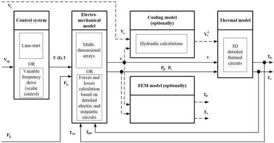
Figure 3.
Submodels interconnection scheme.
As a rule, the time constants of thermal transients are multiple times greater than the time constants of the mechanical transients, which in turn are times greater than the time constants of the electromagnetic transients. While studying thermal transients, to reduce the calculation time, it is advisable to avoid directly combining different submodels into a single master model that describe processes of different time scales, which leads to stiff differential equations systems, the need to use special solvers, and a huge calculation time for the thermal processes.
Therefore, the electromechanical model of each studied LIM was presented in the form of a multidimensional array, which is filled in advance by calculation using the original model. The dimensions of the array are slip, power supply frequency, primary winding temperature, and the secondary conductive plate temperature. The output value is traction force. In this case, slip is a function of the load force and the power supply frequency. It is possible to include voltage dimension in the array (in case of taking into account the saturation of magnetic cores). Similar arrays were used to determine the losses in the primary winding and the secondary conductive plate. This approach accelerates calculations up to 10 times because sampling a value from a pre-filled array using multidimensional interpolation is much faster than using an electromechanical model for direct calculation.
The arrays used for the traction LIM of the urban transportation system calculations are presented in Table 1. The variables ranges are: slip: 0–1 relative units (r. u.); frequency: 5–40 Hz; secondary conductive plate temperature: 0–200 °C; primary winding temperature: 0–200 °C. Detailed recommendations on the step values of filling the array for each coordinate and the choice of interpolation algorithms are described in [35].

Table 1.
An example of multidimension arrays.
Implementation of the electromechanical and thermal models in the MATLAB/Simulink based on the aforementioned equations and multidimensional arrays described in detail in [44].
4. Experimental Verification of the Model
A comparison of the thermal processes calculation results of the LIM experimental unit (Figure 4) was performed with experimental data. The LIM consists of two primary cores in opposite slots of which ring coils are installed with phasing +A − C + B − A + C − B + A − C + B along the length. In the gap between the cores, there is an aluminum plate and solid back iron. The main parameters of the LIM are given in Table 2.
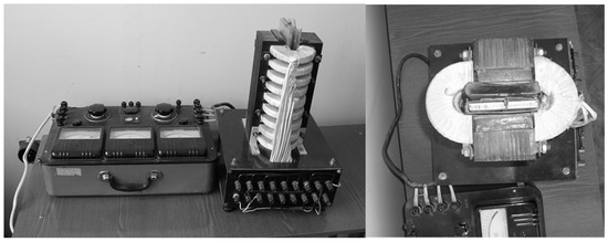
Figure 4.
The LIM experimental unit.
Table 2.
Parameters of the LIM experimental unit.
During the experiments on this unit, the average temperature of the secondary conductive plate was determined. Figure 5 shows the calculation results and the experimental results at zero speed. The experimental value at time t = 60 s was excluded from further analysis. The maximum absolute error of the calculation does not exceed 2 °C; the maximum relative error does not exceed 3%. The root-mean-square (RMS) error is 1.2%.
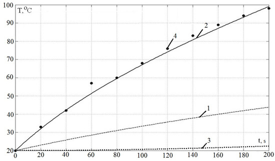
Figure 5.
Comparison of calculation results and experiment. 1—primary winding average temperature (calculated); 2—secondary conductive plate average temperature (calculated); 3—primary core average temperature (calculated); 4—secondary conductive plate average temperature (experiment).
5. Finite Element Method Verification of the Model
The results of the calculation of the thermal processes of the experimental LIM based on the three-phase primary SL-5-100 (Figure 6 and Table 3) are compared with the calculation according to the model based on the finite element method (FEM). The assumptions of the FEM model partially coincide with the assumptions of the developed thermal model: the equivalent winding material was specified; losses were calculated using the same electromagnetic model; the coefficient of thermal conductivity dependence on temperature was considered. Figure 7 shows the 2D geometrical model and the results of calculating the temperature and heat fluxes for zero speed in a two-dimensional formulation (for time t = 1250 s). The calculation results of the thermal transient are shown in Figure 8.
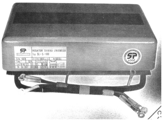
Figure 6.
Primary SL-5-100.
Table 3.
Parameters of the LIM based on SL-5-100.
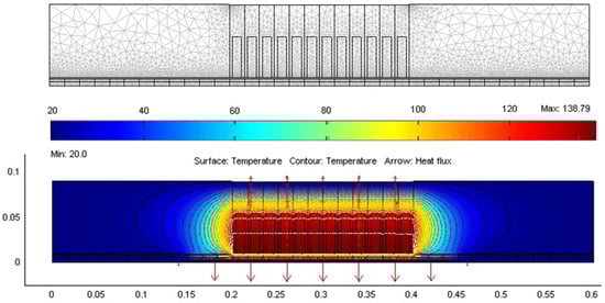
Figure 7.
The results of thermal calculation according to the FEM model.
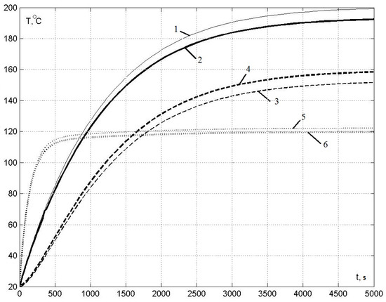
Figure 8.
Comparison of calculation results with the FEM model. 1—primary winding average temperature; 2—primary winding average temperature (FEM); 3—primary magnetic core average temperature; 4—primary magnetic core average temperature (FEM); 5—secondary conductive plate average temperature; 6—secondary conductive plate average temperature (FEM).
The average temperature of the slot part of the winding, the average temperature of the primary magnetic core, and the average temperature of the conductive plate of the secondary were compared. The greatest differences in the calculation results were observed in the temperatures of the slot part of the winding. For steady-state thermal conditions:
- The maximum absolute error in calculating the temperature of the slot part of the winding does not exceed 8 °C; the maximum relative error does not exceed 4.2%.
- The maximum absolute error in calculating the temperature of the secondary conductive plate is no more than 2 °C; the maximum relative error is no more than 1.7%.
- The maximum absolute error in calculating the temperature of the primary magnetic core is no more than 8 °C; the maximum relative error is no more than 5%.
Moreover, the FEM verification was conducted for the traction LIM of the urban transportation system and demonstrated the error within 3.8–4.8%. It is described in more detail in [44].
6. Model Experiments
Over the course of the model experiments, the goal was to assess the influence of various factors on the thermal performance of the LIM. As a result, recommendations were developed in order to consider the specifics of the thermal processes in the LIMs, which were used in the analysis of the real LIM. Therefore, using the experimental LIM model based on the SL-5-100 primary, the effects on the calculation result of a number of factors and phenomena were investigated [35]. The initial and ambient temperatures are assumed to be 20 °C in all calculations.
6.1. Effect of the Speed on the Thermal Condition of the LIM
At the speed of more than 0.01 m/s, the temperatures of the secondary averaged over length can be considered, since the heating of the secondary during the moving time under the primary is insignificant (less than 1 °C) and the temperatures in the neighboring areas differ little from each other. When stopping (short circuit mode), the temperature reaches about 120 °C, and there is uneven temperature distribution between the areas under the primary and beyond. In general, for the secondary, heat transfer fluxes caused by mass transfer prevail even at speeds of more than 0.005 m/s. For example, when setting in the model experiment the temperature 200 °C as a boundary condition for areas of the secondary entering the primary, a gradual decrease in temperature is observed only to 130 °C in the interval equal to 3 lengths of the primary.
6.2. Temperature Distribution on the Tooth Pitch and Along the Length of the LIM Primary
The following operation mode was set for the frequency adjustment (linear scalar control U/f = const): low load (speed setpoint 0.7 m/s, U = 30 V, f = 7 Hz, load force 5 N), then increase speed setpoint up to 3 m/s at t = 5000 s (U = 132 V, f = 30 Hz), then increasing the speed setpoint to 5 m/s at t = 10,000 s (U = 220 V, f = 50 Hz), then a load increases up to 110 N at t = 15,000 s, then a load decreases to the initial value of 5 N (at t = 25,000 s).
Figure 9 and Figure 10 show the results of the calculation of these modes. The additional heating is discovered due to the increase in losses when increasing the speed setpoint (i.e., voltage and frequency) or during the increase of the load. However, when switching to a speed of 5 m/s, cooling takes place because the losses increase insignificantly, and the heat transfer from the LIM surfaces is significantly improved because of a non-linearly dependency of the convection coefficients on speed. Moreover, a quick cooling occurs when the load decreases because of the speed, and hence, the intensity of the convection processes, remains high, and electrical losses proportional to the square of the current are sharply reduced.
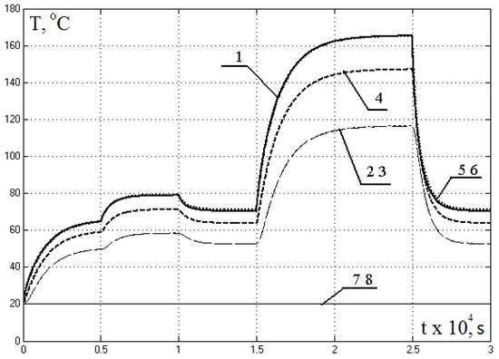
Figure 9.
Temperatures on the 6-th tooth pitch: 1—slot part of primary winding; 2—primary magnetic core part above slot; 3—primary magnetic core part above tooth; 4—tooth; 5, 6—front parts of primary winding; 7—secondary conductive plate; 8—secondary magnetic core.
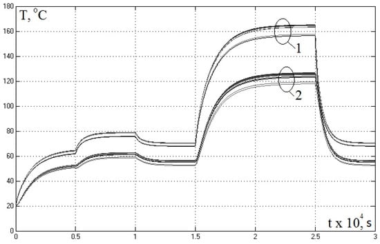
Figure 10.
Average temperatures along primary length. Curve group 1—primary winding on tooth pitches; curve group 2—magnetic core on tooth pitches.
According to the graphs in Figure 9, the most heated element is the winding. The temperature of the slot part is in only by 1% more than the temperatures of the front parts. The tooth is the most heated section of the magnetic core, its temperature is about by 11–13% less than that of the slot part of the winding. The temperatures of the yoke parts are 20–25% less than the temperature of the tooth.
In Figure 10, the average temperature of the primary winding on the tooth pitches is the average value between the temperature of the slot part of the winding and the temperatures of the front parts. The average temperature of the primary magnetic core on the tooth pitch is the average value between the temperatures of two parts of the magnetic core (above the slot and above the tooth) and the temperature of the tooth.
Figure 10 shows the following patterns. Along the length of the primary, the temperatures of the winding and the magnetic core almost do not change, except for the two edge zones (two lower curves in each group of curves in Figure 10). The maximum difference in the most intensive mode is 7 °C, and in other modes, the difference is about 3.0–4.5% in average. This allows in many cases to consider the temperature of the primary winding and the magnetic core averaged over the primary length. However, for some LIMs, this assumption might be not correct.
6.3. Accounting of the Non-Linear Thermal Conductivity
In models that do and do not account for the nonlinear dependence of the thermal conductivity coefficient on temperature, the start-up and operation under a rated load were investigated due to the significant heating in this mode. The temperature curves of the secondary do not differ from each other for the two cases considered, because the cold parts of the secondary constantly come under the primary and during the movement under the primary do not have time to significantly heat up. Thus, the secondary temperature is almost equal to the ambient temperature, therefore, the thermal conductivity coefficient does not vary. The temperature difference in transients for the primary with and without considering non-linear thermal conductivity is about 1–2 °C. Thus, it is not mandatory but desirable to take into account the dependence of thermal conductivity coefficients on temperature because it allows a slight increase in the accuracy of the simulation.
6.4. Accounting Radiation
The start-up under the rated load is considered because it leads to the significant heating. The transients were compared with and without radiation. The temperature was averaged over the length of the LIM. Lack of accounting for radiation leads to the overestimated temperature of the primary in the model, so for the steady-state values of the temperature of the primary winding, the excess is about 30 °C, i.e., by 25%. Such significant differences occur due to the fact that at a temperature of about 120 °C a significant fraction of the heat is transferred to the environment and to the slightly heated secondary, which significantly affects the processes. Thus, it is necessary to account for the radiation processes in the thermal LIM model, especially at temperatures of the LIM parts above 100 °C.
6.5. Accounting for Forced Convection
A direct start-up at the rated load was considered, then after the end of the thermal transient the load was set to 10 N in order to compare modes at low speed and at high, close to synchronous, speed. The transients were compared when taking into account the variations in heat transfer coefficients with a change in the speed—in this case, a heat transfer coefficient corresponding to the natural convection was used in calculations, depending only on the surface temperature and not depending on the air flow speed. According to the results, it can be concluded that the lack of account for the forced convection leads to the excessive heating of the primary in the model. This is due to the fact that the natural convection coefficients are in this case 3–5 times less than the forced convection coefficients, especially at high speeds. For the primary in the first mode (at the rated load), the difference in steady-state values of the winding temperature is about 60 °C (about 50%). For the second mode (at a reduced load and high speed), the difference is even greater and is about 90 °C (about 130%). Thus, the calculation of the heat transfer coefficients based on the criteria equations of the forced convection is necessary.
In a multi-primary drive, in transport applications, a situation is possible that a stagnant air forms under the last primaries even at high speeds of the train. Thus, the abovementioned findings also allow to estimate the difference in thermal conditions of the first and last primaries.
6.6. Accounting for Losses in the Magnetic Core of the Primary
The following mode was considered: start-up at low load 10 N with a speed setpoint of 5 m/s, then load rapidly increases up to rated load. Transients were compared with and without considering losses in magnetic cores; it showed difference less than 0.1 °C. The losses in the primary core for IM are quite small in comparison with the losses in the winding and occur in the magnetic core, which has a much better cooling conditions than the winding, especially its slot part. Therefore, for the considered LIM construction, magnetic losses calculation is not mandatory. However, in the case of the LIM with a solid secondary without a conductive layer, their share, as a rule, is much larger and it is undesirable to neglect losses in solid cores.
7. Practical Results
Using the described mathematical model and the MATLAB/Simulink programs created on its basis, the traction LIM of the urban transportation system and the arc LIM of the screw stamping press and several other LIM were calculated.
7.1. Traction Single-Sided LIM for the Urban Transportation System
The primary of the traction single-sided LIM for the urban transportation system is shown in Figure 11. The LIM operates as a part of a variable speed drive. The main parameters of the LIM are given in Table 4. The design features of the LIM and the configuration of its cooling system were taken into account during calculation. Detailed results of the hydraulic calculation of the cooling system are given in [39] and were adopted for the current study.
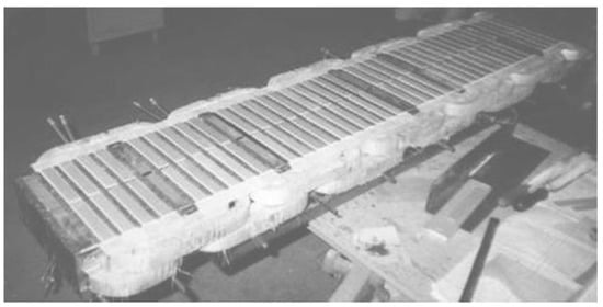
Figure 11.
The traction LIM primary at the winding installation stage.
Table 4.
Parameters of the traction LIM of the urban transportation system.
- For typical operating modes, the unevenness of heating along the length of the traction primary LIM is studied. It was found that the temperature of the winding at different tooth pitches can vary in the transient up to 1.3–1.8 times due to the specifics of the winding [7].
- The secondary conductive plate heating was investigated at a soft start (assuming linear scalar control 5–38 Hz and ramp-up time 20 s) to a speed of 50 km/h with a low load of 1850 N and natural cooling. Figure 12 shows the calculation result. In the Figure 12, the peak value of the secondary conductive plate temperature is about 37 °C under a single primary. For the direct start-up under the same conditions, the peak value of the heating of the conductive plate of the secondary is about 68 °C. In the case of start-up at full load of 8000 N, the peak value of the heating of the conductive plate of the secondary under single primary at a soft start is about 75 °C, and with a direct start-up—about 123 °C.
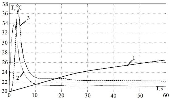 Figure 12. Average temperatures of the traction LIM during soft start. 1—primary winding; 2—secondary conductive plate (area under the primary); 3—secondary conductive plate near the exit end of the primary (area outside the primary).
 - The effect of the heating of the secondary by the previous primaries on the heating of the winding of the selected primary takes place in a multi-primary drive of the train consisting of several carriages, each of which has its own primary. In the model experiment, the pre-heated to 100 °C secondary entering under the primary was considered. Table 5 shows the results of calculating the additional heating of the primary winding (ΔT) at various speeds.
Table 5. Dependence of additional heating of primary winding on train speed with a preheated secondary.
For the traction LIM, the limits of a safe operation (RMS values of primary phase currents) are determined by considering the unevenness of the heating along the length in the cases of natural and forced cooling systems, as well as of different air flows in the forced cooling system. Recommendations for the air flow rate have been previously formulated [7]. The obtained results are shown in Table 6 and Table 7:
Table 6.
Maximum steady-state primary winding temperatures during natural cooling.
Table 7.
Maximum steady-state temperatures of primary winding during forced cooling.
- 4.
- In the case of natural cooling (Table 6), operation at the current of more than 135 A is impossible because it leads to an increase in the primary winding temperature above 180 °C. This corresponds to the start-up load limit of 1850 N which is typical for an empty train. With increasing frequency, the heating at the same current decreases, because the speed of the train increases and the cooling of the primaries improves.
- 5.
- The traction LIM operation at the maximum load (current 270 A, load force 8000 N) is possible in the case of forced cooling at a flow rate of cooling air of at least 2.2 m3/s (Table 7).
The described features of thermal processes in the traction LIM and the need for the forced cooling result from its limited size in width (240 mm) and height (110 mm), which entailed the use of a special winding with a minimum length of the front parts, which also contributes to the uneven heating along the length of the primary.
7.2. Screw Press Arc Induction Motor
The thermal performance of the screw press arc induction motor (arc IM) was estimated (Figure 13). The main parameters of the arc LIM are given in Table 8. Two arc stators are located on the top plate of the press, one opposite the other (Figure 14). A steel flywheel is situated between arc stators. The flywheel is a solid steel secondary (rotor), without separated conductive and magnetic layers. The flywheel is connected to a screw, which through the screw-nut gear provides a linear movement of the punch. The rated stamping force is 2500 kN. It is determined by the kinetic energy of the rotating flywheel.
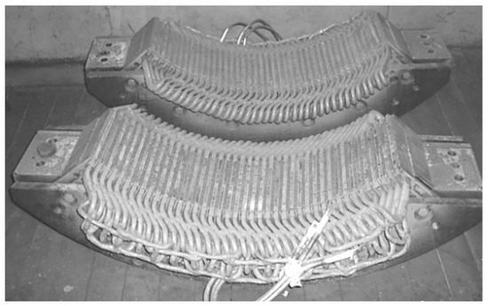
Figure 13.
Arc stators of the screw press arc IM before mounting.
Table 8.
Parameters of the screw press arc IM.
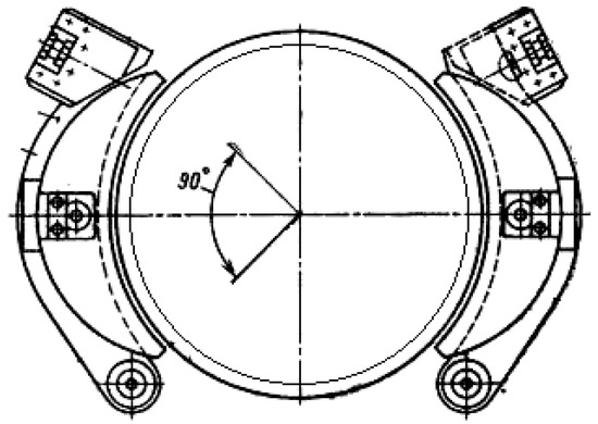
Figure 14.
Position of the arc stators relative to the secondary flywheel.
The task was to improve the press productivity. With an expected productivity of 30 strokes/min with a stroke length of 400 mm, the operation cycle assumed as follows: 0.6 s—downward stroke with the motor turned on; 0.25 s—downward stroke running-out and hit; 0.3 s—upward stroke with the motor turned on; 0.5 s—upward stroke running-out; 0.35 s—braking and pause.
According to the results of the screw press arc IM calculations, the influence of various factors on heating was evaluated: reduction of the stroke (duration of switching on state), the use of a soft start (gradually increasing voltage), and the use of forced cooling. As a result of the studies of the arc IM, the following conclusions were formulated:
- In all operating modes, the temperatures of the secondary around the circumference are approximately the same. Similarly, the temperatures of the stator windings on different tooth pitches are approximately the same. Therefore, for analysis, it is possible to use temperatures averaged over the circular length of the secondary and over the stator.
- The flywheel rotor (secondary) heats up about five times faster than the primary winding due to the heat transfer conditions and the presence of significant losses in solid iron.
- A comparison of the calculation results and operational data for the rated operating mode of the press during a direct start-up and forced cooling of the arc IM are presented in Table 9 and demonstrate good calculation accuracy. The scatter of experimental data in Table 9 took place due to the ambient temperature variations in an industrial enterprise and other factors.
Table 9. Comparison of experimental and calculated temperatures arc IM for rated operation with direct start-up.
- In the absence of forced cooling during the rated cycle time of 2 s, an unacceptable overheating of the stator windings occurred, both during direct start-up (after approximately 58 min or 1730 cycles) and during the soft start (after approximately 68 min or 2050 cycles). To ensure the planned performance of the press, forced cooling is required with an air flow rate of at least 6 m3/s, which corresponds to a fan power of at least 4 kW. In the case of natural cooling, a pause after each cycle of at least 4 s is necessary.
- Losses at the soft start are approximately 10% less than at the direct start. Accordingly, the heating of the stator windings becomes 8.1% less already at the time of the voltage ramp-up to the nominal value equal to 2 periods of the mains. The heating of the secondary surface layer becomes 13.5% less. A further increase in the voltage ramp-up time does not lead to a significant reduction in losses and, accordingly, heating. The calculation results of thermal processes for the case of soft start with forced cooling at a nominal cycle time are shown in Figure 15.
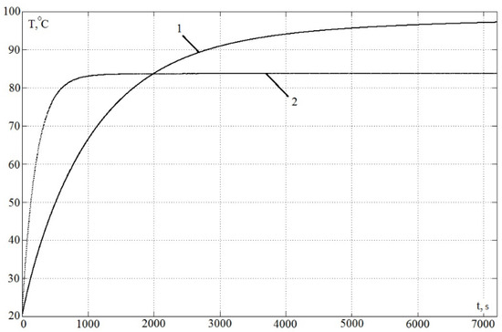 Figure 15. Average temperatures of the arc LIM during soft start. 1—stator winding; 2—secondary surface layer.
8. Conclusions
As a result of the work performed, a mathematical model of the interconnected electromechanical and thermal processes in the linear induction motors was created. A computationally efficient approach based on multidimensional arrays was used for thermal processes calculation. The model was implemented in MATLAB/Simulink. The experimental verification of the calculation results was carried out, as was the verification using FEM models. An assessment of the influence of various factors on the thermal performance of the LIM was performed. As a result, the recommendations to consider a number of peculiarities of thermal processes in the LIMs were formulated, which were used in the analysis of a real LIM. The analysis of the thermal performance of the LIM of various designs for the transport and technological applications was performed. The main results are as follows:
- for the traction single-sided linear induction motor, limits of safe operation are determined when taking into account the unevenness of heating along the length for natural and forced cooling, in which required values of airflow in the forced cooling system were determined;
- for the screw press arc induction motor, the influence of various factors on heating was evaluated, i.e., reduction of the stroke, the use of a soft start, and the use of forced cooling.
Author Contributions
Conceptual approach, F.S. and V.G.; data curation, V.P. and V.G.; calculations and modeling, V.G. and V.D.; writing of original draft, V.G., V.D. and V.P.; visualization, V.G. and V.P.; review and editing, V.D., F.S. and V.P. All authors have read and agreed to the published version of the manuscript.
Funding
The work was partially supported by the Ministry of Science and Higher Education of the Russian Federation (through the basic part of the government mandate, Project No. FEUZ 2020-0060).
Institutional Review Board Statement
Not applicable.
Informed Consent Statement
Not applicable.
Data Availability Statement
The manufacturers’ technical specifications of the linear induction motors were used for the analysis.
Acknowledgments
The first author would like to express his profound gratitude to his recently passed away mother for supporting him on the long way of electrical engineer and researcher.
Conflicts of Interest
The authors declare no conflict of interest. The funders had no role in the design of the study; in the collection, analyses, or interpretation of data; in the writing of the manuscript; or in the decision to publish the results.
References
- Palka, R.; Woronowicz, K. Linear induction motors in transportation systems. Energies 2021, 14, 2549. [Google Scholar] [CrossRef]
- Boldea, I. Linear Electric Machines, Drives, and MAGLEVs Handbook; CRC Press: Boca Raton, FL, USA, 2013. [Google Scholar]
- Yamamura, S. Theory of Linear Induction Motors; Halsted: New York, NY, USA, 1979; Volume 1. [Google Scholar]
- Gieras, J.F. Linear Induction Drives; Oxford University Press: London, UK, 1994. [Google Scholar]
- Laithwaite, E.; Barwell, F. Application of linear induction motors to high-speed transport systems. Proc. Inst. Electr. Eng. 1969, 116, 713–724. [Google Scholar] [CrossRef]
- Bolton, H. Transverse Edge Effect in sheet-rotor induction motors. Proc. Inst. Electr. Eng. 1969, 116, 725–731. [Google Scholar] [CrossRef]
- Sarapulov, F.N.; Goman, V.V. Development of mathematical models of thermal processes in linear asynchronous motors. Russ. Electr. Eng. 2009, 80, 431–435. [Google Scholar] [CrossRef]
- Anuchin, A.S.; Fedorova, K.G. A Two-mass thermal model of the induction motor. Russ. Electr. Eng. 2014, 85, 83–86. [Google Scholar] [CrossRef]
- Kylander, G. Thermal Modelling of Small Cage Induction Motors. Ph.D. Thesis, Chalmers University of Technology, Gothenburg, Sweden, 1995. [Google Scholar]
- Boglietti, A.; Cavagnino, A.; Staton, D.; Shanel, M.; Mueller, M.; Mejuto, C. Evolution and modern approaches for thermal analysis of electrical machines. IEEE Trans. Ind. Electron. 2009, 56, 871–882. [Google Scholar] [CrossRef] [Green Version]
- Staton, D.A.; Cavagnino, A. Convection heat transfer and flow calculations suitable for electric machines thermal models. IEEE Trans. Ind. Electron. 2008, 55, 3509–3516. [Google Scholar] [CrossRef] [Green Version]
- Alberti, L.; Bianchi, N. A coupled thermal-electromagnetic analysis for a rapid and accurate prediction of IM performance. IEEE Trans. Ind. Electron. 2008, 55, 3575–3582. [Google Scholar] [CrossRef]
- Traxler-Samek, G.; Zickermann, R.; Schwery, A. Cooling airflow, losses, temperatures in large air-cooled synchronous machines. IEEE Trans. Ind. Electron. 2010, 57, 172–180. [Google Scholar] [CrossRef]
- Weili, L.; Chunwei, G.; Ping, Z. Calculation of a complex 3-D model of a turbogenerator with end region regarding electrical losses, cooling, heating. IEEE Trans. Energy Convers. 2011, 26, 1073–1080. [Google Scholar] [CrossRef]
- Borisenko, A.I.; Yakovlev, A.I. Aerodynamics and Heat Transfer in Electric Machines; Energy: Moscow, Russia, 1974. (In Russian) [Google Scholar]
- Madonna, V.; Walker, A.; Giangrande, P.; Serra, G.; Gerada, C.; Galea, M. Improved Thermal Management and Analysis for Stator End-Windings of Electrical Machines. IEEE Trans. Ind. Electron. 2019, 66, 5057–5069. [Google Scholar] [CrossRef]
- Boglietti, A.; Carpaneto, E.; Cossale, M.; Vaschetto, S.; Popescu, M.; Staton, D. Stator winding thermal conductivity evaluation: An industrial production assessment. In Proceedings of the 2015 IEEE Energy Conversion Congress and Exposition (ECCE), Montreal, QC, Canada, 20–24 September 2015. [Google Scholar] [CrossRef]
- Boglietti, A.; Cavagnino, A.; Staton, D. Determination of Critical Parameters in Electrical Machine Thermal Models. IEEE Trans. Ind. Appl. 2008, 44, 1150–1159. [Google Scholar] [CrossRef]
- Huang, X.; Li, L.; Zhou, B.; Zhang, C.; Zhang, Z. Temperature calculation for tubular linear motor by the combination of thermal circuit and temperature field method considering the linear motion of air gap. IEEE Trans. Ind. Electron. 2014, 61, 3923–3931. [Google Scholar] [CrossRef]
- Vese, I.; Marignetti, F.; Radulescu, M.M. Multiphysics approach to numerical modeling of a permanent-magnet tubular linear motor. IEEE Trans. Ind. Electron. 2010, 57, 320–326. [Google Scholar] [CrossRef]
- Tessarolo, A.; Bruzzese, C. Computationally efficient thermal analysis of a low-speed high-thrust linear electric actuator with a three-dimensional thermal network approach. IEEE Trans. Ind. Electron. 2015, 62, 1410–1420. [Google Scholar] [CrossRef]
- Tinni, A.; Knittel, D.; Nouari, M.; Sturtzer, G. Electrical–thermal modeling of a double-canned induction motor for electrical performance analysis and motor lifetime determination. Electr. Eng. 2021, 103, 103–114. [Google Scholar] [CrossRef]
- Nituca, C.; Chiriac, G.; Cuciureanu, D.; Dumitrescu, C.; Zhang, G.; Han, D.; Plesca, A. Thermal modeling of a linear induction motor used to drive a power supply system for an electric locomotive. Therm. Sci. 2019, 23, 589–597. [Google Scholar] [CrossRef]
- Bertola, L.; Cox, T.; Wheeler, P.; Garvey, S.; Morvan, H. Thermal design of linear induction and synchronous motors for electromagnetic launch of civil aircraft. IEEE Trans. Plasma Sci. 2017, 45, 1146–1153. [Google Scholar] [CrossRef]
- Eguren, I.; Almandoz, G.; Egea, A.; Elorza, L.; Urdangarin, A. Development of a thermal analysis tool for linear machines. Appl. Sci. 2021, 11, 5818. [Google Scholar] [CrossRef]
- Dmitrievskii, V.; Goman, V.; Sarapulov, F.; Prakht, V.; Sarapulov, S. Choice of a numerical differentiation formula in detailed equivalent circuits models of linear induction motors. In Proceedings of the 2016 International Symposium on Power Electronics, Electrical Drives, Automation and Motion (SPEEDAM), Capri, Italy, 22–24 June 2016. [Google Scholar] [CrossRef]
- Sarapulov, F.N.; Frizen, V.E.; Shvydkiy, E.L.; Smol’yanov, I.A. Mathematical modeling of a linear-induction motor based on detailed equivalent circuits. Russ. Electr. Eng. 2018, 89, 270–274. [Google Scholar] [CrossRef]
- Xu, W.; Zhu, J.G.; Zhang, Y.; Li, Z.; Li, Y.; Wang, Y.; Guo, Y.; Li, Y. Equivalent circuits for single-sided linear induction motors. IEEE Trans. Ind. Appl. 2010, 46, 2410–2423. [Google Scholar] [CrossRef] [Green Version]
- Zare-Bazghaleh, A.; Naghashan, M.; Khodadoost, A. Derivation of equivalent circuit parameters for single-sided linear induction motors. IEEE Trans. Plasma Sci. 2015, 43, 3637–3644. [Google Scholar] [CrossRef]
- Xu, W.; Zhu, J.G.; Zhang, Y.; Li, Y.; Wang, Y.; Guo, Y. An improved equivalent circuit model of a single-sided linear induction motor. IEEE Trans. Veh. Technol. 2010, 59, 2277–2289. [Google Scholar] [CrossRef] [Green Version]
- Amiri, E.; Mendrela, E.A. A novel equivalent circuit model of linear induction motors considering static and dynamic end effects. IEEE Trans. Magn. 2014, 50, 8200409. [Google Scholar] [CrossRef]
- Woronowicz, K.; Safaee, A. A novel linear induction motor equivalent-circuit with optimized end effect model. Can. J. Electr. Comput. Eng. 2014, 37, 34–41. [Google Scholar] [CrossRef]
- Zhang, Q.; Liu, H.; Song, T.; Zhang, Z. A novel, improved equivalent circuit model for double-sided linear induction motor. Electronics 2021, 10, 1644. [Google Scholar] [CrossRef]
- Heidari, H.; Rassõlkin, A.; Razzaghi, A.; Vaimann, T.; Kallaste, A.; Andriushchenko, E.; Belahcen, A.; Lukichev, D.V. A modified dynamic model of single-sided linear induction motors considering longitudinal and transversal effects. Electronics 2021, 10, 933. [Google Scholar] [CrossRef]
- Goman, V.V. Thermal Processes in Linear Induction Motors and Their Mathematical Modelling. Ph.D. Thesis, Ural State Technical University, Yekaterinburg, Russia, 2006. (In Russian). [Google Scholar]
- Patankar, S. Numerical Heat Transfer and Fluid Flow; CRC Press: Boca Raton, FL, USA, 1980. [Google Scholar]
- Roache, P. Computational Fluid Dynamics; Hermosa Publishers: Socorro, NM, USA, 1976. [Google Scholar]
- Idelchik, I.E. Handbook of Hydraulic Resistance—Coefficients of Local Resistance and of Friction, 3rd ed.; CRC Begell House: Danbury, CT, USA, 1994. [Google Scholar]
- Sarapulov, F.N.; Goman, V.V. Calculation of air-cooled linear induction machine. Transp. Electron. Electr. Equip. 2010, 4, 29–32. (In Russian) [Google Scholar]
- Holman, J.P. Heat Transfer; McGraw-Hill: New York, NY, USA, 1997. [Google Scholar]
- Simonson, J.R. Engineering Heat Transfer, 2nd ed.; MacMillan: New York, NY, USA, 1998. [Google Scholar]
- Incropera, F.P.; De Witt, D.P. Introduction to Heat Transfer; Wiley: Hoboken, NJ, USA, 1990. [Google Scholar]
- Goman, V. Thermal modeling and simulation for engineering education using Simulink. In Proceedings of the 16th International Conference on Industrial Manufacturing and Metallurgy, Nizhniy Tagil, Russia, 17–19 June 2021. [Google Scholar]
- Sarapulov, F.N.; Goman, V.; Trekin, G.E. Temperature calculation for linear induction motor in transport application with multiphysics approach. In Proceedings of the 15th International Conference on Industrial Manufacturing and Metallurgy, Nizhniy Tagil, Russia, 18–19 June 2020. [Google Scholar] [CrossRef]
Publisher’s Note: MDPI stays neutral with regard to jurisdictional claims in published maps and institutional affiliations. |
© 2021 by the authors. Licensee MDPI, Basel, Switzerland. This article is an open access article distributed under the terms and conditions of the Creative Commons Attribution (CC BY) license (https://creativecommons.org/licenses/by/4.0/).