Abstract
This paper proposes a new meta-heuristic called Jumping Spider Optimization Algorithm (JSOA), inspired by Arachnida Salticidae hunting habits. The proposed algorithm mimics the behavior of spiders in nature and mathematically models its hunting strategies: search, persecution, and jumping skills to get the prey. These strategies provide a fine balance between exploitation and exploration over the solution search space and solve global optimization problems. JSOA is tested with 20 well-known testbench mathematical problems taken from the literature. Further studies include the tuning of a Proportional-Integral-Derivative (PID) controller, the Selective harmonic elimination problem, and a few real-world single objective bound-constrained numerical optimization problems taken from CEC 2020. Additionally, the JSOA’s performance is tested against several well-known bio-inspired algorithms taken from the literature. The statistical results show that the proposed algorithm outperforms recent literature algorithms and is capable to solve challenging real-world problems with unknown search space.
1. Introduction
Currently, meta-heuristic algorithms are widely used as one of the main techniques to obtain an optimal solution (near to optimal) in various complex problems in several engineering and scientific research areas. Practically, it is possible to use them to solve any linear or non-linear optimization problem through one or several objective functions subject to several intrinsic restrictions. For example, they are quite useful in solving very complex problems where deterministic algorithms get caught up in a local optimum. Nowadays, meta-heuristics have become effective alternatives for solving NP-hard problems due to their versatility to find several local solutions, as in real-world applications, e.g., optimal design of structural engineering problems [1,2], logistics and industrial manufacture [3], renewable energy systems [4], Deep Neural Networks (DNNs) models optimization [5], among other applications. Metaheuristics generate several search agents, through stochastic processes within the solution space to find the optimal or close to the optimal value. The goal is to achieve efficient exploitation (intensification) and exploration (diversification) of the search space. Where, exploitation and exploration are associated with local and global search, respectively. In any metaheuristic design a fine balance of these search processes should be a desired objective. Metaheuristics are not perfect, one weakness is that the quality of the solution depends on the number of search agents and the stop condition of the algorithm, commonly determined by the number of iterations.
On the other hand, the scientific community continues developing new metaheuristic algorithms due to its inability to get good results in all engineering and research fields. Good results can be obtained by optimizing specific problems in a particular field, but failing to find the global optimum in other fields [6,7].
Many metaheuristics have been developed in recent years; they can be classified into the following categories:
Swarm-Based Algorithms, which include Particle Swarm Optimization (PSO) [8], Salp Swarm Algorithm (SSA) [9], Whale Optimization Algorithm (WOA) [10], Chameleon Swarm Algorithm (CSA) [11], Orca Predation Algorithm (OPA) [12], African Vultures Optimization Algorithm (AVOA) [13], Dingo Optimization Algorithm (DOA) [14], Black widow Optimization Algorithm (BWOA) [15], Coot Bird Algorithm (COOT) [16], Mexican Axolotl Optimization (MAO) [17], Golden Eagle Optimizer (GEO) [18], Ant Lion Optimizer (ALO) [19], Coronavirus Optimization (CRO) [20], Archimedes Optimization algorithm (AOA) [21], Arithmetic Optimization Algorithm (ArOA) [22], Gradient-base Optimizer (GBO) [23], Hunger Game Search (HGS) [24], Henry Gas Solubility Optimization (HGSO) [25], Harris Hawks Optimization (HHO) [26], among others.
Evolutionary Algorithms, which include Differential evolution (DE) [27], Genetic Algorithm (GA) [28], Genetic Programming (GP) [29], Biogeography based Optimizer (BBO)[30], among others.
Physics-Based Algorithms, which include Multi-verse Optimization (MVO) [31], Water Wave optimization (WWO) [32], Thermal Exchange Optimization (TEO) [33], Cyclical Parthenogenesis Algorithm (CPA) [34], Magnetic Charged System Search (MCSS) [34], Colliding Bodies Optimization (CBO) [34], among others.
Human-Based Algorithms are Harmony Search (HS) [35,36], Ali Baba and the forty thieves algorithm (AFT) [37], Firework Algorithm (FWA) [38,39], Soccer-Inspired (SI) [40], among others.
Math’s Based Algorithms, which are Sine Cosine Algorithm (SCA) [41], Chaos Game Optimization (CGO) [42], Stochastic Fractal Search (SFS) [43], Hyper-Spherical Search (HSS)[44] algorithm, are among the most prominent.
The generic structure of a swarm-based bio-inspired algorithm is depicted in Figure 1. It consists of four main phases, described as follows:
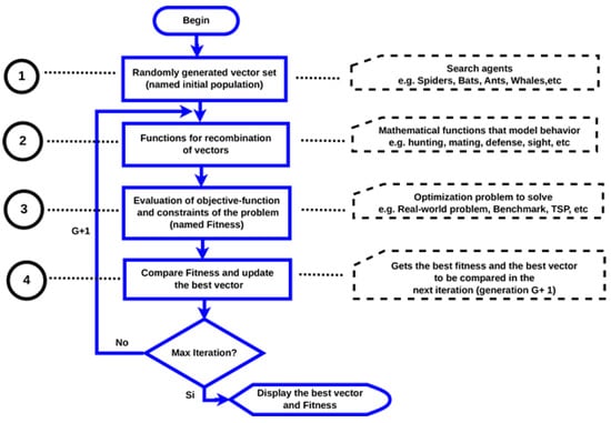
Figure 1.
General structure of a bio-inspired algorithm.
Phase 1: A set of vectors is randomly generated; the cardinality of the set is called the size of the initial population. The length of the vector is the number of variables in the problem (dimension). The vector represents the search agent, e.g., they can be used to represent some animals (reptiles, mammals, birds, amphibians, or insects), even some physical or chemical phenomenon. This initial population will evolve on each iteration.
Phase 2: Vector recombination functions (search agents). In this phase, the mathematical model that represents the behavior of the modeled living being is proposed, e.g., hunting, breeding, mating. Furthermore, the model must have a good balance (good ratio between) between exploration (diversification) and exploitation (intensification) of the search solution space (over the search solution space).
Phase 3: In this phase, the set of vectors are evaluated in the objective function, with or without restrictions, where the result of the evaluation of each vector is called fitness, for instance, the lowest fitness value is the best vector when the objective is to minimize.
Phase 4: The best fitness of the previous iteration (generation) is compared with the best fitness of the current iteration. If an obtained value exceeds (minimize) the best fitness obtained so far, the value and its respective vector are updated. In this way, in each iteration in the worst case, the fitness will be equal to that of the previous iteration, but it will never get worse. It is essential to highlight that the performance of a bio-inspired algorithm can be affected by the size of the population and the number of iterations.
Here, a new population-based bio-inspired algorithm, namely Jumping Spider Optimization Algorithm (JSOA), is proposed for solving optimization problems. JSOA mathematically models the persecution, search and jumping on the prey hunting strategies of jumping spiders. The rest of the paper is arranged as follows:
Section 2 illustrates the JSOA details, including the inspiration, mathematical model, time complexity, and a population size analysis. The proficiency and robustness of the proposed approach are benchmarked with several numerical examples, and their comparison with state-of-the-art metaheuristics are presented in Section 3. The results and discussion of the proposed algorithm are shown in Section 4. Real-world applications are solved in Section 5. The final section of the paper summarizes the conclusions and future work.
2. Jumping Spider Optimization Algorithm (JSOA)
In this section, the inspiration of the proposed method is first discussed. Then, the mathematical model is provided.
2.1. Biological Fundamentals
Jumping spiders Salticidae are found in a wide range of microhabitats [45]. Family Salticidae is the largest family of spiders; they are agile and dexterous jumpers of a few millimeters in length. They move at high speed and are capable of long and accurate jumps. They are generally active diurnal hunters and do not build webs. Their body appears to be covered with hairs that are both scaly, sometimes iridescent. The palps of males, but not females, are often large and showy, used during courtship. The front legs are somewhat larger and used to hold the prey when they fall on it. Thus, running and jumping on the prey are their primary hunting method. When they move from one side to the other and especially before jumping, they glue a silk thread where they are perched to protect themselves in case the jump fails. In that case, they climb back up the thread. The silk threads are impregnated with pheromones that play a role in reproductive and social—communication and possibly navigation. In addition, jumping spiders have complex eyes and acute vision. They are known for their bright colors and elaborate ornamentation, where males are generally brighter than females. Some species can remember and recognize colors and adapt their hunting style accordingly. Further details about the Jumping Spiders’ biology and locomotion behavior can be found in [46,47]. A photograph of the jumping spider can be seen in Figure 2.
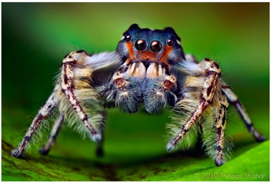
Figure 2.
Salticidae Jumping Spider. Photography by Thomas Shahan (published under a CC BY 2.0 license).
2.2. Mathematical Model and Optimization Algorithm
In this section, the mathematical model of Jumping spider’s different hunting strategies is first provided. The JSOA algorithm is then proposed. The hunting strategies considered are attacking by persecution, search, and Jumping on the prey. In addition, a model is also considered to represent the pheromone rate of the spider.
2.2.1. Strategy 1: Persecution
When the spider is not within a distance where it can catch its prey by jumping, it will move closer by doing some stealthy movements until it is at an achievable distance where it can jump and catch the prey. The persecution strategy can be represented by the uniformly accelerated rectilinear motion, see Equation (1). Thereby, the spider moves along the coordinate axis and the velocity increases (or decreases) linearly with time with constant acceleration.
where shows the position of ith follower spider, t is the time, is the initial speed. The acceleration is given by , where .
Here, for the optimization, each iteration is considered as the time, where the difference between iterations is equal to 1 and the initial speed is set to zero, . Thereby, Equation (1) can be re-defined as follows:
where is the new position of a search agent (jumping spider) for the generation g + 1, is the current ith search agent in generation g, and is the rth search agent randomly selected, with , where r is a random integer number generated in the interval from 1 to the size of a maximum of search agents. A representation of this strategy can be seen in Figure 3.
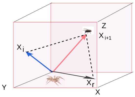
Figure 3.
Representation of Jumping Spider’s persecution strategy.
2.2.2. Strategy 2: Jumping on the Prey
The jumping spider follows its prey and pounces on it. The hunting strategy of jumping on the prey can be represented as a projectile motion; see Figure 4.
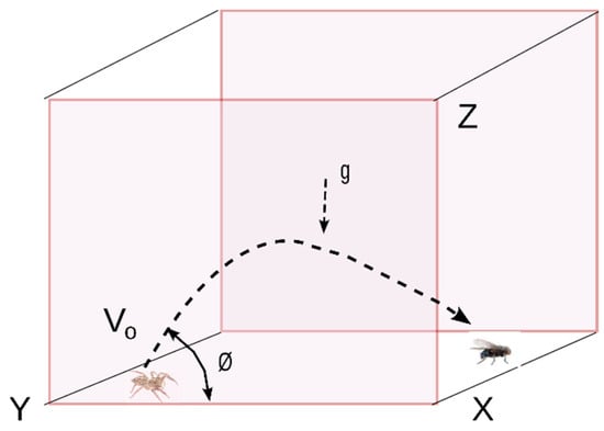
Figure 4.
Jumping on the prey [47].
The equations of projectile motion, which result from the composition of a uniform motion along the X-axis and a uniformly accelerated motion along the Y-axis, are as follows:
The horizontal axis and its derivative with respect to time is represented by Equation (3).
Similarly, the vertical axis, and its derivative with respect to time is represented by Equation (4).
The time is represented similarly to strategy 1. Thereby, we obtain the equation of the trajectory, as seen in Equation (5).
Finally, the trajectory depicted in Figure 4 can be expressed as follows:
where is the new position of a search agent, indicating jumping spiders’ movement), is the current ith search agent, is set to 100 mm/seg, g is the gravity (9.80665 ), and the angle is calculated by an angle value randomly generated between (0, 1).
2.2.3. Strategy 3: Searching for Prey
The Jumping spider performs a random search around the environment to locate prey. Two mathematical functions, local and global search, are proposed for the modeling of this search technique, see Figure 5.
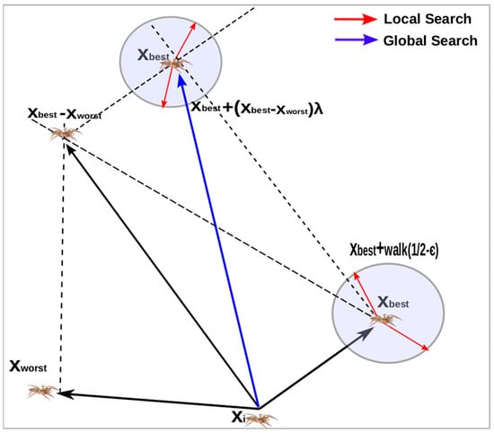
Figure 5.
Local and global search.
The local search is described in Equation (7)
where is the new position of a search agent, is the best search agent found from the previous iteration, walk is a pseudo-random number uniformly distributed in the interval of (−2, 2), whereas is a normally distributed pseudo-random number in the interval of (0, 1).
On the other hand, the Global search is formulated by Equation (8).
where, is the new position of a search agent, and are the best and worst search agent found form the previous iteration, respectively, and is a Cauchy random number with set to 0 and set to 1.
2.2.4. Strategy 4: Jumping Spider’ Pheromone Rates
The pheromones are chemical substances produced and secreted to the outside by an individual, they are olfactory perceived by other individuals of the same species, and they cause a behavior change. Pheromones are produced by many animals, among which are insects, including spiders. In some spiders, like black widow spiders, the pheromone has a notable role in the courtship-mating. Whereas, in the Jumping spider the courtship-mating is based on its striking colors. Nevertheless, they also produce pheromones; the modeling of the rate of pheromones is taken from [15] and defined in the following equation:
where and are the worst and the best fitness value in the current generation, respectively, whereas is the current fitness value of the ith search agent. Equation (9) normalize the fitness value in the interval (0, 1) where 0 is the worst pheromone rate, whereas 1 is the best.
The criteria consist that for low pheromones rates values equal or less than 0.3, the following equation is then applied [15]:
where is the search agent (jumping spider) with low pheromone rate that will be updated, and are random integer numbers generated in the interval from 1 to the maximum size of search agents, with , whereas and are the , th search agents selected, is the best search agent found from the previous iteration and is a binary number generated, . The pheromone procedure is shown in Algorithm 1.
| Algorithm 1 Pheromone procedure |
|
2.2.5. Pseudo Code for JSOA
The pseudocode for the JSOA is explained in Algorithm 2, whereas the overall flow is shown in Figure 6.
| Algorithm 2 Jumping Spider Optimizer Algorithm |
|
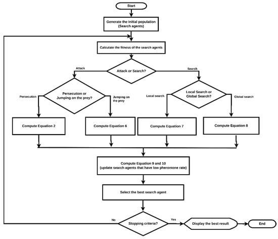
Figure 6.
JSOA flowchart.
2.3. JSOA Algorithm Analysis
In this section, an in-depth analysis of the JSOA algorithm is carried out. This analysis includes the JSOA’s time complexity and the associated effects of the population size in the algorithm’s performance.
2.3.1. Time Complexity
Without any loss of generality, let f be any optimization problem and suppose that O(f) is the computational time complexity of evaluating its function value. Thereby, the JSOA computational time complexity is defined as O (f * tMax * nSpiders), where tMax is the maximum number of iterations, and nSpiders is the number of spiders (population size).
2.3.2. Population Size Analysis
The effects of the population size on the performance of the JSOA algorithm are studied by fixing the number of iterations to 100 and then varying the population size initially at 50, then 100, 200, and 500 for the Griewank function (F2). The output of these tests is summarized in Figure 7, where a convergence graph is used to determine whether the measured quantity (fitness) converged acceptably. The results were graphically compared with the setup mentioned above. Whereas Figure 8 shows the JSOA algorithm compared with the four most recent bio-inspired algorithms from the first half-year of 2021, these are Coot Bird Algorithm (COOT) [16], Chaos Game Optimization (CGO) [42], Mexican Axolotl Optimization (MAO) [17], and Golden Eagle Optimizer (GEO) [18].
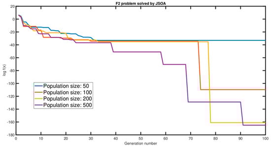
Figure 7.
Convergence graph of population size analysis.
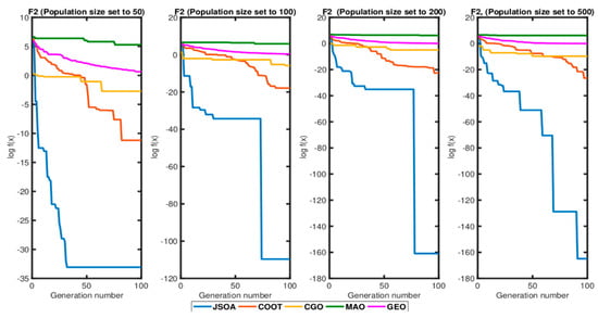
Figure 8.
JSOA, COOT, CGO, MAO, and GEO Convergence graph population size analysis.
Additionally, the algorithms were tested as micro-algorithms with a reduced number of iterations and population size of 30 and 50 respectively. Figure 9 shows the results of this analysis.
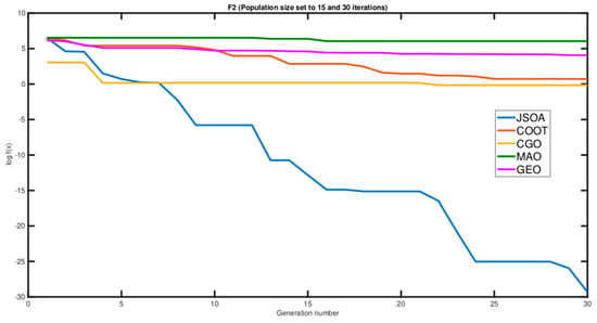
Figure 9.
Convergence graph of the population size analysis as micro-algorithms.
Notice that JSOA outperforms all the other algorithms, even as a micro-algorithm. Based on this, for the rest of the paper, JSOA tests will be conducted with a population size of 200 for testbench functions and 100 for real-world problems.
3. Experimental Setup
The numerical efficiency, effectiveness, and stability of the JSOA algorithm developed in this study were tested by solving 20 classical well-known benchmark optimization functions reported in the literature [48]. The classification of the testbench functions can be observed in Table A1. The unimodal functions allow testing the exploitation ability (local search) since they only have one global optimum [14]. In contrast, multimodal functions can test the exploration ability (global search) since they include many local optima [14]. Table A2 summarizes these testbench functions where Dim indicates the dimension of the function, Interval is the boundary of the function’s search space and is the optimum value. The shapes of the testbench functions considered in this study are shown in appendix A. The JSOA algorithm was compared with ten state-of-the-art bio-inspired algorithms taken from the literature; these are Coot Bird Algorithm (COOT) [16], Chaos Game Optimization (CGO) [42], Mexican Axolotl Optimization (MAO) [17], Golden Eagle Optimizer (GEO) [18], Archimedes Optimization algorithm (AOA) [21], Arithmetic Optimization Algorithm (ArOA) [22], Gradient-based Optimizer (GBO) [23], Hunger Game Search (HGS) [24], Henry Gas Solubility Optimization (HGSO) [25] and, Harris Hawks Optimization (HHO) [26]. For each testbench function, the eleven algorithms were run 30 times, the size of the population (search agents) and the number of iterations were set to 30 and 200, respectively. The entire parameter settings for all algorithms are shown in Table 1.

Table 1.
Parameter settings.
Our approach is implemented in MATLAB R2018a. All computations were carried out on a standard PC (Linux Kubuntu 20.04 LTS, Intel core i7, 2.50 GHz, 32 GB).
4. Results and Discussion
The comparison results are shown in Table 2, where , the best, the mean and standard deviation values are shown. The convergence graphs of all functions versus all algorithms selected in this study are summarized in Figure 10. In order to investigate the significant differences between the results of the proposed JSOA and the other algorithms, the Wilcoxon rank-sum non-parametric statistical test with a 5% degree of significance was carried out. This statistical test returns a parameter called p-values that determines the significance level of two algorithms. In this experimentation, an algorithm is statistically significant if and only if the calculated p-value is less than 0.05. Table 3 summarizes the result of this test.
Table 2.
JSOA—Performance and comparison.
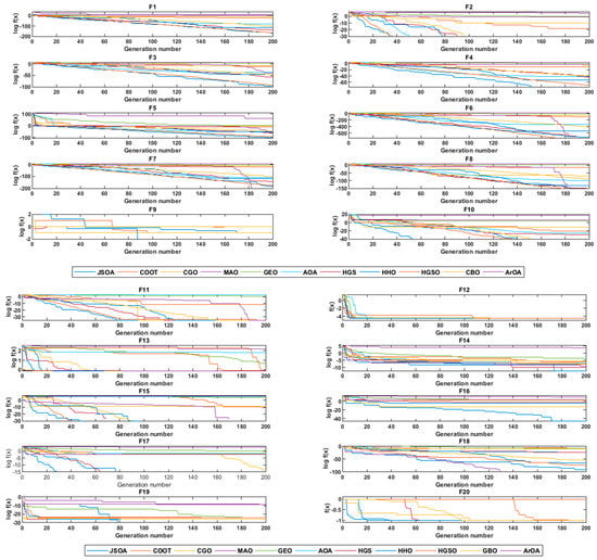
Figure 10.
Convergence curves.
Table 3.
The p-values of the Wilcoxon rank-sum test with 5% significance for JSOA vs. other algorithms (20 benchmark functions with 30 dimensions). NaN means “Not a Number” returned by the test.
Moreover, to evaluate the quality of the results the Mean Absolute Error (MAE) criteria was used to measure the error between the best-known (fitness) versus the mean fitness computed as described in Equation (11). See Table A2.
where indicates the mean of the optimal values (computed), is the corresponding global optimal value (observed), and n represents the number of test functions. Note that the arithmetic average of the absolute error is . It shows how far the results are from actual values. The ten algorithms were ranked by computing their Mean Absolute Error (MAE). Table 4 shows the average error rates obtained in the 20 testbench functions, while the ranking of all the algorithms based on their MAE calculations is illustrated in Table 5.
Table 4.
Error rates results (20 benchmark functions).
Table 5.
Rank of algorithms using MAE.
According to the statistical results given in Table 2, the Jumping Spider Optimization Algorithm (JSOA) can provide overtopping results. In the exploitation analysis (unimodal functions), the JSOA outperforms all algorithms in the functions F1, F3, F4, F5, and F10. Whereas competitive results were found in the functions F2, F6, F7, F8 and F9 for the Algorithms Chaos Game Optimization (CGO), Archimedes Optimization algorithm (AOA), Gradient-base Optimizer (GBO), Hunger Game Search (HGS), Henry Gas Solubility Optimization (HGSO), Harris Hawks Optimization (HHO), and Arithmetic Optimization Algorithm (ArOA). Moreover, in the exploration analysis, multimodal functions, the JSOA outperforms all algorithms in functions F14, F16, F17, F18, and F19. Whereas it also shows competitive results with the COOT, CBO, HGSO, HHO, HGS, and ArOA, for F11, F12, F3, F15 and F20 functions. On the other hand, in Wilcoxon rank-sum test the p-values in Table 3 confirm the meaningful advantage of JSOA compared to other bio-inspired algorithms for many cases. Additionally, in the Mean Absolute Error (MAE) analysis, the JSOA algorithm appears ranked in the second position with a slight difference of 1.43 × 10⁻² with the first position, as shown in Table 5.
In all the carried out tests, the number of iterations was set at 200, this being a lower value than that commonly used in the literature (500 or 1000) [16,17,18]. Therefore, the JSOA algorithm is more efficient in finding optimal (near-to optimal) solutions with a smaller number of iterations.
5. Real-World Applications
In this section, constrained optimization problems are considered. The JSOA algorithm was tested with four Real-World Single Objective Bound Constrained Numerical Optimization problems, Process Flow Sheeting, Process Synthesis, Optimal Design of an Industrial Refrigeration System and Welded Beam Design, taken from the CEC2020 special session [49].
On the other hand, the JSOA algorithm was also tested to find the optimal tuning parameters of a Proportional-Integral-Derivative (PID) controller and to solve the Selective Harmonics Elimination Problem, taken from [14,15], respectively.
For all the real-world application problems solved, JSOA was tested against COOT, CGO, MAO, GEO, and the best ranked in the MAE test (HHO), with population size and maximum iteration equal to 30 and 100, respectively.
5.1. Constraint Handling
The constraint handling method used is based on Penalization of Constraints (PCSt) [14] and in computing the Mean Constraint Violation (MCV) [49].
The PCSt handling is based on the penalization of infeasible solutions, that is at least one constraint is violated. This method is formulated in Equation (12) as follows:
where is the fitness function value of the worst feasible solution in the population, whereas is the fitness function value of a feasible solution and is the value of MCV. The MCV handling is depicted in Equation (13).
where is the sum of the p inequality constraints, whereas is the sum of the m equality constraints. and are formulated in Equations (14) and (15), respectively.
In the inequality constraint or the equality constraint is not violated, a zero value is returned, else its self-value is returned (the value of the constraint is violated). That is to say, the constraint handling method used is based on the fitness of an infeasible solution punished by the worst feasible solution in the current population plus the mean value of the constraints violated. In Equation (15), the value is set to 0.0001.
5.2. Process Flow Sheeting Problem
This problem is formulated as a non-convex constrained optimization problem [49]. In this test, there are three decision variables with three inequality constraints. It is formulated as shown in Equation (16). The best known feasible objective function value is
In Table 6, the comparison results show that JSOA, CGO, COOT, and HHO algorithms reported feasible solutions, whereas MAO and GEO are infeasible, as seen in the convergence graph in Figure 11. An infeasible solution does not satisfy one or more constraints, so it is not valid for the problem. The JSOA algorithm is ranked as the first best-obtained solution. The difference with the best-known feasible objective function value is 1.17347 × 10⁻⁵.
Table 6.
Process Flow Sheeting problem—Comparison Results.
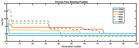
Figure 11.
Convergence graph of the Process Flow Sheeting Problem. The dotted line represents an infeasible solution shown by an algorithm.
5.3. Process Synthesis Problem
This problem has non-linearities in real and binary variables [50]. Here, there are seven decision variables and nine inequality constraints. The mathematical formulation of the optimization problem is described in Equation (17). The best known feasible objective function value is .
In Table 7, the comparison results show that JSOA and COOT algorithms reported feasible solutions, whereas MAO, CGO, GEO, and HHO are infeasible, as seen in the convergence graph in Figure 12. Note that the JSOA algorithm is ranked as the first best-obtained solution. The difference with the best-known feasible objective function value is 1.21 × 10⁴.
Table 7.
Comparison results for the Process Synthesis problem.
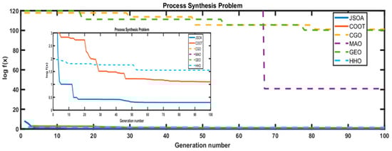
Figure 12.
Convergence graph of the Process Synthesis Problem. The dotted line represents an infeasible solution shown by an algorithm.
5.4. Optimal Design of an Industrial Refrigeration System
The problem is formulated as a non-linear inequality-constrained optimization problem [50]. Here, there are fourteen decision variables and 15th inequality constraints. The best-known feasible objective is . This problem can be stated as follows:
In Table 8, the comparison results show that JSOA and COOT algorithms reported feasible solutions, whereas MAO, CGO, GEO, and HHO are infeasible, as seen in the convergence graph illustrated in Figure 13. Note that the JSOA algorithm is ranked as the first best-obtained solution. The difference with the best-known feasible objective function value is 2.77 × 10⁻³.
Table 8.
Comparison results for the Optimal Design of an Industrial Refrigeration System.
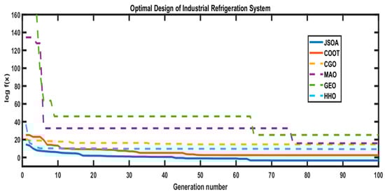
Figure 13.
Convergence graph of the Optimal Design of an Industrial Refrigeration System. The dotted line represents an infeasible solution shown by an algorithm.
5.5. Welded Beam Design
The main objective of this problem is to design a welded beam with minimum cost [50]. This problem contains five inequality constraints and four decision variables that are used to develop a welded beam [51]. The best known feasible objective function value is . Therefore, the mathematical description of this problem can be defined as follows:
In Table 9, the comparison results show that JSOA, MAO, COOT and GEO algorithms reported feasible solutions, whereas GEO and HHO are infeasible, as seen in the convergence graph in Figure 14. Furthermore, the COOT algorithm showed a competitive result, whereas the JSOA algorithm is ranked as the first best-obtained solution. The difference with the best-known feasible objective function value is 2.27 × 10⁻⁸.
Table 9.
Comparison results for Welded Beam Design.
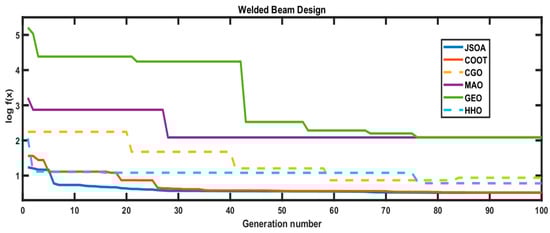
Figure 14.
Convergence graph of Welded Beam Design. The dotted line represents an infeasible solution shown by an algorithm.
5.6. Tuning of a Proportional-Integral-Derivative (PID) Controller: Sloshing Dynamics
Problem
This problem is taken from [14]. The goal is to tune a Proportional-Integral-Derivative (PID) controller for the Sloshing dynamics phenomenon (SDP). The SDP is a well-known problem in fluid dynamics. It is related to the movement of a liquid inside another object, altering the system dynamics [14]. Sloshing is an important effect on mobile vehicles carrying liquids, e.g., ships, spacecraft, aircraft, and trucks. A deficient sloshing control causes instability and accidents.
Sloshing dynamics can be depicted as a Ball and Hoop System (BHS). This effect illustrates the dynamics of a steel ball that is free to roll on the inner surface of a rotating circular hoop [52]. The ball exhibits an oscillatory motion caused by the continuously rotated hoop through a motor. The ball will tend to move in the direction of the hoop rotation and will fall back, at some point, when gravity overcomes the frictional forces [14]. Seven variables can describe the BHS behavior: hoop radius (R), hoop angle (), input torque to the hoop (T(t)), ball position on the hoop (y), ball radius (r), ball mass (m) and ball angles with vertical (slosh angle) () [14]. A schematic representation is shown in Figure 15. The transfer function of the BHS system, taken from [14], is formulated in Equation (20). Where θ is, the input and y are the output of the BHS system.
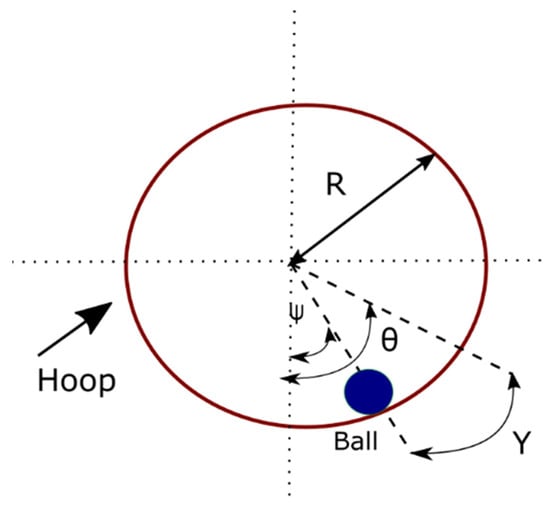
Figure 15.
Schema of the ball and hoop system [14].
Table 10 summarizes the comparison results at solving the BHS for the optimal tuning of a Proportional-Integral Derivative (PID) controller. The transient response parameters of the PID controller are Rise time, Settling time, Peak time, and Peak overshoot. The PID controller is designed to minimize the overshoot and settling time so that the liquid can remain as stable as possible under any perturbance, and if it moves, it can rapidly go back to its steady-state [14]. It is to be noticed that the JSOA and HHO show competitive results and are better than the rest of the algorithms part of this test, obtaining the lowest rising and settling time value, as well as the peak overshoot, see Table 11. In addition, the PID controller step response for the six algorithms is shown in Figure 16. This figure shows that the JSOA (blue line) and HHO (magenta line) are more stable with very fine control without exceeding the setpoint (dotted line).
Table 10.
Comparison results of optimized PID parameters.
Table 11.
Comparison results of transient response parameters.
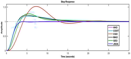
Figure 16.
Comparative results of step response for the PID controller.
5.7. Selective Harmonics Elimination (SHE) Problem
The selective harmonic elimination (SHE) problem is taken from [15]; it is a highly used control strategy applied to multilevel inverters (MLI) that aims for the elimination of unwanted low order harmonics by setting them equal to zero. In contrast, the fundamental component is kept equal to the desired amplitude. Figure 17 shows the typical staircase output waveform of a single-phase multilevel inverter. This waveform is generated by the correct synchronization and angle switching of the MLI power semiconductor devices, part of cascaded H-bridge inverter modules with isolated direct current (dc) sources, connected either in cascaded or series.
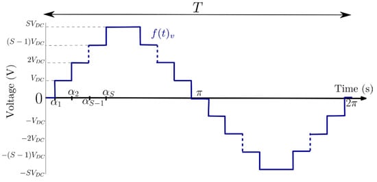
Figure 17.
Single phase multilevel inverter staircase output waveform [15].
The Fourier series expansion of this waveform is defined in Equation (21). Due to the quarter-wave symmetry nature of the waveform, the dc component, and the Fourier coefficient will be both equal to 0.
By Fourier transforming the staircase output waveform, it can be described in Equation (22).
Therefore, a series of nonlinear equations must be solved for unknown angles. The mathematical relationship between the MLI isolated dc sources (S) and the number of levels (n) is shown in Equation (23).
where the switching angles () are subjected to:
As a case of study, a eleven-levels multilevel inverter is selected with an index of modulation equal to 1. Thus, the selective harmonic elimination set of equations that eliminates the fifth, seventh, eleventh and thirteenth harmonic can be rewritten as below:
where and the modulation index is defined as for . is defined as the desired peak voltage and is equal to the direct voltage of the isolated dc power supplies.
Therefore, the objective function [15], is defined as:
Subjected to the switching angles described in Equation (24). Some of the algorithms that are chosen for comparison are Whale Optimization Algorithm (WOA), Modified Grey Wolf Optimization Algorithm (MGWOA) and Black Widow Optimization Algorithm (BWOA). Table 5 was taken from [15] and updated with results of the following algorithms: Coot Bird Algorithm (COOT) [16], Chaos Game Optimization (CGO) [42], Mexican Axolotl Optimization (MAO) [17], Golden Eagle Optimizer (GEO) [18], Harris Hawks Optimization (HHO)[26], and Jumping Spider Optimization Algorithm (JSOA). The obtained near-optimal angles are then fed to a Simulink code that retrieves the staircase output waveform. Then, the Total Harmonic Distortion (THD) is calculated, and a Fourier spectrum is determined to show the correct elimination of the unwanted low order harmonics. From Table 12, it can be seen that JSOA gets the best fitness values, whereas Figure 18 shows the correct elimination of the fifth, seventh, eleventh, and thirteenth order harmonics.
Table 12.
Comparison results for the selective harmonic elimination problem.
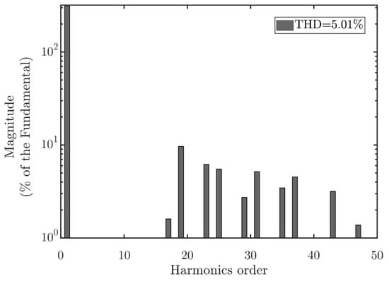
Figure 18.
Fourier transform spectrum calculated from the JSOA set of angles described in Table 12.
6. Conclusions
This work presented a new swarm-based optimization algorithm inspired by the hunting behavior Arachnida Salticidae, named Jumping Spider Optimization Algorithm (JSOA). The proposed method included three operators to simulate the spider hunting methods (search, persecution, and jumping on the prey). These strategies work as mathematical recombination functions of vectors (spiders, also named search agents), that provide a fine balance between exploitation and exploration over the solution search space. The algorithm’s performance was benchmarked on 20 test functions, four real-world optimization problems, tuning of a Proportional-Integral-Derivative (PID) controller, and the selective harmonic elimination problem. In addition, the performance of the proposed JSOA algorithm is compared with the ten most recent algorithms in the literature: COOT, CGO, MAO, GEO, AOA, ArOA, GBO, HGS, HGSO, and HHO. The statistical results show that the JSOA algorithm outperforms or has competitive results in these algorithms. This study has the following conclusions:
- The JSOA algorithm does not have parameters to configure affecting its performance.
- Exploitation and exploration of the JSOA are intrinsically high on problems involving unimodal and multimodal test functions, respectively.
- The algorithm has outstanding results with few iterations, 200 for the testbench functions and 100 for the real-world problems.
- The JSOA algorithm models the pheromone of spiders whose criteria are used to repair vectors with a low pheromone level. The vectors (spiders, also named search agents) with the worst fitness are replaced in each iteration. This repair helps get a better performance in the exploration of the search space.
- The Wilcoxon rank-sum test p-values confirm the meaningful advantage of JSOA compared to other bio-inspired algorithms for many cases. In addition, the MAE statistical results show that the JSOA is ranked among the highest position compared to the other algorithms.
- JSOA can tune a Proportional-Integral-Derivative (PID) controller with very fine control without exceeding the setpoint, with zero percent of peak overshoot for the Sloshing dynamics Problem.
- JSOA can solve the Selective Harmonic Elimination problem with the best fitness value results compared to WOA, MGWOA, BWOA, COOT, CGO, MAO, GEO, and HHO algorithms and competitive results with the BWOA algorithm regarding the Total Harmonic Distortion (THD)
- JSOA can solve real-world problems with unknown search spaces.
The evaluation criterion of the pheromone rate lacks a sensitivity analysis of the fixed 0.3 value previously determined empirically. An updated version of the JSOA algorithm addressing this issue and that solves multi and many-objective functions is currently under development for future work
Author Contributions
Conceptualization, H.P.-V.; methodology, H.P.-V.; software, H.P.-V. and A.P.-D.; validation, P.R., C.B. and A.B.M.-C.; formal analysis, A.C. and A.P.-D.; investigation, P.R., C.B. and A.B.M.-C.; resources, H.P.-V.; data curation, A.P.-D. and A.C.; writing—original draft preparation, H.P.-V.; writing—review and editing, H.P.-V., A.P.-D. and P.R.; visualization, C.B. and A.B.M.-C.; supervision, H.P.-V. and A.P.-D.; project administration, H.P.-V.; funding acquisition, H.P.-V. All authors have read and agreed to the published version of the manuscript.
Funding
This research was funded by Instituto Politécnico Nacional (IPN) through grant number SIP-20211364.
Institutional Review Board Statement
Not applicable.
Informed Consent Statement
Not applicable.
Data Availability Statement
The source code used to support the findings of this study has been deposited in the MathWorks repository at https://www.mathworks.com/matlabcentral/fileexchange/104045-a-bio-inspired-method-inspired-by-arachnida-salticidade (accessed on 16 October 2021).
Conflicts of Interest
The authors declare no conflict of interest.
Appendix A
Table A1.
Classification of Testbench functions.
Table A1.
Classification of Testbench functions.
| ID | Function Name | Unimodal | Multimodal | n-Dimensional | Non-Separable | Convex | Differentiable | Continuous | Non-Convex | Non-Differentiable | Separable | Random |
|---|---|---|---|---|---|---|---|---|---|---|---|---|
| F1 | Brown | X | X | X | X | X | ||||||
| F2 | Griewank | X | X | X | X | X | ||||||
| F3 | Schwefel 2.20 | X | X | X | X | X | X | |||||
| F4 | Schwefel 2.21 | X | X | X | X | X | X | |||||
| F5 | Schwefel 2.22 | X | X | X | X | X | X | |||||
| F6 | Schwefel 2.23 | X | X | X | X | X | X | |||||
| F7 | Sphere | X | X | X | X | X | X | |||||
| F8 | Sum Squares | X | X | X | X | X | X | |||||
| F9 | Xin-She Yang N. 3 | X | X | X | X | X | ||||||
| F10 | Zakharov | X | X | X | X | |||||||
| F11 | Ackley | X | X | X | X | X | ||||||
| F12 | Ackley N. 4 | X | X | X | X | X | ||||||
| F13 | Periodic | X | X | X | X | X | X | |||||
| F14 | Quartic | X | X | X | X | X | X | |||||
| F15 | Rastrigin | X | X | X | X | X | X | |||||
| F16 | Rosenbrock | X | X | X | X | X | X | |||||
| F17 | Salomon | X | X | X | X | X | X | |||||
| F18 | Xin-She Yang | X | X | X | X | X | ||||||
| F19 | Xin-She Yang N. 2 | X | X | X | X | X | ||||||
| F20 | Xin-She Yang N. 4 | X | X | X | X | X |
Table A2.
Description of the Testbench Functions.
Table A2.
Description of the Testbench Functions.
| ID | Function | Dim | Interval | |
|---|---|---|---|---|
| F1 | 30 | [−1, 4] | 0 | |
| F2 | 30 | [−600, 600] | 0 | |
| F3 | 30 | [−100, 100] | 0 | |
| F4 | 30 | [−100, 100] | 0 | |
| F5 | 30 | [−100, 100] | 0 | |
| F6 | 30 | [−10, 10] | 0 | |
| F7 | 30 | [−5.12, 5.12] | 0 | |
| F8 | 30 | [−10, 10] | 0 | |
| F9 | 30 | [−2π, 2π], m = 5, β = 15 | −1 | |
| F10 | 30 | [−5, 10] | 0 | |
| F11 | 30 | [−32, 32], a = 20, b = 0.3, c = 2π | 0 | |
| F12 | 2 | [−35, 35] | −5.901 × 10¹⁴ | |
| F13 | 30 | [−10, 10] | 0.9 | |
| F14 | 30 | [−1.28, 1.28] | 0 + random noise | |
| F15 | 30 | [−5.12, 5.12] | 0 | |
| F16 | 30 | [−5, 10] | 0 | |
| F17 | 30 | [−100, 100] | 0 | |
| F18 | 30 | [−5, 5], random | 0 | |
| F19 | 30 | [−2π, 2π] | 0 | |
| F20 | 30 | [−10, 10] | −1 |
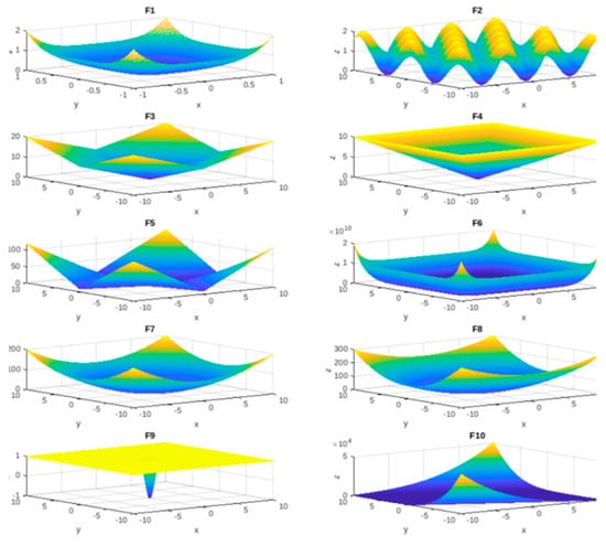
Figure A1.
Testbench Unimodal functions.
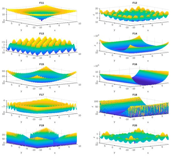
Figure A2.
Testbench Multimodal functions.
References
- Kumar, A. Application of nature-inspired computing paradigms in optimal design of structural engineering problems—A review. Nat.-Inspired Comput. Paradig. Syst. 2021, 63–74. [Google Scholar] [CrossRef]
- Shaukat, N.; Ahmad, A.; Mohsin, B.; Khan, R.; Khan, S.U.-D.; Khan, S.U.-D. Multiobjective Core Reloading Pattern Optimization of PARR-1 Using Modified Genetic Algorithm Coupled with Monte Carlo Methods. Sci. Technol. Nucl. Install. 2021, 2021, 1–13. [Google Scholar] [CrossRef]
- Lodewijks, G.; Cao, Y.; Zhao, N.; Zhang, H. Reducing CO₂ Emissions of an Airport Baggage Handling Transport System Using a Particle Swarm Optimization Algorithm. IEEE Access 2021, 9, 121894–121905. [Google Scholar] [CrossRef]
- Malik, H.; Iqbal, A.; Joshi, P.; Agrawal, S.; Bakhsh, F.I. (Eds.) Metaheuristic and Evolutionary Computation: Algorithms and Applications; Springer: Berlin/Heidelberg, Germany, 2021; Volume 916. [Google Scholar] [CrossRef]
- Elaziz, M.A.; Dahou, A.; Abualigah, L.; Yu, L.; Alshinwan, M.; Khasawneh, A.M.; Lu, S. Advanced metaheuristic optimization techniques in applications of deep neural networks: A review. Neural Comput. Appl. 2021, 33, 14079–14099. [Google Scholar] [CrossRef]
- Wolpert, D.H.; Macready, W.G. No free lunch theorems for optimization. IEEE Trans. Evol. Comput. 1997, 1, 67–82. [Google Scholar] [CrossRef] [Green Version]
- Ho, Y.; Pepyne, D. Simple Explanation of the No-Free-Lunch Theorem and Its Implications. J. Optim. Theory Appl. 2002, 115, 549–570. [Google Scholar] [CrossRef]
- Mirjalili, S.; Song Dong, J.; Lewis, A.; Sadiq, A.S. Particle Swarm Optimization: Theory, Literature Review, and Application in Airfoil Design. In Nature-Inspired Optimizers: Theories, Literature Reviews and Applications; Mirjalili, S., Song Dong, J., Lewis, A., Eds.; Springer International Publishing: Cham, Switzerland, 2020; pp. 167–184. [Google Scholar]
- Castelli, M.; Manzoni, L.; Mariot, L.; Nobile, M.S.; Tangherloni, A. Salp Swarm Optimization: A critical review. Expert Syst. Appl. 2021, 189, 116029. [Google Scholar] [CrossRef]
- Mirjalili, S.; Lewis, A. The Whale Optimization Algorithm. Adv. Eng. Softw. 2016, 95, 51–67. [Google Scholar] [CrossRef]
- Braik, M.S. Chameleon Swarm Algorithm: A bio-inspired optimizer for solving engineering design problems. Expert Syst. Appl. 2021, 174, 114685. [Google Scholar] [CrossRef]
- Jiang, Y.; Wu, Q.; Zhu, S.; Zhang, L. Orca predation algorithm: A novel bio-inspired algorithm for global optimization problems. Expert Syst. Appl. 2021, 188, 116026. [Google Scholar] [CrossRef]
- Abdollahzadeh, B.; Gharehchopogh, F.S.; Mirjalili, S. African vultures optimization algorithm: A new nature-inspired metaheuristic algorithm for global optimization problems. Comput. Ind. Eng. 2021, 158, 107408. [Google Scholar] [CrossRef]
- Peraza-Vázquez, H.; Peña-Delgado, A.F.; Echavarría-Castillo, G.; Morales-Cepeda, A.B.; Velasco-Álvarez, J.; Ruiz-Perez, F. A Bio-Inspired Method for Engineering Design Optimization Inspired by Dingoes Hunting Strategies. Math. Probl. Eng. 2021, 2021, 1–19. [Google Scholar] [CrossRef]
- Peña-Delgado, A.F.; Peraza-Vázquez, H.; Almazán-Covarrubias, J.H.; Cruz, N.T.; García-Vite, P.M.; Morales-Cepeda, A.B.; Ramirez-Arredondo, J.M. A novel bio-inspired algorithm applied to selective harmonic elimination in a three-phase eleven-level inverter. Math. Probl. Eng. 2020, 2020, 1–10. [Google Scholar] [CrossRef]
- Naruei, I.; Keynia, F. A new optimization method based on COOT bird natural life model. Expert Syst. Appl. 2021, 183, 115352. [Google Scholar] [CrossRef]
- Villuendas-Rey, Y.; Velázquez-Rodríguez, J.; Alanis-Tamez, M.; Moreno-Ibarra, M.-A.; Yáñez-Márquez, C. Mexican Axolotl Optimization: A Novel Bioinspired Heuristic. Mathematics 2021, 9, 781. [Google Scholar] [CrossRef]
- Mohammadi-Balani, A.; Nayeri, M.D.; Azar, A.; Taghizadeh-Yazdi, M. Golden eagle optimizer: A nature-inspired metaheuristic algorithm. Comput. Ind. Eng. 2021, 152, 107050. [Google Scholar] [CrossRef]
- Abualigah, L.; Shehab, M.; Alshinwan, M.; Mirjalili, S.; Elaziz, M.A. Ant Lion Optimizer: A Comprehensive Survey of Its Variants and Applications. Arch. Comput. Methods Eng. 2021, 28, 1397–1416. [Google Scholar] [CrossRef]
- Salehan, A.; Deldari, A. Corona virus optimization (CVO): A novel optimization algorithm inspired from the Corona virus pandemic. J. Supercomput. 2021. [Google Scholar] [CrossRef]
- Hashim, F.A.; Hussain, K.; Houssein, E.H.; Mabrouk, M.S.; Al-Atabany, W. Archimedes optimization algorithm: A new metaheuristic algorithm for solving optimization problems. Appl. Intell. 2021, 51, 1531–1551. [Google Scholar] [CrossRef]
- Abualigah, L.; Diabat, A.; Mirjalili, S.; Elaziz, M.A.; Gandomi, A.H. The Arithmetic Optimization Algorithm. Comput. Methods Appl. Mech. Eng. 2021, 376, 113609. [Google Scholar] [CrossRef]
- Ahmadianfar, I.; Bozorg-Haddad, O.; Chu, X. Gradient-based optimizer: A new metaheuristic optimization algorithm. Inf. Sci. 2020, 540, 131–159. [Google Scholar] [CrossRef]
- Yang, Y.; Chen, H.; Heidari, A.A.; Gandomi, A.H. Hunger games search: Visions, conception, implementation, deep analysis, perspectives, and towards performance shifts. Expert Syst. Appl. 2021, 177, 114864. [Google Scholar] [CrossRef]
- Hashim, F.A.; Houssein, E.H.; Mabrouk, M.S.; Al-Atabany, W.; Mirjalili, S. Henry gas solubility optimization: A novel physics-based algorithm. Future Gener. Comput. Syst. 2019, 101, 646–667. [Google Scholar] [CrossRef]
- Heidari, A.A.; Mirjalili, S.; Faris, H.; Aljarah, I.; Mafarja, M.; Chen, H. Harris hawks optimization: Algorithm and applications. Future Gener. Comput. Syst. 2019, 97, 849–872. [Google Scholar] [CrossRef]
- Singh, S.; Tiwari, A.; Agrawal, S. Differential Evolution Algorithm for Multimodal Optimization: A Short Survey. In Advances in Intelligent Systems and Computing; Springer: Berlin/Heidelberg, Germany, 2021; pp. 745–756. [Google Scholar]
- Katoch, S.; Chauhan, S.S.; Kumar, V. A review on genetic algorithm: Past, present, and future. Multimed. Tools Appl. 2021, 80, 8091–8126. [Google Scholar] [CrossRef] [PubMed]
- Liu, W.-L.; Yang, J.; Zhong, J.; Wang, S. Genetic programming with separability detection for symbolic regression. Complex Intell. Syst. 2021, 7, 1185–1194. [Google Scholar] [CrossRef]
- Sang, X.; Liu, X.; Zhang, Z.; Wang, L. Improved Biogeography-Based Optimization Algorithm by Hierarchical Tissue-Like P System with Triggering Ablation Rules. Math. Probl. Eng. 2021, 2021, 1–24. [Google Scholar] [CrossRef]
- Fu, Y.; Zhou, M.; Guo, X.; Qi, L.; Sedraoui, K. Multiverse Optimization Algorithm for Stochastic Biobjective Disassembly Sequence Planning Subject to Operation Failures. In Proceedings of the Transactions on System, Man, and Cybernetics: Systems, Virtual. 17–20 October 2021. [Google Scholar] [CrossRef]
- Kaur, A.; Kumar, Y. A new metaheuristic algorithm based on water wave optimization for data clustering. Evol. Intell. 2021, 1–25. [Google Scholar] [CrossRef]
- Kaveh, A.; Dadras, A. A novel meta-heuristic optimization algorithm: Thermal exchange optimization. Adv. Eng. Softw. 2017, 110, 69–84. [Google Scholar] [CrossRef]
- Kaveh, A. Advances in Metaheuristic Algorithms for Optimal Design of Structures; Springer: Cham, Switzerland, 2021. [Google Scholar] [CrossRef]
- Geem, Z.W.; Kim, J.H.; Loganathan, G.V. A new heuristic optimization algorithm: Harmony search. Simulation 2001, 76, 60–68. [Google Scholar] [CrossRef]
- Abbasi, M.; Abbasi, E.; Mohammadi-Ivatloo, B. Single and multi-objective optimal power flow using a new differen-tial-based harmony search algorithm. J. Ambient. Intell. Humaniz. Comput. 2020, 12, 851–871. [Google Scholar] [CrossRef]
- Braik, M.; Ryalat, M.H.; Al-Zoubi, H. A novel meta-heuristic algorithm for solving numerical optimization problems: Ali Baba and the forty thieves. Neural Comput. Appl. 2021, 1–47. [Google Scholar] [CrossRef]
- Qi, Y.; Liu, J.; Yu, J. A Fireworks algorithm based path planning method for amphibious robot. In Proceedings of the 2021 IEEE International Conference on Real-time Computing and Robotics (RCAR), Xining, China, 15–19 July 2021. [Google Scholar] [CrossRef]
- Tan, Y.; Zhu, Y. Fireworks Algorithm for Optimization. In Lecture Notes in Computer Science; Springer Science and Business Media LLC: Berlin/Heidelberg, Germany, 2010; pp. 355–364. [Google Scholar]
- Osaba, E.; Yang, X.-S. Soccer-Inspired Metaheuristics: Systematic Review of Recent Research and Applications. Appl. Optim. Swarm Intell. 2021, 81–102. [Google Scholar] [CrossRef]
- Gabis, A.B.; Meraihi, Y.; Mirjalili, S.; Ramdane-Cherif, A. A comprehensive survey of sine cosine algorithm: Variants and applications. Artif. Intell. Rev. 2021, 54, 5469–5540. [Google Scholar] [CrossRef] [PubMed]
- Talatahari, S.; Azizi, M. Chaos Game Optimization: A Novel Metaheuristic Algorithm; Springer: Berlin/Heidelberg, Germany, 2021; Volume 54. [Google Scholar] [CrossRef]
- Sasmito, A.; Pratiwi, A.B. Stochastic fractal search algorithm in permutation flowshop scheduling problem. In Proceedings of the International Conference on Mathematics, Computational Sciences and Statistics 2020, Online. 29 September 2020; Volume 2329, p. 050003. [Google Scholar] [CrossRef]
- Karami, H.; Sanjari, M.J.; Gharehpetian, G.B. Hyper-Spherical Search (HSS) algorithm: A novel meta-heuristic algorithm to optimize nonlinear functions. Neural Comput. Appl. 2014, 25, 1455–1465. [Google Scholar] [CrossRef]
- Aguilar-Arguello, S.; Taylor, A.H.; Nelson, X.J. Jumping spiders attend to information from multiple modalities when preparing to jump. Anim. Behav. 2021, 171, 99–109. [Google Scholar] [CrossRef]
- Göttler, C. Locomotion of Spiders—What Robotics can Learn from Spiders and Vice Versa. Ph.D. Thesis, ETH Zurich, Zurich, Switzerland, 2021. [Google Scholar] [CrossRef]
- Brandt, E.E.; Sasiharan, Y.; Elias, D.O.; Mhatre, N. Jump takeoff in a small jumping spider. J. Comp. Physiol. A 2021, 207, 153–164. [Google Scholar] [CrossRef] [PubMed]
- GitHub-Mazhar-Ansari-Ardeh/BenchmarkFcns: A Collection of Mathematical Test Functions for Benchmarking Optimization Algorithms. Available online: https://github.com/mazhar-ansari-ardeh/BenchmarkFcns (accessed on 20 October 2021).
- Suganthan, P.N.; Hansen, N.; Liang, J.J.; Deb, K.; Chen, Y.P.; Auger, A.; Tiwari, S. Problem Definitions and Evaluation Criteria for the CEC 2005 Special Session on Real-Parameter Optimization; Nanyang Technological University: Singapore, 2005. [Google Scholar]
- Kumar, A.; Wu, G.; Ali, M.Z.; Mallipeddi, R.; Suganthan, P.N.; Das, S. A test-suite of non-convex constrained optimization problems from the real-world and some baseline results. Swarm Evol. Comput. 2020, 56, 100693. [Google Scholar] [CrossRef]
- Vazquez, H.P.; Torres-Huerta, A.M.; Flores-Vela, A. Self-Adaptive Differential Evolution Hyper-Heuristic with Applications in Process Design. Comput. Sist. 2016, 20, 173–193. [Google Scholar] [CrossRef]
- Jain, N.; Parmar, G.; Gupta, R.; Khanam, I. Performance evaluation of GWO/PID approach in control of ball hoop system with different objective functions and perturbation. Cogent Eng. 2018, 5, 1465328. [Google Scholar] [CrossRef]
Publisher’s Note: MDPI stays neutral with regard to jurisdictional claims in published maps and institutional affiliations. |
© 2021 by the authors. Licensee MDPI, Basel, Switzerland. This article is an open access article distributed under the terms and conditions of the Creative Commons Attribution (CC BY) license (https://creativecommons.org/licenses/by/4.0/).