The Influence of Global Financial Liquidity on the Indonesian Economy: Dynamic Analysis with Threshold VAR

Abstract

Empirical studies of the global liquidity spillover on Indonesia’s economy are still relatively limited. Most of the global contagion literature on Indonesia’s economy focuses only on the effects of real shock (on output) due to financial shock. We assert that the effect of global output on Indonesia macroeconomic conditions is a fairly relevant issue to be studied. This research aims to investigate the interdependent relationships between world GDP, world commodity prices, world inflation, trade flows, capital inflow, capital account transactions, reserve accumulation, global liquidity (e.g., global broad money), and monetary aggregates, with regard to Indonesia’s GDP variables and inflation. This paper uses threshold vector autoregression (TVAR) to capture regime changes in the variables of the world economy. World economic data and Indonesia’s economic data were utilized to prove different responses to the world economic situation in two different regimes. This research identified two groups of upper regime and lower regime world variables—namely, world inflation, world GDP, and world commodity prices. TVAR estimation resulted in a smaller residual sum of squares compared to VAR estimation. Different regimes resulted in differences in Indonesia’s economic responses due to the shock of world economic variables. The findings generated by this research are expected to be insightful to monetary policymakers in Indonesia.

1. Introduction

For more than two decades after the Cold War, the world economy was increasingly integrated, in terms of both trade—through various free trade agreements—and financial aspects. Aizenman et al. (2008) found that the level of financial openness in both developed and emerging countries in Asia and Latin America tended to increase over the period of 1991–2006, along with the lax rules of international exchange flows and international capital flows. The activities of multinational corporations and financial innovations—such as corporate bond issuance and stock listing abroad—also further complicate the inter-state financial linkages in the present (Azis and Shin 2013). These global monetary and financial conditions are generally summarized under the umbrella term “global liquidity”, which refers to the availability of funding in global financial markets. Even so, in popular discourse, the term global liquidity is often used for more specific matters, such as monetary policy in developed countries or inter-state capital flows, which are more accurately considered to be a subset of the global liquidity issues (Domanski et al. 2011).

Other aspects of the global economy that often become concerns are global production, global inflation, and global commodity prices. These three variables play a notable role in the economic development of developing countries. For developing countries, economic development is measured by several variables, including GDP, inflation, trade flow, capital inflow, capital account transactions, and foreign exchange, among others (Aizenman et al. 2008). As identified by Azis and Shin (2013), the first surge period (1995Q4–1998Q2) culminated in the Asian financial crisis, while the second surge (2006Q4–2008Q2) was closely related to the credit boom that created preconditions for the global financial crisis. The current global economy may be in a third surge, fueled by a highly accommodative monetary policy in the wake of global recession, along with high commodity prices.

The roles of several variables—such as GDP, inflation, trade flow, capital inflow, capital account transactions, and foreign exchange—affect the influence of global variables on GDP and inflation in developing countries. For most countries, foreign exchange accumulation is a logical response to a possible reversal of capital flows at all times, and to reduce the adverse impacts of economic openness on exchange rate movements (Aizenman et al. 2008). However, the accumulation of foreign exchange may erode global financial stability by having the bulk of financial instruments invested in developed countries, thereby improving only these countries’ financial conditions (Domanski et al. 2011; Landau 2013).

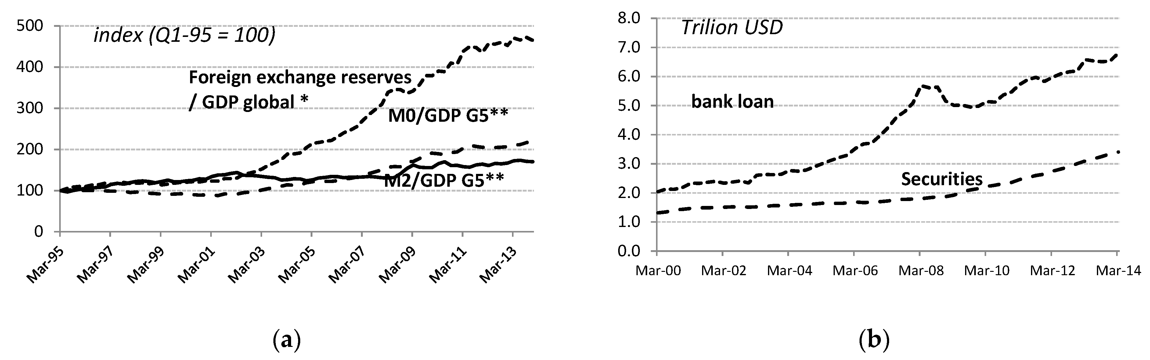
As one of the emerging Asian countries, Indonesia did not escape the phenomenon of this financial integration. Indonesia’s capital inflows have shown an upward trend relative to GDP and inflation since the end of the Asian crisis. The percentage of Indonesian financial assets held by foreigners has also shown an upward trend over the past eight years (Figure 1a; “*” indicates the total loan from the US, European Union, and Japan, while “**” represents finance from the US, European Union, Japan, UK, and Canada). The fluctuations now tend to be more extreme (Figure 1b). In line with this, the awareness of economic actors and takeover policies in Indonesia is increasing about the vulnerability of domestic economic conditions to fluctuations in global liquidity.

Empirical studies of the global liquidity spillover on Indonesia’s economy are still relatively limited. Most of the global contagion literature on Indonesia’s economy (Pratomo 2013) focuses only on the effects of real shock (on output) due to financial shock; in contrast, fluctuations in financial indicators often precede and predict changes in Indonesia’s GDP (Ng 2011). Several other studies have examined the impact of global liquidity on Indonesia in more specific contexts, such as the work of Yiu and Sahminan (2015), who studied the relationship between capital inflow and property prices. Based on these considerations, we believe that global output’s effect on Indonesia’s macroeconomic conditions is a reasonably relevant issue to be studied.

Matsumoto’s study (2011) provides a helpful framework for studying the impacts of worldwide production—particularly in Indonesia, where such research remains restricted. The main aim of this research is to identify the interdependent relationships between world GDP, world commodity prices, world inflation, with regard to Indonesia’s GDP variables and inflation. These relationships can consist of dynamic, direct, and indirect relationships. The appropriate analytical model for analyzing this relationship is vector autoregression (VAR). The VAR method used in this research allows us to detect the heterogeneity of Indonesia’s output, as well as inflation, in response to the shock of certain global variables. This statement is crucial, considering that several other studies (Sousa and Zaghini 2007) concluded that the impacts of global factors on economic circumstances in different nations might vary significantly. These variations can be linked to variations in each country’s financial systems. The standard VAR model was developed into a threshold VAR model because of the nonlinearity of response variables at various levels.

This paper describes different responses to certain situation variables, whereas other studies assume that the variables respond the same way in all situations. In reality, for different world GDP regimes, the economies of small countries will respond with different magnitudes. This study determines the appropriate threshold values for several global variables that separate the different regimes.

This study’s contribution to the literature is the provision of a research perspective wherein the response or impact of exogenous variables on endogenous variables may vary. This study suggests an idea of the existence of a threshold value as a limit for the occurrence of differences in responses to the global financial liquidity regime. Afonso et al. (2018) used a threshold VAR analysis to study the linkages between changes in the debt ratio, economic activity, and financial stress within different financial regimes. Chowdhury and Ham (2009) used TVAR because they assumed that low-to-moderate inflation is favorably related to economic growth in some developing countries. After a certain threshold, the level of inflation will undermine growth. Romyen et al. (2019) used the threshold gross domestic product (GDP) because, at high GDP, the impact of exports on GDP will be higher than at low GDP.

After this introduction, there will be a discussion of the theoretical background, followed by a review of the relevant literature. There then follows a description of the methodology, and the data and results are analyzed. Finally, there are several conclusions. The Indonesian economy will respond in different ways to the changing world economy. The disclosure of the threshold of world economic variables implies that the world economy being above the threshold will cause the Indonesian economy to be different if it is below its threshold value. A significant threshold value indicates that the nonlinear model is better than the linear model. The nonlinear model is better for identifying Indonesia’s economic response at the level of the world economy, which often fluctuates.

2. Theoretical Background

The main theory of this paper is based on the monetary modeling of Christiano and Eichenbaum (1992). Greater liquidity lowers the nominal interest rate in the short term (liquidity impact) and, hence, decreases loan costs and boosts asset prices as the discount rate decreases. Additionally, if prices and wages suffer temporary nominal rigidity, liquidity expansion will also increase inflation expectations, suppressing the expected inflationary interest rate. This expansion of liquidity also encourages risk-taking behavior in the banking sector, and the financial markets in general (Adrian and Shin 2008).

Mundell and Fleming modeled the balance in the money market (LM), goods market (IS), and foreign exchange market (BOP) in an open economy (Frenkel and Razin 1987; Scarth 2014):

$$Y_t=D{A}_t\left(r_t\right)+Net{X}_t\left(ER,Y_t,Y_t^{*}\right)$$

(1)

$$M{d}_t\left(r_t,Y_t\right)=M{s}_t\left(FE{R}_t\right)/P$$

(2)

$$\mathsf{\Delta }FE{R}_t=Net{X}_t\left(s_t,Y_t,Y_t^{*}\right)+K_t\left(i{r}_t-i{r}_t^{*}\right)$$

(3)

where $Y_t$ is GDP, $K_t$ is the capital net inflow, $D{A}_t$ is the domestic absorption, $Net{X}_t$ is the net export, $FE{R}_t$ is the foreign exchange reserve, $M{d}_t$ is the money demand, $M{s}_t$ is the money supply, i$r_t^{*}$ is the external interest rate, $Y_t^{*}$ is world GDP, $P$ is the price level, $i{r}_t$ is the domestic interest rate, and $E{R}_t$ is the nominal exchange rate.

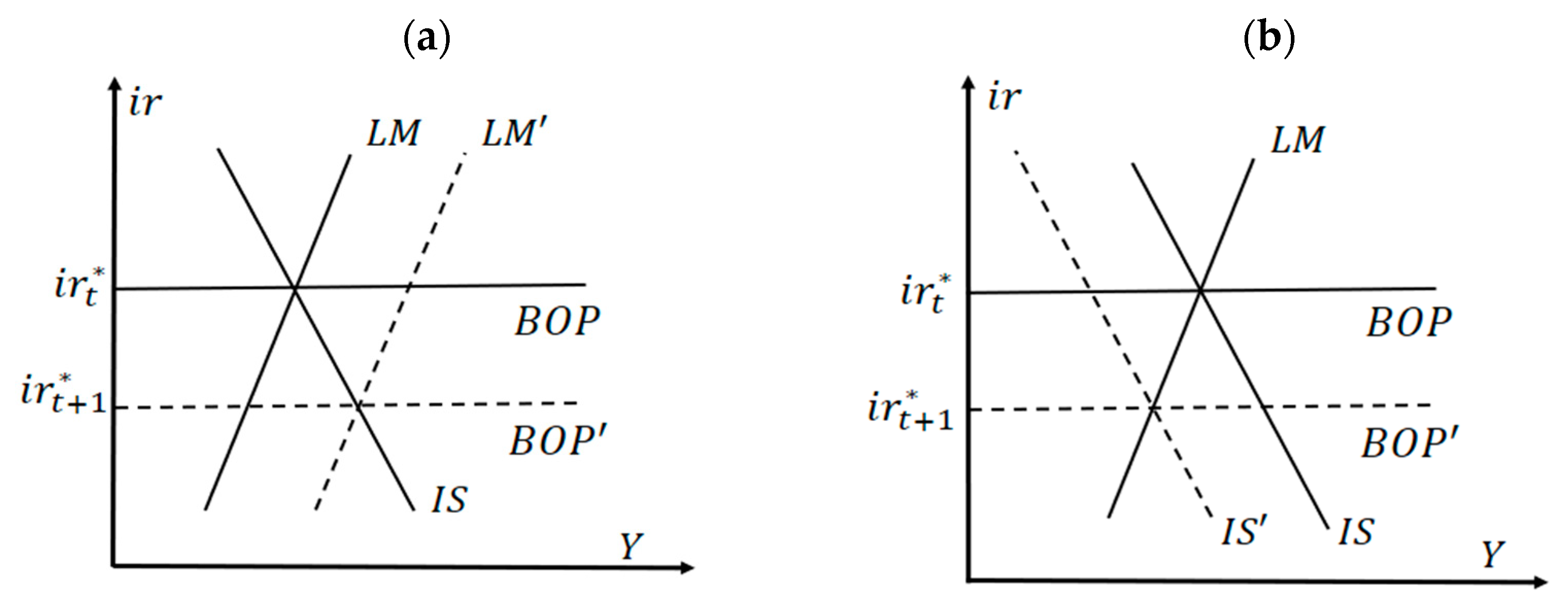
The impacts of capital flow on the significant national factors (output, inflation, and inventory prices) investigated in this research depend on the exchange rate regime. In the fixed exchange rate regime, balance in Equation (3) on the foreign exchange market is accomplished by providing cash to the recipient of the capital flows.

Figure 2a explain the fixed exchange rate regime. If the global interest rate decrease under the domestic rate $i{r}_{t+1}^{*}$, capital inflow occurs to take advantage of this opportunity. This would appreciate home currency. Central Bank sell of its foreign currency reserves to offset this capital inflow. Domestic interest rates have adapted to global interest rates at the new equilibrium point in this system. The decrease of the money supply would shifts the LM curve to the right until the domestic interest rate equal with global interest rate $i{r}_t^{*}$. Figure 2b explain the floating exchange rate regime. Conversely, if currency appreciation determines the exchange rate, it has a tendency to decrease the competitiveness of export products. The decrease of the global interest rate $i{r}_{t+1}^{*}$ will cause downward pressure on the local interest rate. The pressure will move as the domestic rate closes to the global rate. When negative differential occurs ($i{r}_{t+1}^{*}-i{r}_t^{*}<0$), the central bank holds no monetary expansion. When LM Curve holds constant, capital will flow in of the domestic economy. This appreciation the domestic currency will decrease the net export. Decreasing net export shifts the IS to the left until the domestic interest rate equal to the global rate ($i{r}_t=i{r}_t^{*}$).

In this case, liquidity in the global safe asset market is identified by the monetary aggregate $m_t^{*}$, whereas liquidity in the global risk asset market is projected by the risk premium $r{p}_t$. The global economy is modeled according to the following equations:

$$Y_t^{*}=E_t{Y}_{t+1}^{*}-\frac{1}{\rho }\left(i{r}_t^{*}-E_t\mathsf{\Delta }{P}_{t+1}^{*}\right)$$

(4)

$$\epsilon \left(M_t^{*}-P_t^{*}\right)=-\frac{\beta }{1-\beta }i{r}_t^{*}+\rho Y_t^{*}$$

(5)

$$\mathsf{\Delta }{P}_t^{*}=\beta E_t\mathsf{\Delta }{P}_{t+1}^{*}+\rho \kappa Y_t^{*}$$

(6)

where $P_t^{*}$ is the global price level, $Y_t^{*}$ is the global GDP, and $i{r}_t^{*}$ is the global interest rate. Equation (5) describes equilibrium in the money market (LM), Equation (4) in this case describes equilibrium in the goods market (IS), while Equation (6) is a reflection of the tradeoff between output and inflation (Phillips curve). Exogenous shocks affect liquidity in the global safe asset market, where $M_t^{*}$ increases permanently. The output and rate of domestic inflation for a small open economy are modeled as a function of past values, current values, and expectations of future value of global GDP ($Y^{*}$), nominal exchange rate (ER), real exchange rate (Q), global inflation ($\mathsf{\Delta }{P}^{*}$), and domestic interest rate (ir), as follows:

$$Y=f\left(Q,Y^{*},\mathsf{\Delta }P,ir\right)\mathrm{Where}\frac{\partial Y}{\partial Q}>0;\frac{\partial Y}{\partial Y^{*}}>0;\frac{\partial Y}{\partial \left(\mathsf{\Delta }P\right)}>0;\frac{\partial Y}{\partial ir}<0$$

(7)

$$\mathsf{\Delta }P=f\left(\mathsf{\Delta }S,\mathsf{\Delta }{P}^{*},\mathsf{\Delta }Y\right)\mathrm{Where}\frac{\partial \left(\mathsf{\Delta }P\right)}{\partial \left(\mathsf{\Delta }\mathrm{E}\right)}>0;\frac{\partial \left(\mathsf{\Delta }P\right)}{\partial \left(\mathsf{\Delta }{P}^{*}\right)}>0;\frac{\partial \left(\mathsf{\Delta }P\right)}{\partial \left(\mathsf{\Delta }Y\right)}>0$$

(8)

The ER is assumed to move in accordance with the uncovered interest rate parity, i.e.,:

$$E_t\mathsf{\Delta }E{R}_{t+1}=i{r}_t-i{r}_t^{*}+r{p}_t$$

(9)

The solution to this domestic model is determined by the rate function $i{r}_t$. In this case, one assumes that the central bank has a degree of monetary independence γ. Thus, interest rate movements will partially follow the domestic targets, which follow the Taylor rule:

$$i{r}_t=\gamma \left[\overline{i}+\varphi \left(Y_t-\overline{Y}\right)+\phi \left(\mathsf{\Delta }{P}_t-\overline{\mathsf{\Delta }P}\right)\right]+\left(1-\gamma \right)i{r}_t^{*}$$

(10)

Equation (10) assumes that domestic monetary policy plays a significant role in determining the spillover effect of global liquidity. 0 < γ < 1 implies that liquidity expansion in the global safe asset market will have a positive effect on inflation, GDP, and domestic asset prices. The appreciation of the exchange rate can offset a rise in inflation, up to a point. The decrease in $r{p}_t$ and expansion of liquidity in the global risk asset market will have a spillover effect in a similar direction.

The theoretical description of the relationship between variables in the TVAR model is explained as follows: Equation (7) explains the impact of global GDP ($Y^{*}$), real exchange rate (Q), domestic inflation ($\mathsf{\Delta }P$), global inflation ($\mathsf{\Delta }{P}^{*}$), and domestic interest rate (ir) on domestic GDP ($Y$). Equation (8) explains the impact of nominal exchange rate (ER) and global inflation ($\mathsf{\Delta }{P}^{*}$) on domestic inflation ($\mathsf{\Delta }P$). Equation (5) explains the role of the global price level in determining the level of global liquidity. Equations (4) and (6) explain the dynamic relationship between global inflation ($\mathsf{\Delta }{P}^{*}$) and global GDP ($Y^{*}$).

Equation above show that global GDP ($Y^{*})$, domestic GDP ($Y$), global inflation ($\mathsf{\Delta }{P}^{*}$), and domestic inflation ($\mathsf{\Delta }P)$ dynamically influence one another. The world commodity price P* is included because it plays an important role in determining world exchange rates and inflation. Endogenous and dynamic interrelationships were applied through the VAR model. If the VAR model assumes the impact of the invariant variable, TVAR assumes the impact between the variant variables, depending on the global economic regime.

Literature Review

Brana et al. (2012) discovered the structural breaks in this excess liquidity growth in 1995, wherein subsequent periods showed a higher and more persistent rate of growth. Monetary aggregate growth has been decoupled from global output growth, leading to what is known as excess liquidity.

Previous studies (Brana et al. 2012; Belke et al. 2010a; Sousa and Zaghini 2007) showed that global liquidity positively influenced short-term output. Psalida and Sun (2011) also observed positive effects on the credit gap, indicating the role of credit channels in the transmission of global liquidity impacts. Meanwhile, Matsumoto (2011) found that the rising levels of global risk aversion, as measured by the CBOE volatility index (VOX index), have a negative effect on output in various developed and emerging countries. Research conducted by Sousa and Zaghini (2007) and Belke et al. (2010b) found that global liquidity expansion boosted inflation both at the global level and at the level of individual countries/groups of countries. This is also consistent with the findings of Ciccarelli and Mojon (2010) that there is a robust error-correction mechanism between domestic inflation and global inflation.

3. Methodology

Estimation Methods

According to Galih and Safuan (2018), there is a simultaneous and dynamic two-way relationship between inflation and economic growth. This relationship experiences a regime change, to be positive or negative, which is suspected to occur based on certain factors within a country. These factors vary between economies because each country has unequal economic characteristics, e.g., policy, ideological, geographic, etc. Therefore, additional variables are needed in order to capture the relationship between inflation and economic growth. In our opinion, it is important to capture the differences between these characteristics.

We compiled a threshold vector autoregression (TVAR) model involving liquidity indicators in the global market, indicators of Indonesian macroeconomic and financial variables (or peers), and other global variables as controls. TVAR is an appropriate method of identifying the nonlinear effects of exogenous shock on a system of mutually endogenous variables, and is therefore widely used in empirical studies of macroeconomics in general, and of global liquidity in particular. A complete description of the TVAR model is given in the work of Ekananda (2017) for the research of the interaction of banking variables using TVAR. Briefly, the TVAR framework is described as follows: a system of structural equations beginning with Equation (11), where $Y_t$ is a vector of n endogenous variables, $B\left(L\right)$ is the matrix $n X n$ lag operator for $Y_t$, and $e_t$ is error terms:

$$\mathsf{\Gamma }{Y}_t=B\left(L\right)Y_t+e_t$$

(11)

The reduced form (Equation (12)) is obtained by multiplying Equation (11) by the inverse of Γ, which is the parameter of the contemporary relation for $Y_t$,. Equation (11) is changed in order to obtain the endogenous variable equation entirely on the left-hand side and the endogenous variable entirely on the right-hand side.

$$Y_t={\mathsf{\Gamma }}^{-1}B\left(L\right)Y_t+{\mathsf{\Gamma }}^{-1}{e}_t$$

$$Y_t=B^{*}\left(L\right)Y_t+u_t$$

(12)

This system of Equation (12) can be expressed in terms of a moving-average vector:

$$\left(I-B^{*}\left(L\right)\right)Y_t=u_t$$

$$Y_t=\mathsf{\Psi }{u}_t$$

(13)

where $\mathsf{\Psi }={\left(I-B^{*}\left(L\right)\right)}^{-1}$. The matrix $\mathsf{\Psi }$ is the impulse response function (IRF) of the reduced-form model, but the reduced-form $u_t$ error term, in this case, is not economically meaningful. To identify the IRF against structural error or innovation t, the PVAR method applies two types of restriction to solve Equation (14):

$${\mathsf{\Gamma }}^{-1}{e}_t=u_t$$

(14)

The first restriction is based on the assumption that structural innovation is orthogonal, or uncorrelated between variables. This allows the normalization of the variance–covariance matrix ${\mathsf{\Sigma }}_e$ into an identity matrix, giving the following equation:

$${\mathsf{\Gamma }}^{-1}{\mathsf{\Sigma }}_e{\mathsf{\Gamma }}^{-1^{\prime }}={\mathsf{\Sigma }}_u$$

(15)

In this case, we applied Cholesky decomposition, which makes ${\mathsf{\Gamma }}^{-1}$ an orthogonal matrix, since this form of restriction guarantees the fulfillment of the rank condition regardless of the exogeneity block restriction that we apply to the lag terms (Rubio-Ramirez et al. 2010). An appropriate variable is a crucial factor in ensuring the inference validity of this estimate. The TVAR model is a threshold model developed by Tong (1983), which is used to capture nonlinear phenomena in multivariate time series. The linear VAR model captures only linear impacts for all levels of data. The economy always makes adjustments at a certain economic level. The TVAR model calculates the threshold value of the economic variable used as an exogenous component. The TVAR model produces an efficient regression because its parameters are more flexible according to the variable threshold level. The hope is that TVAR regression results have a smaller residual sum of squares value.

Different thresholds can be implemented in the model. This research used two regimes to demonstrate high- and low-regime situations, dividing the variables into two regimes so that the differences were easier to investigate. The reason for implementing a threshold is because changes in impact can be seen in certain economic situations. In simple regression, the impact of independent variables is considered fixed for various economic situations. We used a dummy variable to explain the effects of two distinct circumstances.

We use TVAR developed by Balke (2000). The TVAR model consists of the dependent variables lag and threshold, and can be shown as follows:

$$Y_t=D^1+A^1{Y}_t+B^1\left(L\right)Y_{t-1}+\left(D^2+A^2{Y}_t+B^2\left(L\right)Y_{t-1}\right)I_t[C_{t-d}>\gamma ]e_t$$

(16)

where $Y_t$ is the vector of the endogenous variable, and $I_t[C_{t-d}>\gamma ]$ is an indicator function that has a value of 1 when the lag threshold $C_t$ is lower than critical threshold γ, and 0 otherwise. The model identifies two separate regimes based on $C_{t-d}$, where d is the time lag relative to $\gamma$, which is endogenously determined by the system. If $I_t[C_{t-d}>\gamma ]$ is 0, then the estimation result is $D^1+A^1+B^1\left(L\right)$, whereas if $I_t[C_{t-d}>\gamma ]$ is 1, then the estimation becomes $D^1+D^2+A^1+A^2+B^1\left(L\right)+B^2\left(L\right)$. The existence of this asymmetry can be identified by the threshold vector constant term D, and the different matrix coefficients A and B(L) in each regime.

In the analysis process, TVAR is different from the general VAR method. The difference between the two methods is the existence of a threshold variable. TVAR calculates nonlinear IRF (impulse response function), which captures variable responses to the shock in different regimes. Researchers formed the TVAR model through several testing stages—namely, stationary testing, stability testing, determination of optimal lag, and co-integration testing. Further analysis of the TVAR or VAR models includes IRF and FEVD analysis. Particularly for TVAR, threshold estimation and nonlinear IRF analysis were performed to determine responses in terms of endogenous variables in the event of certain shock variables.

Due to its theoretical nature, the selection of variables and the proper determination of restriction are the most crucial factors in TVAR estimation. We list the variables in this research as follows:

$$\left[\begin{array}{cc}{\mathrm{gdp}}_{\mathrm{t}}^{\mathrm{w}}& \begin{array}{ccc}{\mathrm{infl}}_{\mathrm{t}}^{\mathrm{w}}& {\mathrm{comm}}_{\mathrm{t}}^{\mathrm{w}}& \begin{array}{cc}{\mathrm{gdp}}_{\mathrm{t}}^{\mathrm{ind}}& {\inf }_{\mathrm{t}}^{\mathrm{ind}}\end{array}\end{array}\end{array}\right]$$

(17)

where ${\mathrm{gdp}}_{\mathrm{t}}^{\mathrm{w}}$ is the real world GDP, ${\inf }_{\mathrm{t}}^{\mathrm{ind}}$ is the consumer price level (Indonesian), ${\mathrm{infl}}_{\mathrm{t}}^{\mathrm{w}}$ is global inflation using the world GDP deflator, ${\mathrm{comm}}_{\mathrm{t}}^{\mathrm{w}}$ is the global commodity price level, and ${\mathrm{gdp}}_{\mathrm{t}}^{\mathrm{ind}}$ is the real GDP of Indonesia. This sequence is based on theories and literature on global shock transmission. The global variable block is placed before the domestic variable blocks in order to avoid the contemporary effects of domestic variables on global variables, in accordance with the assumption that shock in a small open economy such as Indonesia cannot affect global economic conditions.

The output is placed at the beginning, in accordance with the findings of Christiano et al. (1998) that output and inflation only react to liquidity shock after a certain lag. Inflation comes after output but before the liquidity/monetary and asset prices (commodities, stocks), according to the assumption of nominal rigidity in the Keynesian/neo-Keynesian model, where the price level adjusts only to shocks on other variables after a certain lag (Williamson and Wright 2010). Meanwhile, the prices of assets such as commodities, currencies (exchange rates), and stocks are placed most recently on their respective blocks, in accordance with the efficient market hypothesis, in which financial markets can react instantly to new information that may shape expectations of the asset price (Malkiel 2003). The following are the model specifications in this research, where the model country used was Indonesia. In this model, it is assumed that contemporaneous effects follow Cholesky’s rules, wherein the order is based on Balke (2000). The general equation of TVAR is:

$$Y_t=\left(B_1{Y}_t+B_2\left(L\right)Y_{t-1}+B_3\left(L\right)Y_{t-2}\right)I_t\left(C_{t-d}>\gamma \right)+u$$

(18)

The complete equation of TVAR is as follows:

$$\left[\begin{array}{c}{\mathrm{gdp}}_{\mathrm{t}}^{\mathrm{w}}\\ {\mathrm{infl}}_{\mathrm{t}}^{\mathrm{w}}\\ {\mathrm{comm}}_{\mathrm{t}}^{\mathrm{w}}\\ {\mathrm{gdp}}_{\mathrm{t}}^{\mathrm{ind}}\\ {\inf }_{\mathrm{t}}^{\mathrm{ind}}\end{array}\right]=\left(\left[\begin{array}{c}\\ {\mathrm{a}}_1\\ {\mathrm{a}}_2\\ {\mathrm{a}}_4\\ {\mathrm{a}}_7\end{array}\begin{array}{c}\\ \\ {\mathrm{a}}_3\\ {\mathrm{a}}_5\\ {\mathrm{a}}_8\end{array}\begin{array}{c}\\ \\ \\ {\mathrm{a}}_6\\ {\mathrm{a}}_9\end{array}\begin{array}{c}\\ \\ \\ \\ {\mathrm{a}}_{10}\end{array}\begin{array}{c}\\ \\ \\ \\ \end{array}\right]\left[\begin{array}{c}{\mathrm{gdp}}_{\mathrm{t}}^{\mathrm{w}}\\ {\mathrm{infl}}_{\mathrm{t}}^{\mathrm{w}}\\ {\mathrm{comm}}_{\mathrm{t}}^{\mathrm{w}}\\ {\mathrm{gdp}}_{\mathrm{t}}^{\mathrm{ind}}\\ {\inf }_{\mathrm{t}}^{\mathrm{ind}}\end{array}\right]+{\sum }_{\mathrm{l}=1}^{\mathrm{p}}\right[\begin{array}{c}{\mathrm{b}}_{11}\\ {\mathrm{b}}_{21}\\ {\mathrm{b}}_{31}\\ {\mathrm{b}}_{41}\\ {\mathrm{b}}_{51}\end{array}\begin{array}{c}{\mathrm{b}}_{12}\\ {\mathrm{b}}_{22}\\ {\mathrm{b}}_{32}\\ {\mathrm{b}}_{42}\\ {\mathrm{b}}_{52}\end{array}\begin{array}{c}{\mathrm{b}}_{13}\\ {\mathrm{b}}_{23}\\ {\mathrm{b}}_{33}\\ {\mathrm{b}}_{43}\\ {\mathrm{b}}_{53}\end{array}\begin{array}{c}{\mathrm{b}}_{14}\\ {\mathrm{b}}_{24}\\ {\mathrm{b}}_{34}\\ {\mathrm{b}}_{44}\\ {\mathrm{b}}_{54}\end{array}\begin{array}{c}{\mathrm{b}}_{15}\\ {\mathrm{b}}_{25}\\ {\mathrm{b}}_{35}\\ {\mathrm{b}}_{45}\\ {\mathrm{b}}_{55}\end{array}\left]\left[\begin{array}{c}{\mathrm{gdp}}_{\mathrm{t}-\mathrm{l}}^{\mathrm{w}}\\ {\mathrm{infl}}_{\mathrm{t}-\mathrm{l}}^{\mathrm{w}}\\ {\mathrm{comm}}_{\mathrm{t}-\mathrm{l}}^{\mathrm{w}}\\ {\mathrm{gdp}}_{\mathrm{t}-\mathrm{l}}^{\mathrm{ind}}\\ {\inf }_{\mathrm{t}-\mathrm{l}}^{\mathrm{ind}}\end{array}\right]\right)I_t\left(C_{t-d}>\gamma \right)+u_t$$

(19)

where $C_{t-d}$ is the lag threshold variable (−1); $I_t$ is a function indicator that has a value of 1 if the lag of the threshold variable is lower compared to the critical value threshold $\gamma$, and 0 otherwise; B₁(L), B₂(L), and B₃(L) are the lag polynomial matrices; and $u_t$ is an error term. The structure of the orthogonal Cholesky matrix $B_1$ shows the contemporaneous parameter to the right of the equation. This research assumes that some variables have endogenous and dynamic relationships. This dynamic relationship experienced a regime change due to the nonlinear relationships that occur in the threshold $C_t$ or lag (−1) variables at various points. The selection of threshold variables in the model refers to the work of Chowdhury and Ham (2009). The selected thresholds are the real-world output ${\mathrm{gdp}}_{\mathrm{t}-1}^{\mathrm{w}}$, world commodity index ${\mathrm{comm}}_{\mathrm{t}-1}^{\mathrm{w}}$, and world inflation ${\inf }_{\mathrm{t}-1}^{\mathrm{w}}$. This variable plays an exogenous role, affecting the economy in Indonesia.

This model has two regimes due to the existence of the threshold, where the inflation rate is below the threshold limit; hence, the economic conditions are in the lower regime; when the inflation rate is above the threshold, this means that the economic condition is in the upper regime (Galih and Safuan 2018). The selection of threshold variables is based on the role of past inflation rates in determining the actual or current inflation targets at that time.

The nonlinear relationship refers to the behavior change of some variables over a period of time, caused by certain factors or economic conditions (Suryanto et al. 2020). These factors allegedly occur due to changes in aggregate supply and demand, changes in wage rates, changes in inflation expectations, monetary crisis, or new government policies and central bank policies. The relationship between inflation and economic growth that occurs in an economy can also be affected by other conditions.

4. Results and Discussion

The selected domestic variables in this research were real GDP (output), Indonesian inflation, and world inflation.

All of the data incorporated in this research were obtained from The Central Bureau of Statistics (BPS), Bloomberg LP, and International Financial Statistics (IFS) databases (

Table 1. List of variables.

Variable	Sources
Global real output (${\mathrm{gdp}}_{\mathrm{t}}^{\mathrm{w}}$)
Global deflator GDP (${\mathrm{infl}}_{\mathrm{t}}^{\mathrm{w}})$	IFS	Year-on-year %
Global commodity price index SandP* (${\mathrm{comm}}_{\mathrm{t}}^{\mathrm{w}})$	Bloomberg
Real output Indonesia (${\mathrm{gdp}}_{\mathrm{t}}^{\mathrm{ind}}$)	BPS, IFS	Base year 2010
Consumer price index (CPI) ${\inf }_{\mathrm{t}}^{\mathrm{ind}}$	IFS	Base year 2010

), all of which employed logarithms except for interest rate, global GDP, and global GDP deflator. We applied the Census X12 procedure to the leveled information to minimize the seasonal impact of the information, and used a year-on-year differential for the first differential. This study uses quarterly data between 1996:Q1 to 2018:Q4.

Table 2. Data description.

Variable	$\mathbf{g}\mathbf{d}{\mathbf{p}}_{\mathbf{t}}^{\mathbf{w}}$	$\mathbf{i}\mathbf{n}\mathbf{f}{\mathbf{l}}_{\mathbf{t}}^{\mathbf{w}}$	$\mathbf{c}\mathbf{o}\mathbf{m}{\mathbf{m}}_{\mathbf{t}}^{\mathbf{w}}$	$\mathbf{g}\mathbf{d}{\mathbf{p}}_{\mathbf{t}}^{\mathbf{i}\mathbf{n}\mathbf{d}}$	$\mathbf{i}\mathbf{n}{\mathbf{f}}_{\mathbf{t}}^{\mathbf{i}\mathbf{n}\mathbf{d}}$
Mean	0.033	0.073	0.048	0.042	0.097
Median	0.033	0.049	0.027	0.056	0.076
Maximum	0.058	0.213	0.490	0.102	0.579
Minimum	−0.019	0.010	−0.633	−0.202	−0.006
Std. Dev.	0.014	0.058	0.215	0.049	0.096
Skewness	−0.986	1.377	−0.668	−3.147	3.592
Kurtosis	5.323	3.433	4.016	13.765	16.604
Jarque–Bera	35.598	29.802	10.805	596.100	907.286
Probability	0.000	0.000	0.005	0.000	0.000
Observations	92	92	92	92	92

explains the descriptive statistics covering mean, median, and maximum values, etc. To fundamentally determine the normality, as described by Brys et al. (2004), the ranges of skewness and kurtosis of these relevant data were within the range of −2.58 to +2.58, implying that the z-scores performed in a normal manner. The large Jarque–Bera values mean that the null hypothesis of normality was rejected at the 5% significance level, indicating that the ${\mathrm{gdp}}_{\mathrm{t}}^{\mathrm{w}}$, ${\mathrm{infl}}_{\mathrm{t}}^{\mathrm{w}}$, ${\mathrm{comm}}_{\mathrm{t}}^{\mathrm{w}}$, ${\mathrm{gdp}}_{\mathrm{t}}^{\mathrm{ind}}$, and ${\inf }_{\mathrm{t}}^{\mathrm{ind}}$ have a non-normal distribution. The ${\mathrm{gdp}}_{\mathrm{t}}^{\mathrm{w}}$, ${\mathrm{infl}}_{\mathrm{t}}^{\mathrm{w}}$, ${\mathrm{comm}}_{\mathrm{t}}^{\mathrm{w}}$, ${\mathrm{gdp}}_{\mathrm{t}}^{\mathrm{ind}}$, and ${\inf }_{\mathrm{t}}^{\mathrm{ind}}$ series fluctuate in accordance with the impact of global economic crises.

Table 3. Unit root test.

Variable	1st Difference
Global real output, ${\mathrm{gdp}}_{\mathrm{t}}^{\mathrm{w}}$	−3.571 ***
Global deflator GDP, ${\mathrm{infl}}_{\mathrm{t}}^{\mathrm{w}}$	−1.672
Global commodity price index, ${\mathrm{comm}}_{\mathrm{t}}^{\mathrm{w}}$	−4.016 ***
Real GDP, Indonesia, ${\mathrm{gdp}}_{\mathrm{t}}^{\mathrm{ind}}$	−3.059 **
CPI, Indonesia, ${\inf }_{\mathrm{t}}^{\mathrm{ind}}$	−3.415 **

Phillips and Perron test at lag:1, with intercept and without trend. Level of significance: ** 95%, *** 99%.

shows that the majority of variables were incorporated in one order in this research (I (1)); some of them are covariance-stationary or trend-stationary at the national level (Ekananda 2016; Enders 2009). Especially for GDP and the global GDP deflator, the data obtained from IFS are a percentage of year-on-year growth, so root units at this level cannot be known. The hypothesis of a root unit is denied for global GDP growth, but cannot be denied for global GDP deflator growth.

To test the null hypothesis of linearity against the alternative of nonlinearity (t = 1, 2), where t indicates the threshold value, we used a multivariate extension of the linearity test by Hansen (1999), Hansen (2000), and Balke (2000) to test the statistical significance of the variable that is determined as the threshold indicator. The likelihood ratio (LR) test is formulated as follows: $L{R}_{01}=T\left(ln\left(det{\widehat{\mathsf{\Sigma }}}_0\right)-ln\left(det{\widehat{\mathsf{\Sigma }}}_1\right)\right)$, where ${\widehat{\mathsf{\Sigma }}}_0$, which is the estimated covariance matrix for the model, is related to the null hypothesis, and ${\widehat{\mathsf{\Sigma }}}_1$ is the estimated covariance matrix for the alternative hypothesis. We apply one threshold compared to applying more than one threshold. The division of two regimes in Indonesia was carried out by Galih and Safuan (2018) for Indonesian data.

Table 4. Likelihood ratio (LR) test.

LR Test for Linearity vs. One Threshold	$\mathbf{g}\mathbf{d}{\mathbf{p}}_{\mathbf{t}}^{\mathbf{w}}$	$\mathbf{i}\mathbf{n}\mathbf{f}{\mathbf{l}}_{\mathbf{t}}^{\mathbf{w}}$	$\mathbf{c}\mathbf{o}\mathbf{m}{\mathbf{m}}_{\mathbf{t}}^{\mathbf{w}}$
LR statistic	204.66862	257.21503	245.84690
p-value	0.0000	0.0000	0.0000
Estimated threshold	0.03200	0.10500	0.02300
Observations	Upper: 86 Lower: 5	Upper: 17 Lower: 74	Upper: 88 Lower: 3

summarizes the LR Test for linearity for 1. The null hypothesis is linearity. The LR test statistic shows that the null hypothesis is rejected for all tests. Therefore, ${\mathrm{gdp}}_{\mathrm{t}}^{\mathrm{w}}$, ${\mathrm{infl}}_{\mathrm{t}}^{\mathrm{w}}$, and ${\mathrm{comm}}_{\mathrm{t}}^{\mathrm{w}}$ can be used as thresholds for the VAR 1 threshold.

Table 5. Comparison of SSR threshold regression compared to linear regression.

Equations	SSR for No Threshold	SSR for Threshold GDPW at 0.03200
		Upper	Lower
GDP World (${\mathrm{gdp}}_{\mathrm{t}}^{\mathrm{w}}$)	0.0050132800	0.0038416049	3.69160 × 10−27
Infl World (${\mathrm{infl}}_{\mathrm{t}}^{\mathrm{w}}$)	0.0186676242	0.0180228736	4.47940 × 10−27
Comm World (${\mathrm{comm}}_{\mathrm{t}}^{\mathrm{w}}$)	1.6063031966	1.1363615102	5.28013 × 10−25
GDP Indonesia (${\mathrm{gdp}}_{\mathrm{t}}^{\mathrm{ind}}$)	0.0700752506	0.0696526329	1.01048 × 10−26
Infl Indonesia (${\inf }_{\mathrm{t}}^{\mathrm{ind}})$	0.1649023310	0.1607237144	2.74020 × 10−27
	Usable data: 91	Usable data: 86	Usable data: 5
		LR statistic: 204.66862 Degrees of freedom: 45

and

Table 6. SSR of equations at threshold world inflation and threshold world commodity index.

Equations	SSR for Threshold World Inflation at 0.10500		SSR for Threshold Comm at 0.02300
	Upper	Lower	Upper	Lower
GDP world (${\mathrm{gdp}}_{\mathrm{t}}^{\mathrm{w}}$)	0.0004696590	0.0028062174	0.0049166339	2.18237 × 10−26
Infl world (${\mathrm{infl}}_{\mathrm{t}}^{\mathrm{w}}$)	0.0003151193	0.0173336004	0.0184403660	4.69865 × 10−27
Comm world (${\mathrm{comm}}_{\mathrm{t}}^{\mathrm{w}}$)	0.1990931060	0.8375231994	1.5882522646	5.91141 × 10−26
GDP Indonesia (${\mathrm{gdp}}_{\mathrm{t}}^{\mathrm{ind}}$)	0.0247563092	0.0335070222	0.0699853918	7.08469 × 10−27
Infl Indonesia (${\inf }_{\mathrm{t}}^{\mathrm{ind}})$	0.0420768776	0.0440724164	0.1607748630	6.62446 × 10−27
	Usable data: 17	Usable data: 74	Usable data: 88	Usable data: 3
	LR statistic: 257.21503 Degrees of freedom: 45		LR statistic: 245.84690 Degrees of freedom: 45

shows the SSR values of the VAR (no threshold) model and the TVAR model, where the TVAR SSR value is lower than that of the VAR model. The TVAR model estimates generate a lower and more efficient SSR. We used RATS programming software to solve TVAR models (Enders and Doan 2014). Table 5 shows the lower SSR values using threshold regression compared with linear regression. Threshold regression generates a more robust and effective estimate. This can be demonstrated by assessing the values of the non-threshold and threshold sum of squared residuals (SSR). Based on the Hannan–Quinn (HQIC) and Schwarz Bayesian (SBIC) information criteria, the VAR model with maximum lag of 1 (VAR (1)) is the most appropriate for the complete model without lag restriction, while the same criteria applied for each block separately lead to the VAR (1) or VAR (2) models.

The study chose three threshold variables—namely, world GDP (${\mathrm{gdp}}_{\mathrm{t}}^{\mathrm{w}}$), world inflation (${\mathrm{infl}}_{\mathrm{t}}^{\mathrm{w}}$), and the world commodity index. World GDP rate (${\mathrm{gdp}}_{\mathrm{t}}^{\mathrm{w}}$) and world inflation rate (${\mathrm{infl}}_{\mathrm{t}}^{\mathrm{w}}$) play important roles in increasing Indonesia’s GDP and inflation. Applying GDP as a threshold was the basis of the research of Romyen et al. (2019). In general, if the GDP regime is higher, the behavior of small countries’ economic variables will be different if they are in a lower GDP regime. In conditions of higher world GDP, the response of Indonesian GDP is expected to be higher than in the event of lower world GDP. The use of world inflation and world price commodity index as thresholds is relevant to the research of Chowdhury and Ham (2009). In a high-world-GDP regime, the expectation is that Indonesian inflation will be high. In conditions of high world Inflation, the response of Indonesian GDP is expected to be higher than in the case of low world Inflation, due to the reaction of Indonesian production, which requires higher capital inflow and lower inflation. Likewise, Indonesian inflation will be high in the high-world-inflation regime, as a result of the response to capital outflows from Indonesia.

At a high world commodity index, the Indonesian economy will respond quickly by increasing commodity prices. At the low world commodity index, the Indonesian economy was slow to respond by lowering prices. Indonesia still needs imported raw materials for its production. Domestic prices must immediately follow the increase in world commodity indexes.

The second column shows SSR for the TVAR model with threshold GDPW. The model proposes a threshold GDPW value of 0.0320, which separates the VAR in the lower regime and upper regime. Upper and lower specifications are due to high and low statuses, and are more appropriate than crisis or non-crisis status. The crisis status must be relevant to the crisis status that the Indonesian monetary authority has issued.

The second column in Table 5 shows the SSR value of the TVAR model with inflation as the threshold. The world inflation threshold value is 0.1050. This value divides the inflation level into the upper regime and lower regime.

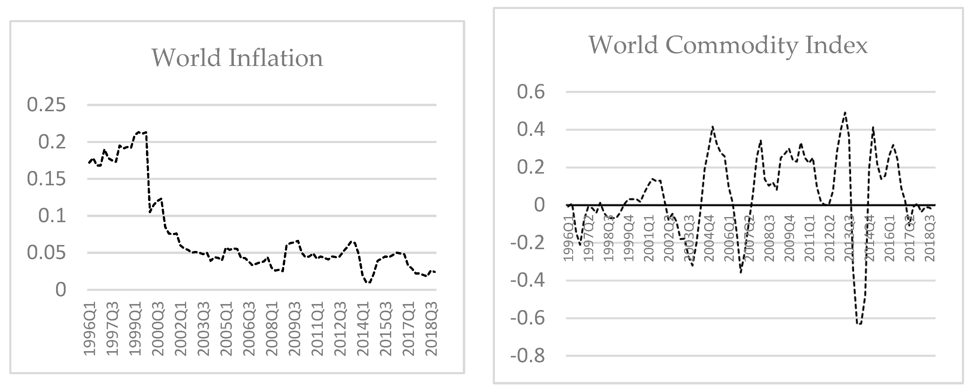
Column three in Table 6 shows the SSR value of the TVAR world commodity threshold index price; the threshold value is 0.023. This value divides the world commodity price index level into the upper regime and lower regime. Figure 3 shows the fluctuation data of the world inflation index and world commodity index. The division of inflation at the value of 0.105 is shown by the line that intersects the vertical scale of 0.105. The threshold occurred when the inflation index fell from 2002Q1 to 2018Q1. The inflation threshold divides the regime into two time-groups: before and after 2002Q1.

The division of the commodity index at 0.023 is shown at a value around zero (Figure 3, right panel). This value equally divides the commodity index into a regime of positive and negative indices. In general, the commodity index in the upper regime is positive.

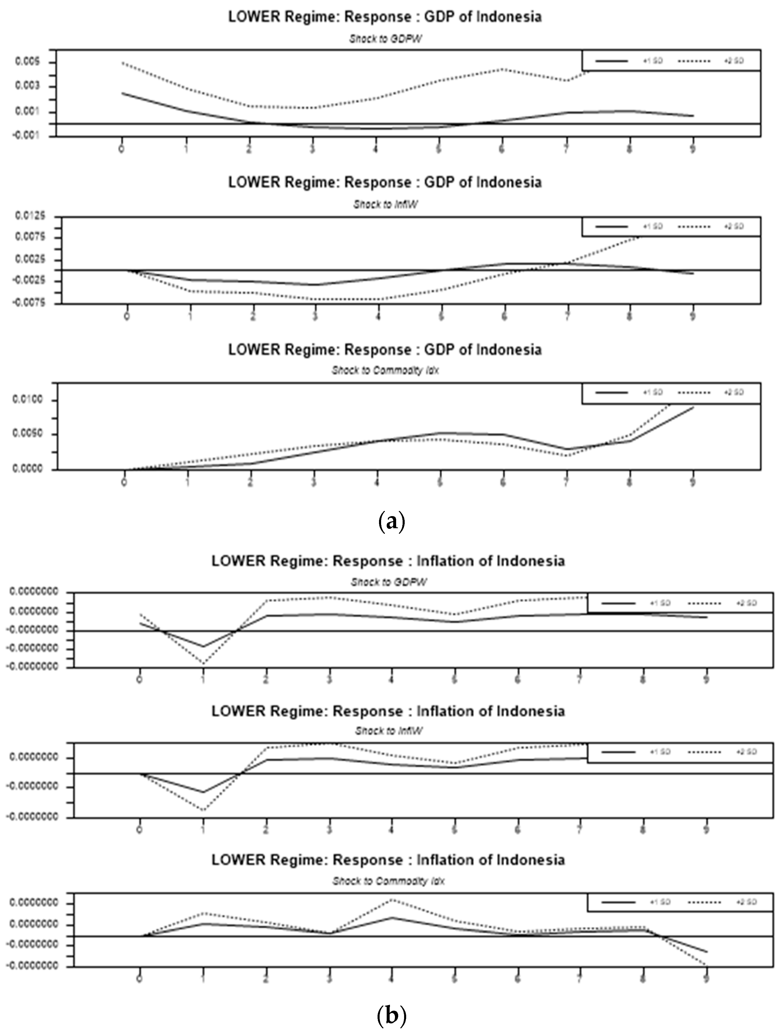
The IRF analysis of the TVAR model shows a different response if the same shock is applied to the variable shock propagator. The GDPW variable is significant as a threshold on the TVAR model’s security system. The GDPW threshold value of 0.023 indicates that the world GDP growth is above 2.3%, causing the difference in the VAR estimation equation. The VAR equations in the two regimes shape the responses of GDP and inflation in Indonesia differently. As usual in VAR analysis, the impulse response function is still a good analytical tool to estimate the response in the future to a sudden change of the variable propagator. The following discussion concerns the response of Indonesian GDP variables (${\mathrm{gdp}}_{\mathrm{t}}^{\mathrm{ind}}$) and Indonesian inflation to shock from world GDP propagator variables (${\mathrm{gdp}}_{\mathrm{t}}^{\mathrm{w}}$), world inflation (${\mathrm{gdp}}_{\mathrm{t}}^{\mathrm{w}}$), and the world commodity index (${\mathrm{infl}}_{\mathrm{t}}^{\mathrm{w}}$. ). Response variables are divided into upper and lower regimes according to the world’s GDP threshold (${\mathrm{gdp}}_{\mathrm{t}}^{\mathrm{w}}$), world inflation (${\mathrm{infl}}_{\mathrm{t}}^{\mathrm{w}}$), and world commodity index (${\mathrm{comm}}_{\mathrm{t}}^{\mathrm{w}}$). This study finds that Indonesia’s GDP and inflation responses are higher in a high world GDP situation, as a result of the conducive influence of the world economy that drives the Indonesian economy forward.

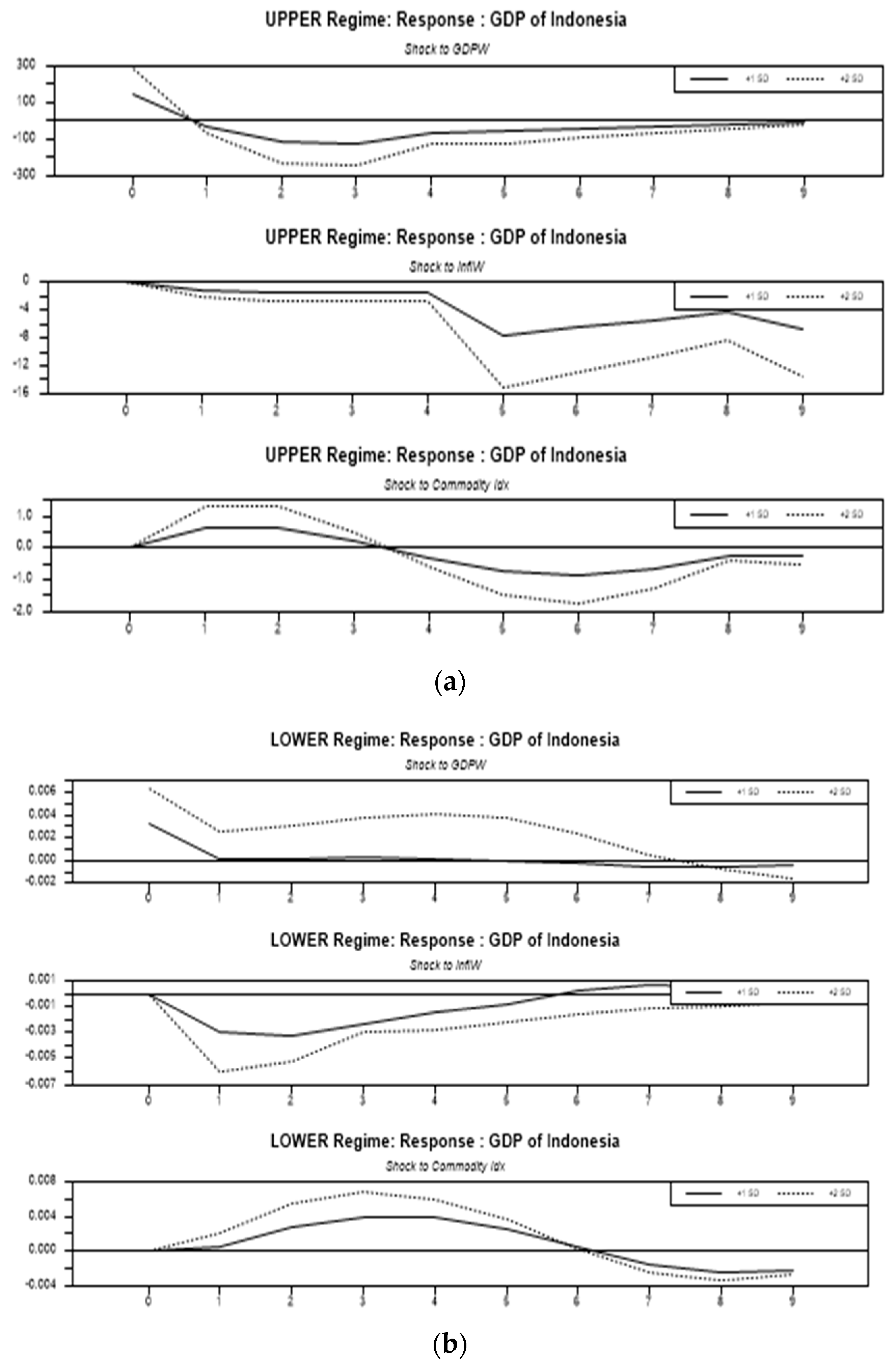
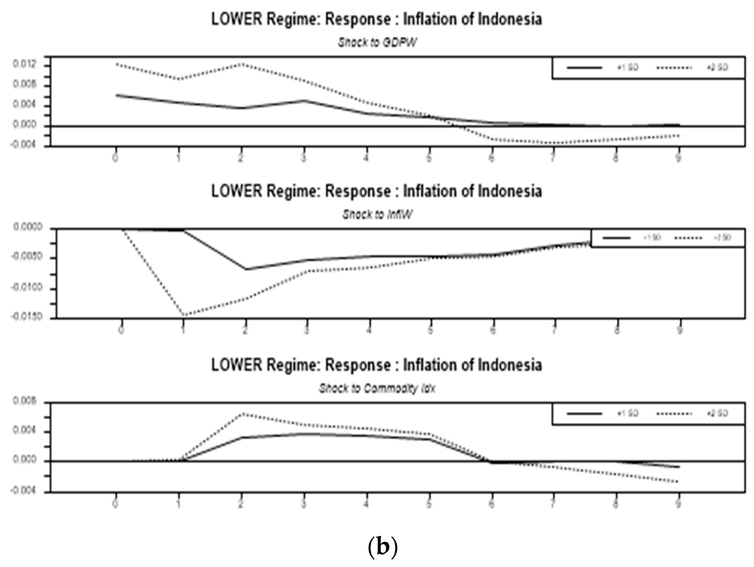
Figure 4a shows the response of the Indonesian GDP (${\mathrm{gdp}}_{\mathrm{t}}^{\mathrm{ind}}$) to the shock of world GDP propagators (${\mathrm{gdp}}_{\mathrm{t}}^{\mathrm{w}}$), world inflation (${\mathrm{infl}}_{\mathrm{t}}^{\mathrm{w}}$), and the world commodity index (${\mathrm{comm}}_{\mathrm{t}}^{\mathrm{w}}$), sequentially. In accordance with Cholesky’s orthogonalization, at high levels of world GDP, Indonesia’s GDP responded positively to world GDP shock; positive responses declined for the next 10 quarters. Indonesia’s GDP responded negatively to world inflation shocks; negative response continued until the 10th quarter. In the low regime, Indonesia’s GDP did not respond to the shock of world commodities. Indonesia’s GDP response caused by world GDP and world inflation was consistent with expectations (Galih and Safuan 2018).

Figure 4b shows Indonesia’s GDP response to the same shock propagators in the low-world-GDP situation, where Indonesia’s GDP does not respond to the shocks of world inflation, world commodities, and world GDP. In the case of shock propagators in all three variables, the low global economic situation cannot promote Indonesia’s GDP.

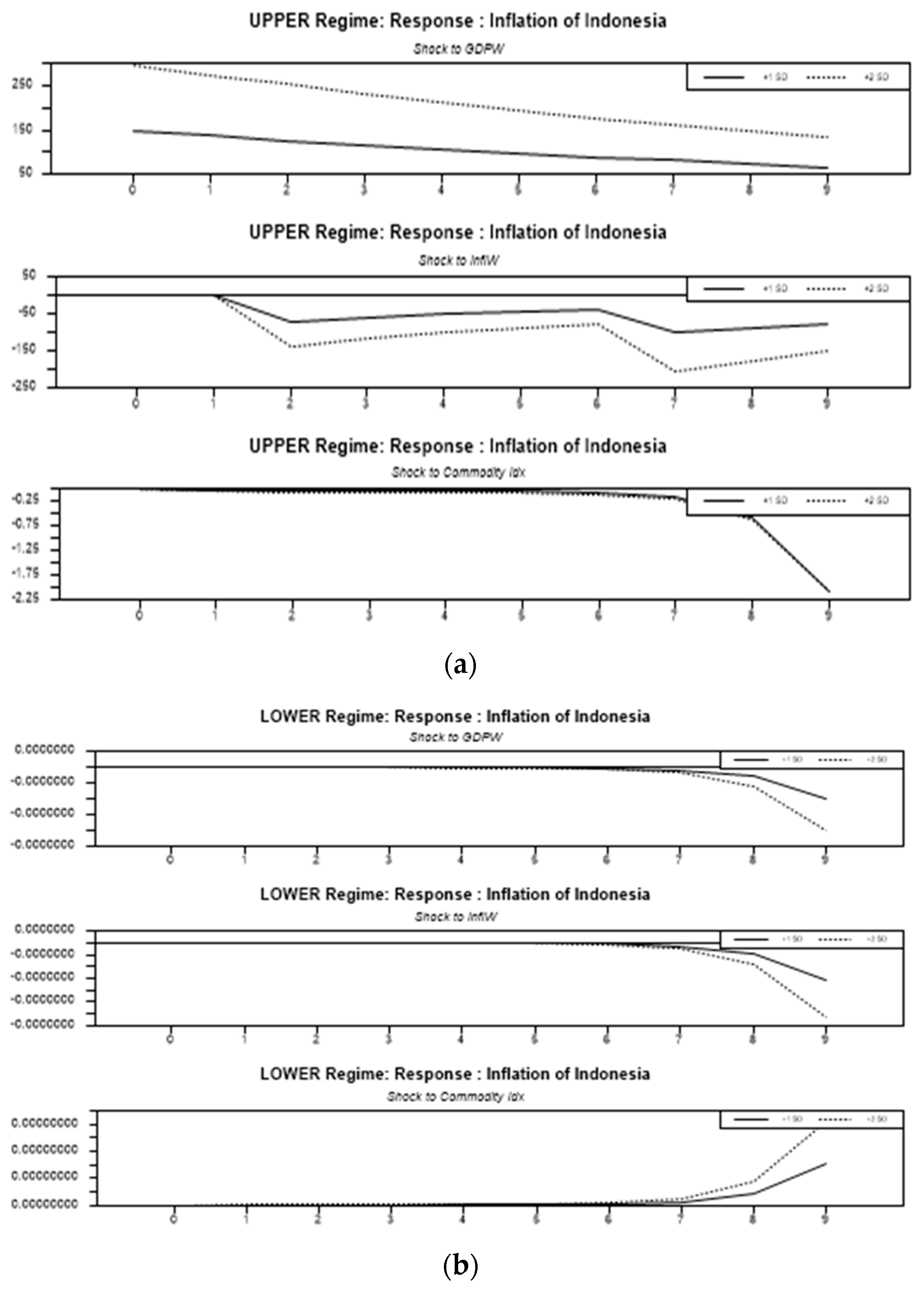
Figure 5a shows the response of Indonesia’s inflation ${\inf }_{\mathrm{t}}^{\mathrm{ind}}$ to the same shock propagator. The study applied the same Cholesky’s orthogonalization structure. The inflation response in the world’s high-GDP regime differs from Indonesia’s inflation response to the world’s low-GDP regime. At high world GDP, Indonesia’s inflation initially responded positively to the shock of world GDP; this response declined to its lowest in the third quarter. Similarly, Indonesia’s inflation responded negatively to the shock of world inflation. In contrast to the shock of world commodities, world inflation responded positively in the 2nd and 3rd quarters. Indonesia’s inflation response was stronger in the world’s low-GDP regime. This fact indicates that at low GDP, Indonesia’s inflation is more responsive than when the GDP regime is high. Some other authors have also explained this phenomenon (Gromb and Vayanos 2010).

Positive responses declined for the next 10 quarters. Indonesia’s GDP responded to negative shocks in world inflation; the negative response continued until the 10th quarter. In the low regime, Indonesia’s GDP did not respond to the shock of world commodities. Indonesia’s GDP response caused by world GDP and world inflation was consistent with expectations (Giese and Tuxen 2007).

In this study, we analyzed the variable response to the world inflation situation (${\mathrm{infl}}_{\mathrm{t}}^{\mathrm{w}}$) as the threshold. Threshold world inflation is 0.105. Figure 3 shows inflation in the initial period of high research, and then after 1996Q1 the inflation index is low. The threshold divides the data into two parts according to a clear time period. The analysis in this paper is only aimed at inflation response due to shock propagators. In the upper regime period, during the period of high world inflation. Figure 6a on the left shows Indonesia’s inflation will respond to the shock of global GDP positively. Inflation in Indonesia does not respond to shocks of world inflation. Indonesia’s inflation did not respond to the shock of world commodities at the beginning of the period, but in Q1, Indonesia’s inflation responded positively, but fell back until there was no response. This is because the inflation target applied in Indonesia is able to reduce the shocks of world inflation and world commodity prices.

Figure 6b shows Indonesia’s inflation response due to the shock propagators in the lower world inflation regime. The same phenomenon was observed as for the high regime, as described earlier. The magnitude of the response in the lower regime was greater. In the lower world inflation regime, inflation targeting policy is looser; thus, responses from various shock variables are more tolerated.

In the previous analysis, the threshold divides the world’s GDP into two regimes, enabling further studying of the world commodity prices (${\mathrm{comm}}_{\mathrm{t}}^{\mathrm{w}}$) as the threshold. The world commodity index reflects changes in the prices of commodities traded in the world. Changes in commodity prices lead to world inflation and changes in the flow of funds between countries. The decline in oil prices was able to undermine the world’s manufacturing industry and energy industry (Elizabeth et al. 2020). Increased commodity prices have not changed abruptly but, rather, through some adjustment processes following the global supply and demand mechanisms of commodities. Macroeconomic variables can capture the difference in response between the two regimes. The limit of change is reflected by the threshold value to be calculated in this study.

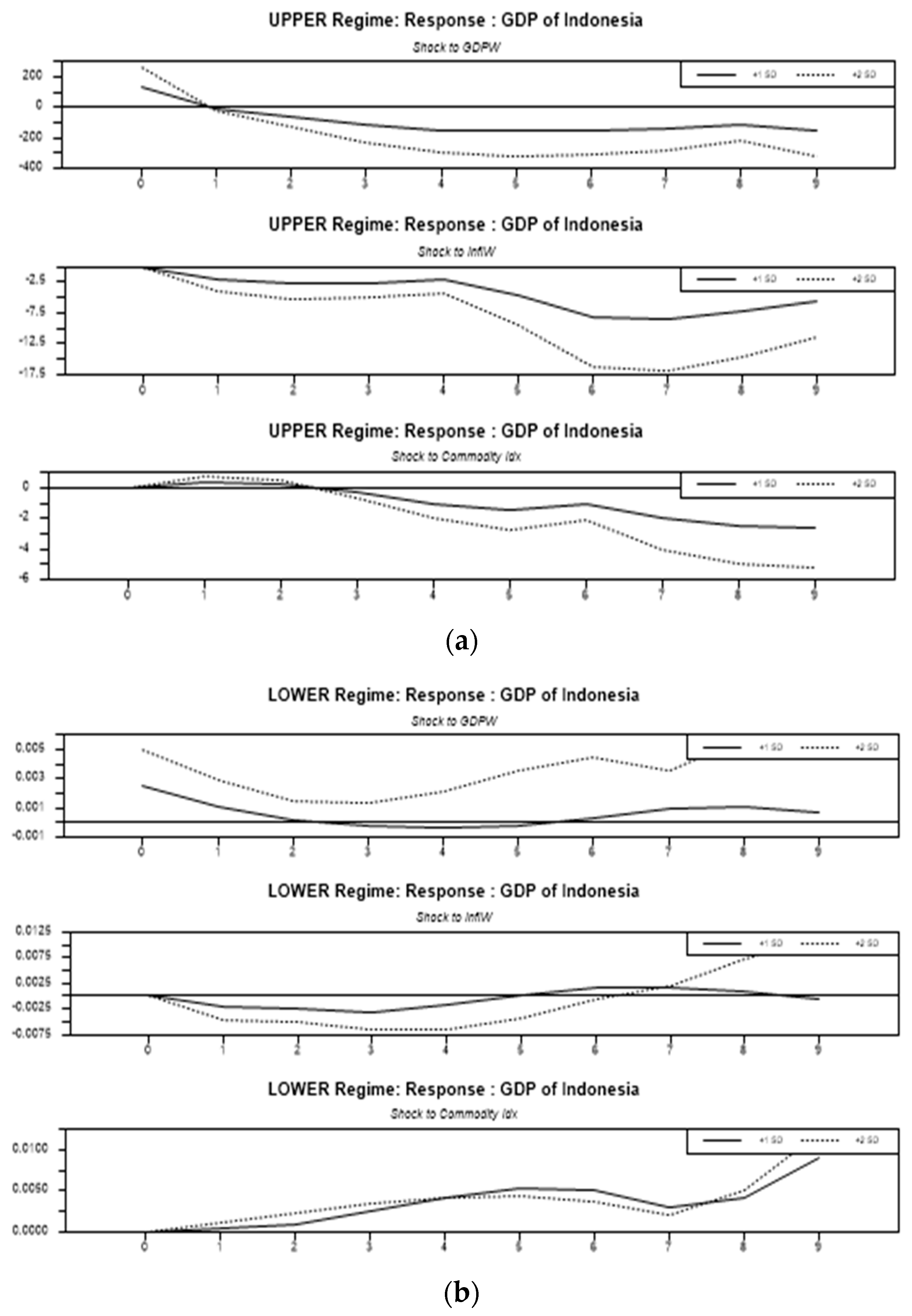
Threshold ${\mathrm{comm}}_{\mathrm{t}}^{\mathrm{w}}$ is measured at 0.02300. Figure 3 shows the fluctuation of the world commodity index, which is divided into two equal parts; some are positive, and others are negative. Figure 7a shows the response of Indonesian GDP to shock propagators. We can conclude that the upper regime is indicated by a positive index increase. When there is an increase in the world commodity index, Indonesia’s GDP experiences a bigger boost. This shows that Indonesia can increase its GDP when commodity prices in the world market increase. In the lower regime, the GDP response is weaker than in the upper regime.

The variable response in the lower regime shows different shapes. In general, the response variable in the lower regime is less responsive. The most obvious difference that occurred in Indonesia’s commodity response was due to world commodity shock. Indonesia’s commodity index responds positively to world shock commodities. This is consistent with the hypothesis that high world commodity prices will increase Indonesia’s inflation.

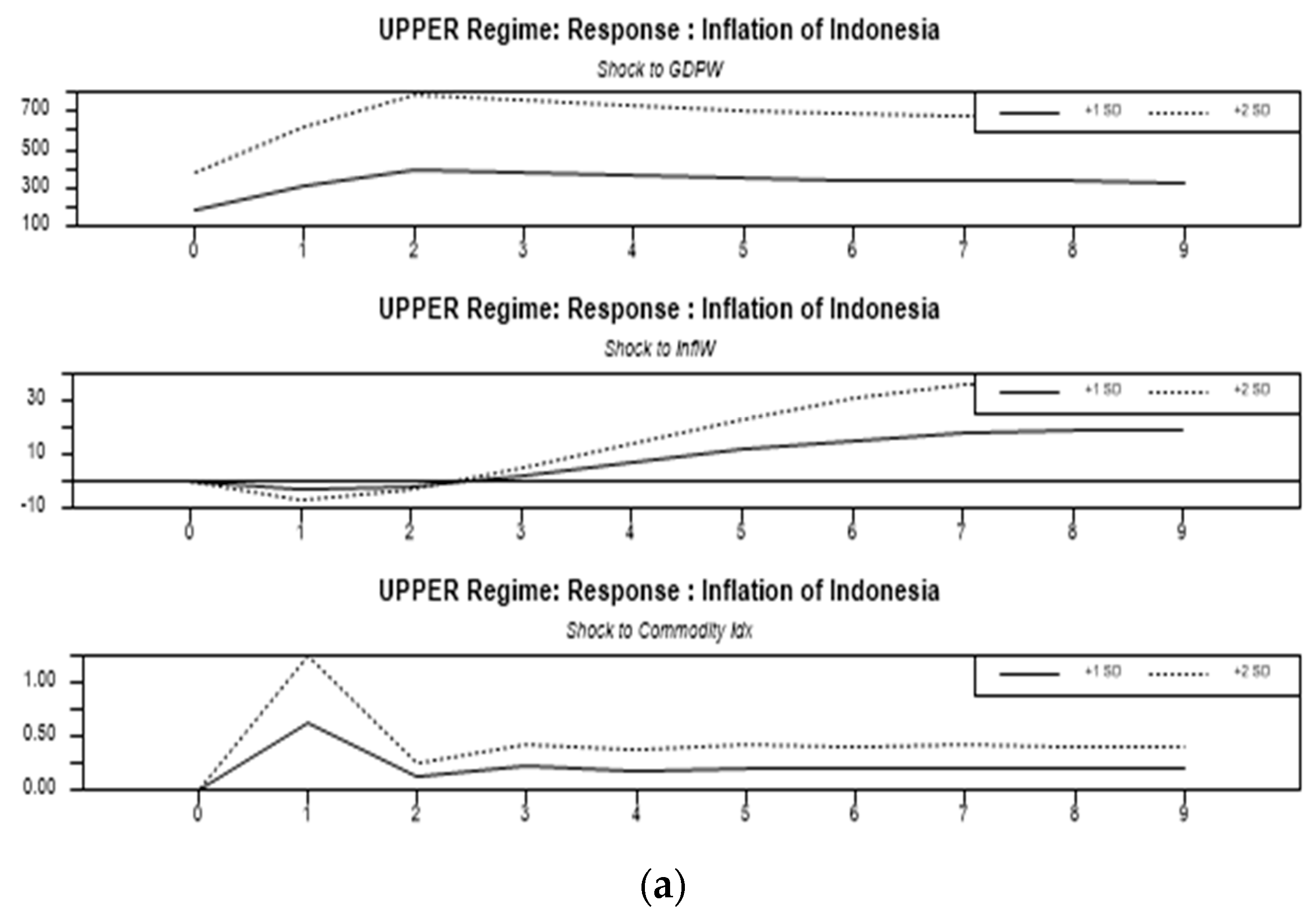
Figure 8 shows Indonesia’s inflation response due to shock propagators. Inflation response in the upper regime is different compared to the lower regime. In the upper regime, Indonesia’s inflation is positive at the beginning of world GDP shock (${\mathrm{gdp}}_{\mathrm{t}}^{\mathrm{w}}$). On the other hand, Indonesia’s inflation does not respond to the shock of world inflation and world commodity prices. Figure 8a shows Indonesia’s inflation responding negatively to the shocks of world GDP and world inflation.

This is consistent with the theory put forward by Domanski et al. (2011), who explained that when the world’s commodity index is high, Indonesia’s inflation will be pushed up. Indonesia implements inflation targeting to control domestic inflation so that inflation levels are maintained. The response to low world commodity index also shows low inflation, rising in Q1, but down again in the next quarter.

Table 7. Summary response variable due to impulse variables ${\mathrm{gdp}}_{\mathrm{t}}^{\mathrm{w}}$, ${\mathrm{infl}}_{\mathrm{t}}^{\mathrm{w}}$, and ${\mathrm{comm}}_{\mathrm{t}}^{\mathrm{w}}$.

Response	Threshold	Regime	Figure	$\mathbf{Impulse}\mathbf{of}\mathbf{g}\mathbf{d}{\mathbf{p}}_{\mathbf{t}}^{\mathbf{w}}$	$\mathbf{Impulse}\mathbf{of}\mathbf{i}\mathbf{n}\mathbf{f}{\mathbf{l}}_{\mathbf{t}}^{\mathbf{w}}$	$\mathbf{Impulse}\mathbf{of}\mathbf{c}\mathbf{o}\mathbf{m}{\mathbf{m}}_{\mathbf{t}}^{\mathbf{w}}$
${\mathrm{gdp}}_{\mathrm{t}}^{\mathrm{ind}}$	${\mathrm{gdp}}_{\mathrm{t}}^{\mathrm{w}}$	Upper	4a	0(0–1), +++(2–5)	++(0–5)	0(0–5)
		Lower	4b	0	0(0–5)	0(0–5)
${\inf }_{\mathrm{t}}^{\mathrm{ind}}$	${\mathrm{gdp}}_{\mathrm{t}}^{\mathrm{w}}$	Upper	5a	++(0), 0(1), −−(2–5)	0(0–5)	0, ++(1–3), −(4–5)
		Lower	5b	++(0), +(1–5)	0: −−(1–5)	0, ++(2–5)
${\inf }_{\mathrm{t}}^{\mathrm{ind}}$	${\mathrm{infl}}_{\mathrm{t}}^{\mathrm{w}}$	Upper	6a	++(0), +(1–5)	0	0:++(1–2), 0(3–5)
		Lower	6b	+, ++(1–5)	0: −−(1–5)	0:++(1–2), 0(3–5)
${\mathrm{gdp}}_{\mathrm{t}}^{\mathrm{ind}}$	${\mathrm{comm}}_{\mathrm{t}}^{\mathrm{w}}$	Upper	7a	+ (0), 0: −−(2–5)	0(0–5)	0(0–5)
		Lower	7b	+ (0–2), 0 (3–5)	0(0–5)	0(0–5)
${\inf }_{\mathrm{t}}^{\mathrm{ind}}$	${\mathrm{comm}}_{\mathrm{t}}^{\mathrm{w}}$	Upper	8a	0(0–1), +++ (2–5)	0(0–5)	0:+(1–5)
		Lower	8b	+(0), −(1), + (2–5)	+(0), −(1), + (2–5)	0(0) to ++(1–5)

summarizes the response of some variables to impulses under various regimes. The impulse response of TVAR function applies if other variables are not changed and interrupted. It is assumed that the IRF is valid for up to five periods to come before any other variables change. Brackets denote time (t). Responses recorded are due to the shock of two standard deviations (dashed line).

Description +/−(T1–T2): +/− shows a sign plus(+) or minus (−) of response direction. T1–T2 denote the start and end time, respectively. Sign: +,++,+++: denotes weak, moderate, strong respectively, in the positive direction. Sign: −,−−: denotes weak, moderate respectively, in the negative direction.

Based on the contents of Table 7, we can draw some conclusions: The impulse of world GDP causes an increase in Indonesia’s GDP. Indonesia’s GDP response is greater in the higher world GDP environment. Indonesia’s inflation is driven to increase in the low- and high-world-GDP regimes. The impulse of Indonesia’s inflation is driven to increase in the situations of both low and high world inflation.

If the world economy is viewed from the level of world commodity prices, Indonesia’s GDP response is higher at low world commodity prices. At the high level of world commodity prices, at the beginning of the period, Indonesia’s inflation did not respond at all. An increase in Indonesia’s inflation occurs in the next 2–5-month period. An inflation increase in Indonesia occurs at both the low and high levels of world commodity prices; this shows that the changes in world commodity prices affect Indonesia’s inflation response after a certain period. This increase occurs at all levels of world commodity prices.

If viewed from the shock of world inflation, Indonesia’s GDP response and inflation are generally very small, even showing no change in response. If viewed from the shock of world commodity prices, Indonesia’s GDP response and inflation Indonesia are also very small at the beginning of the period; however, they will increase after a certain period of time. The phenomenon of response change in the inflation does not show the same pattern due to the shock of world commodity prices; rather, it shows an increase in the next 1–2 periods, then disappears in the next 3–5 periods.

5. Conclusions

Threshold regression calculates a lower SSR value than threshold-free regression. Threshold regression takes into account the non-observed factor of exogenous variables within or beyond the model. The SSR values of the commodity index and global GDP are smaller than those of other regressions, depending on different thresholds.

The impulse simulation of world GDP ${\mathrm{gdp}}_{\mathrm{t}}^{\mathrm{w}}$ produces a positive response towards Indonesia’s GDP and Indonesian inflation, in both the upper and lower regimes of ${\mathrm{gdp}}_{\mathrm{t}}^{\mathrm{w}}$, ${\mathrm{infl}}_{\mathrm{t}}^{\mathrm{w}}$, and ${\mathrm{comm}}_{\mathrm{t}}^{\mathrm{w}}$. Impulse simulation of world inflation ${\mathrm{infl}}_{\mathrm{t}}^{\mathrm{w}}$ does not show any response in Indonesia’s GDP or inflation in the upper and lower regimes of ${\mathrm{gdp}}_{\mathrm{t}}^{\mathrm{w}}$, ${\mathrm{infl}}_{\mathrm{t}}^{\mathrm{w}}$, and ${\mathrm{comm}}_{\mathrm{t}}^{\mathrm{w}}$.

Meanwhile, impulse simulation of world commodity prices ${\mathrm{comm}}_{\mathrm{t}}^{\mathrm{w}}$ shows no response of Indonesian GDP ${\mathrm{gdp}}_{\mathrm{t}}^{\mathrm{i}}$ in either the upper or lower regimes of ${\mathrm{gdp}}_{\mathrm{t}}^{\mathrm{w}}$, ${\mathrm{infl}}_{\mathrm{t}}^{\mathrm{w}}$, and ${\mathrm{comm}}_{\mathrm{t}}^{\mathrm{w}}$. The impulse simulation of the responses of world commodity prices ${\mathrm{comm}}_{\mathrm{t}}^{\mathrm{w}}$ to Indonesia’s inflation shows diverse patterns; positive responses occur after the next 1–3 periods. This conclusion is consistent with the research of Galih and Safuan (2018); in their research, Indonesia’s GDP ${\mathrm{gdp}}_{\mathrm{t}}^{\mathrm{i}}$ did not respond to in either the upper or lower regimes of ${\mathrm{gdp}}_{\mathrm{t}}^{\mathrm{w}}$, ${\mathrm{infl}}_{\mathrm{t}}^{\mathrm{w}}$, and ${\mathrm{comm}}_{\mathrm{t}}^{\mathrm{w}}$.

World GDP rate ${\mathrm{gdp}}_{\mathrm{t}}^{\mathrm{w}}$ and world inflation rate ${\mathrm{infl}}_{\mathrm{t}}^{\mathrm{w}}$ play important roles in increasing Indonesia’s GDP and inflation. The commodity price level of the world ${\mathrm{comm}}_{\mathrm{t}}^{\mathrm{w}}$ generally affects several periods after the shock occurs, indicating that world commodity prices play an important role in increasing Indonesia’s GDP and inflation in a given period. Baek (2021) states that world economic growth and world inflation affect the development of inflation and Indonesia’s GDP. Khan and Senhadji (2000) also found threshold effects in the relationship between inflation and growth.

The most significant world GDP threshold is 3.2%; this indicates significantly that at a 3.2% world GDP rate, there are changes in Indonesia’s GDP response behavior and Indonesian inflation. World inflation of 10.5% indicates that a global inflation rate of this magnitude will make Indonesia’s inflation behavior undergo a structural change. World commodity prices of 2.3% indicate that such an increase in world commodity prices will cause changes in the GDP response and inflation of Indonesia. A study that mentions structural changes were carried out by Chowdhury and Ham (2009); their study applied inflation and growth, and found that there was a structural shift in both. Different responses occurred in the two regimes.

Global liquidity has no impact on Indonesia’s GDP at various levels of global GDP and global inflation. The effect on Indonesia’s GDP on regional economic factors varies depending on inflation and world GDP. This result is supported by the study of Djigbenou-Kre and Park (2016), where the results show that global liquidity has an effect on global imbalances. We can thus conclude that the global economy does not have a balanced and equitable effect on all countries in the world, including Indonesia.

World GDP continues to play a role in ASEAN’s regional change, particularly when it comes to affecting Indonesia’s GDP. The volatility of the world economy does not influence Indonesia’s economic growth. This outcome is demonstrated by the insignificant effect of many independent variables. World inflation continues to be a major changing factor in the ASEAN region, especially in terms of affecting Indonesia’s output. This is consistent with the growth of monetary policy, which aims to preserve the level of inflation in developing nations.

This research faces various limitations. One of the limitations of the VAR model is the use of IRF analysis. The response depicted on the graph can occur, assuming that there is no change in economic conditions over time. In fact, changes in economic variables occur very often, and those variables affect one another. Therefore, the analysis described is focused on the initial response period.