Forecasting Recessions with Financial Variables and Temporal Dependence

Abstract

Extending earlier research on forecasting recessions with financial variables, I examine the importance of additional financial variables and temporal dependence for recession prediction. I show that both additional financial variables, in particular, the Treasury bill spread, default yield spread, stock return volatility, and temporal cubic terms, which account for temporal dependence, independently help to improve not only in-sample, but also out-of-sample recession prediction. I also find that additional financial variables and temporal cubic terms complement each other in enhancing the predictability of recessions, increasing the explanatory power and decreasing prediction error further, compared to their individual performance.

1. Introduction

Recessions have significant welfare implications (Atkinson et al. 2013), and much attention is directed toward finding optimal policies to avoid and dampen the consequences of recessions (King et al. 1988; Kydland and Prescott 1982; Long and Plosser 1983; Lucas 1977; Plosser 1989). Precise prediction of future recessions is, therefore, important for sustainable economic growth. Consequently, forecasting recessions has received significant attention in the literature, and financial variables have been found to have predictive power for recessions. In particular, the term spread, which is the difference between long-term and short-term interest rates, has been shown to be a useful predictor of recession periods; see Fama (1986); Estrella and Hardouvelis (1991); Estrella and Mishkin (1997); de Lint and Stolin (2003); Estrella et al. (2003); Estrella (2005); Bauer and Mertens (2018); Benzoni et al. (2018); and Fendel et al. (2021). In addition, models that use both the level of the federal funds rate and the term spread have been found to provide better prediction of recessions than models with the term spread alone (Wright 2006).

I extend the earlier research on forecasting recessions with financial variables by (i) covering a longer period by including data for recent years; encompassing the onset of the recent COVID-19 crisis, (ii) investigating the predictive power of additional financial variables, and (iii) adding a temporal cubic polynomial approximation into a standard probit model in order to account for temporal dependence in binary recession data.

Additional financial variables considered in this study include Treasury bill spread, default yield spread, and stock market volatility. Treasury bill spread refers to the difference between the 3-month Treasury bill rate and the federal funds rate, and it reflects investors’ expectation about interest rate changes in the short run. It is common to use the term spread between the 10-year Treasury bond and 3-month Treasury bill to predict future recessions and economic activity, as in Estrella and Mishkin (1998). However, this spread between the 10-year Treasury bond and 3-month Treasury bill represents a long-term spread. On the other hand, the spread between the 3-month Treasury bill and the federal funds rate is a short-term spread, which could reflect useful information for the expectation about economic activity in the near future. The default yield spread is defined as the difference between BAA- and AAA-rated corporate bond yields. Credit spread is, in general, known as a measure for changes in credit conditions of the economy (Chen 1991; Estrella and Mishkin 1998; Fama and French 1989; Gilchrist and Zakrajšek 2012). Additionally, Gilchrist and Zakrajšek (2012) show that credit spreads have predictive power for future economic activity. I thus use the default yield spread to forecast future recessions. Stock market volatility has also been found to be related to the business cycle in the literature; see Schwert (1989b); Fama (1990); Schwert (1990); Hamilton and Lin (1996); Corradi et al. (2013); and Choudhry et al. (2016). In particular, Schwert (1989a) documents the relation between stock volatility and financial crises. Stock market volatility is considered in this study as a potential predictor for recessions, particularly for those associated with financial crises. These additional financial variables are, therefore, expected to be useful in improving the recession predictability.

In order to deal with time dependence in binary recession data, I also include temporal cubic polynomial terms, following Carter and Signorino (2010). The traditional method to model time dependence in binary data is to add time dummies or time splines, which are either associated with estimation problems related to separation or induce significant complexity in estimation (Beck et al. 1998; Carter and Signorino 2010). The temporal cubic polynomial approximation is simple to implement and interpret, but still performs well in modeling time dependence.

Using the recession prediction model of Wright (2006), which includes the term spread and the federal funds rate as explanatory variables, as a baseline model, I show that both the additional financial variables considered, the Treasury bill spread, default yield spread, stock return volatility, and the temporal cubic terms independently help to improve prediction of U.S. recessions between 1964 and 2020 not only in-sample, but also out-of-sample. In terms of the in-sample performance with a forecasting horizon of 3 months, the incorporation of the additional financial variables increases $R^2$ by 28%p, while the introduction of temporal cubic terms increases it by 36%p. Adding the extra financial variables together with temporal cubic terms increases $R^2$ by 46%p. This pattern, where the additional financial variables and the temporal cubic terms complement each other by jointly improving predictive performance beyond their individual contributions, holds across a range of performance metrics.

The rest of the paper is organized as follows. Section 2 describes data and summary statistics, while Section 3 explains the empirical methods for this study. Section 4 presents the empirical results, and Section 5 provides concluding remarks.

2. Materials

2.1. Data and Variables

The main variables of interest for this study are recession indicators for the U.S. and financial variables that capture the state of the U.S. economy. The U.S. recession dates are from the National Bureau of Economic Research (NBER), which determines dates for U.S. business cycle expansions and recessions. All financial variables, except stock market returns, come from the Federal Reserve Economic Data (FRED), which is maintained by the Research Department at the Federal Reserve Bank of St. Louis. Stock market return data are from the Kenneth French’s data library. The sample period covered for this study is from 1964 until 2020 because data on long-term bond yields before 1964, in general, are regarded as unreliable in the literature (Ang et al. 2006; Fama and Bliss 1987; Wright 2006). The analysis in this study is based on monthly data.

Table 1. U.S. recessions between 1964 and 2020. This table presents U.S. recession periods and their durations between 1964 and 2020. U.S. recession dates are from the National Bureau of Economic Research (NBER). The duration of a recession is reported as the number of months between the starting and ending months of the recession.

Starting	Ending	Duration
Month	Month	(In Months)
January 1970	November 1970	11
December 1973	March 1975	16
February 1980	July 1980	6
August 1981	November 1982	16
August 1990	March 1991	8
April 2001	November 2001	8
January 2008	June 2009	18
March 2020	-	-

reports the U.S. recession periods between 1964 and 2020. There were eight recession periods in the U.S. during this period. The duration of recession periods is between 6 and 18 months. The recession with the shortest duration is the recession from February 1980 until July 1980, while the recession with the longest duration is from January 2008 until June 2009, which is associated with the financial crisis of 2007–2009. The most recent recession started in March 2020, which was right after the onset of the COVID-19 pandemic, and has not yet ended as of December 2020.

The financial variables used for this study include the term spread ($TMS$), the federal funds rate ($FF$), the Treasury bill spread ($TBS$), the default yield spread ($DYS$), and the stock return volatility ($SVOL$). $TMS$ is the difference between the 10-year Treasury bond rate and the 3-month Treasury bill rate, $FF$ is the effective federal funds rate, $TBS$ is the difference between the 3-month Treasury bill rate and the federal funds rate, $DYS$ is the difference between BAA- and AAA-rated corporate bond yields, and $SVOL$ is the volatility of the daily market factor returns of Fama and French (Fama and French 1993, 2015). The market factor returns correspond to the value-weighted stock returns of all U.S. firms.

2.2. Summary Statistics

Table 2. Summary statistics. This table reports summary statistics of the main variables. $REC$ refers to the recession indicator, $TMS$ the term spread, $FF$ the federal funds rate, $TBS$ the Treasury bill spread, $DYS$ the default yield spread, and $SVOL$ the stock market volatility. All the variables except for the recession indicator are denominated in percentage (%) terms. Std. Dev., P25, P50, and P75 represent the standard deviation, 25th percentile, 50th percentile, and 75th percentile, respectively.

	REC	TMS	FF	TBS	DYS	SVOL
Observations	684	684	684	684	684	684
Mean	0.14	1.52	5.07	−0.49	1.03	0.86
Std. Dev.	0.34	1.24	3.76	0.71	0.44	0.54
P25	0	0.54	1.94	−0.69	0.75	0.55
P50	0	1.56	5.05	−0.25	0.92	0.71
P75	0	2.55	6.91	−0.05	1.21	0.99
Correlation Matrix	1.000
	−0.054	1.000
	0.191	−0.424	1.000
	−0.343	0.414	−0.766	1.000
	0.430	0.244	0.254	−0.266	1.000
	0.365	0.053	−0.101	−0.098	0.372	1.000

reports the summary statistics for the main variables used in this study. All the financial variables are denominated in percentage (%) terms. The average of the recession indicator ($REC$) is 0.14, meaning that 14% of the total number of months in the sample period belongs to a recession period. The mean values of $TMS$, $FF$, $TBS$, $DYS$ and $SVOL$ are 1.52%, 5.07%, −0.49%, 1.03% and 0.86%, respectively. Among the financial variables, $FF$ has the highest mean and standard deviation. In addition, according to the correlation matrix, the variables which have strong positive correlations with $REC$ are $DYS$ and $SVOL$, while $TBS$ has a strong negative correlation with $REC$. The high absolute values of correlation of $DYS$, $SVOL$ and $TBS$ with $REC$ suggest their relevance for recession prediction.

The time trends of the financial variables over the sample period are presented in Figure 1. The shaded areas in the figure correspond to the U.S. recession periods. The figure shows that it is common to have upside jumps in $DYS$ and $SVOL$ during the recession periods, which illustrates high correlations of those variables with $REC$ reported in the correlation matrix of Table 2. In particular, there was a big jump in both $DYS$ and $SVOL$ during the 2008–2009 recession period. $SVOL$ shows another big jump in the 2020 recession, while it displays one more large spike in the late 1980s, which is not actually associated with a recession period.

3. Methods

3.1. Statistical Model

The statistical model for the empirical analysis in this study is the probit model of the following form:

$$Y=\left\{\begin{array}{cc}1\hfill & \mathrm{if}{X}^{\prime }\beta +u>0\hfill \\ 0\hfill & \mathrm{if}{X}^{\prime }\beta +u\le 0,\hfill \end{array}\right.$$

(1)

where Y is an indicator variable, X represents a set of explanatory variables, and u is an error term, which follows the standard normal distribution. In this model, the probability that Y is equal to 1 conditional on X can be expressed as follows:

$$Pr(Y=1|X)=Pr(X^{\prime }\beta +u>0)=\Phi \left(X^{\prime }\beta \right),$$

(2)

where $Pr$ and $\Phi$ denote the probability and the cumulative standard normal distribution function, respectively. The coefficient vector $\beta$ of this probit model is estimated by maximizing the following log-likelihood:

$$\begin{array}{cc}\hfill lnL(\beta ;Y,X)& =ln\prod _{i=1}^N\left[\Phi {\left(X_i^{\prime }\beta \right)}^{Y_i}{(1-\Phi \left(X_i^{\prime }\beta \right))}^{1-Y_i}\right]\hfill \\ \hfill & =\sum _{i=1}^N\left[Y_{i}ln\Phi \left(X_i^{\prime }\beta \right)+(1-Y_i)ln(1-\Phi \left(X_i^{\prime }\beta \right))\right].\hfill \end{array}$$

(3)

3.2. Empirical Model

I adopt the empirical model of Wright (2006) as a baseline empirical model (Model 1) for this study. This model is a probit model forecasting a recession with the term spread and the level of the federal funds rate. Model 1 can be expressed as follows:

$$Pr(RE{C}_{t+1,t+h}=1|X_t)=\Phi ({\beta }_{0,h}+{\beta }_{1,h}TM{S}_t+{\beta }_{2,h}F{F}_t),$$

(4)

where h is the forecasting horizon, $RE{C}_{t+1,t+h}$ is an indicator variable that takes on a value of one if there is a recession at some point during the period between t + 1 and t + h, $TM{S}_t$ is the term spread at time t, and $F{F}_t$ is the federal funds rate at time t.

To examine the effects of additional financial variables on the recession predictability, I construct Model 2 by augmenting Model 1 with additional financial variables—$TBS$, $DYS$, and $SVOL$—as follows:

$$\begin{array}{cc}\hfill Pr(RE{C}_{t+1,t+h}=1|X_t)=\Phi (& {\beta }_{0,h}+{\beta }_{1,h}TM{S}_t+{\beta }_{2,h}F{F}_t\hfill \\ \hfill & +{\beta }_{3,h}TB{S}_t+{\beta }_{4,h}DY{S}_t+{\beta }_{5,h}SVO{L}_t),\hfill \end{array}$$

(5)

where $TB{S}_t$ is the Treasury bill spread at time t, $DY{S}_t$ is the default yield spread at time t, and $SVO{L}_t$ is the stock market volatility at time t.

Model 3 accounts for the temporal dependence in the recession indicator by adding a temporal cubic polynomial approximation into Model 1 as follows:

$$\begin{array}{cc}\hfill Pr(RE{C}_{t+1,t+h}=1|X_t)=\Phi (& {\beta }_{0,h}+{\beta }_{1,h}TM{S}_t+{\beta }_{2,h}F{F}_t\hfill \\ \hfill & +{\beta }_{3,h}D{T}_t+{\beta }_{4,h}D{T}_t^2+{\beta }_{5,h}D{T}_t^3),\hfill \end{array}$$

(6)

where $D{T}_t$ denotes the number of years passed as of time t since the last recession. These temporal cubic terms are included in order to control for the temporal dependence in binary recession data, following Carter and Signorino (2010).

Lastly, Model 4 combines both the additional financial variables and temporal cubic polynomial approximation with Model 1 as follows:

$$\begin{array}{cc}\hfill Pr(RE{C}_{t+1,t+h}=1|X_t)=\Phi (& {\beta }_{0,h}+{\beta }_{1,h}TM{S}_t+{\beta }_{2,h}F{F}_t+{\beta }_{3,h}TB{S}_t+{\beta }_{4,h}DY{S}_t\hfill \\ \hfill & +{\beta }_{5,h}SVO{L}_t+{\beta }_{6,h}D{T}_t+{\beta }_{7,h}D{T}_t^2+{\beta }_{8,h}D{T}_t^3).\hfill \end{array}$$

(7)

By Models 2 and 3, we can examine the separate effects of the additional financial variables and temporal cubic terms, respectively. Model 4 is for the investigation of the joint effects of both the additional financial variables and temporal cubic terms on the recession predictability.

4. Results

4.1. In-Sample Estimation of Forecasting Models

The sample period covered for the in-sample estimation of forecasting models is from 1964 to 2020. Using data for this period, each of the four empirical models specified in Section 3.2 is estimated with forecasting horizons h of 3, 6, and 12 months.

Table 3. Probit regression results for forecasting recessions over the next 3 months. This table reports the recession forecasting regression results of the four empirical models specified in Section 3.2 with a forecasting horizon h of 3 months. Columns (1)–(4) are for Models 1–4 in Section 3.2, respectively. $TMS$ refers to the term spread, $FF$ the federal funds rate, $TBS$ the Treasury bill spread, $DYS$ the default yield spread, $SVOL$ the stock market volatility, $DT$ the number of years passed since the last recession, and AIC the Akaike information criterion. t-statistics are reported in parentheses. *** and ** indicate significance at the 1% and 5% levels, respectively.

	(1)	(2)	(3)	(4)
TMS	−0.115 **	−0.269 ***	−0.454 ***	−0.346 ***
	(−2.19)	(−3.59)	(−5.13)	(−3.39)
FF	0.089 ***	−0.072 **	0.027	−0.075 **
	(5.31)	(−2.31)	(1.13)	(−2.03)
TBS		−0.868 ***		−0.919 ***
		(−5.29)		(−4.92)
DYS		1.048 ***		0.1190
		(5.39)		(0.50)
SVOL		0.647 ***		0.581 ***
		(4.64)		(3.65)
DT			−1.868 ***	−1.781 ***
			(−8.15)	(−6.69)
$D{T}^2$			0.325 ***	0.325 ***
			(5.80)	(5.09)
$D{T}^3$			−0.015 ***	−0.016 ***
			(−4.31)	(−3.96)
Constant	−1.361 ***	−2.621 ***	1.110 ***	0.0360
	(−8.79)	(−10.56)	(3.35)	(0.08)
Observations	681	681	681	681
Pseudo $R^2$	0.09	0.37	0.45	0.55
Log-likelihood	−268.63	−186.79	−162.55	−133.78
AIC	543.27	385.59	337.10	285.57

reports the probit regression results for forecasting recessions over the next three months, using the four empirical models specified in Section 3.2. If we compare the results for Models 1 and 2, we can notice that all of the additional financial variables, $TBS$, $DYS$, and $SVOL$, have significant forecasting power for recessions at 1% significance level. Additionally, the Akaike information criterion (AIC) of Akaike (1974), which is a measure of prediction error, indicates that Model 2 has a lower in-sample prediction error than Model 1. The comparison of the AICs from Models 1 and 3 also reveals that the inclusion of the temporal cubic terms improves the in-sample fit for recession forecasting. Among the four models considered, Model 4 has the best in-sample fit in terms of AIC, which shows that both the additional financial variables and temporal cubic terms help to improve recession predictability. Moreover, the likelihood ratio test statistic for comparing Models 1 and 4 is 269.70 with a p-value of less than 0.01%; thus, the null hypothesis of no difference between the two models is strongly rejected in favor of Model 4, which implies that adding the extra financial variables together with the temporal cubic terms leads to a statistically significant improvement in model fit.

In addition,

Table 4. Wald test results on the joint significance of the estimated coefficients. This table reports the Wald test results on the joint significance of the coefficients estimated from Model 4 specified in Section 3.2 with a forecasting horizon h of 3 months. $TMS$ refers to the term spread, $FF$ the federal funds rate, $TBS$ the Treasury bill spread, $DYS$ the default yield spread, $SVOL$ the stock market volatility, $DT$ the number of years passed since the last recession, and d.f. the degree of freedom.

	($\mathit{TMS}$, $\mathit{FF}$)	($\mathit{TBS}$, $\mathit{DYS}$, $\mathit{SVOL}$)	($\mathit{DT}$, ${\mathit{DT}}^2$, ${\mathit{DT}}^3$)
${\chi }^2$ statistic	12.25	47.30	72.97
d.f.	2	3	3
p-value	0.0022	<0.0001	<0.0001

reports the Wald test results on the joint significance of the coefficients estimated from Model 4. The test statistics and their p-values indicate that each set of the coefficients has strong joint statistical significance even after controlling for the other explanatory variables. This implies that the additional financial variables and temporal cubic terms independently help to improve in-sample recession predictability.

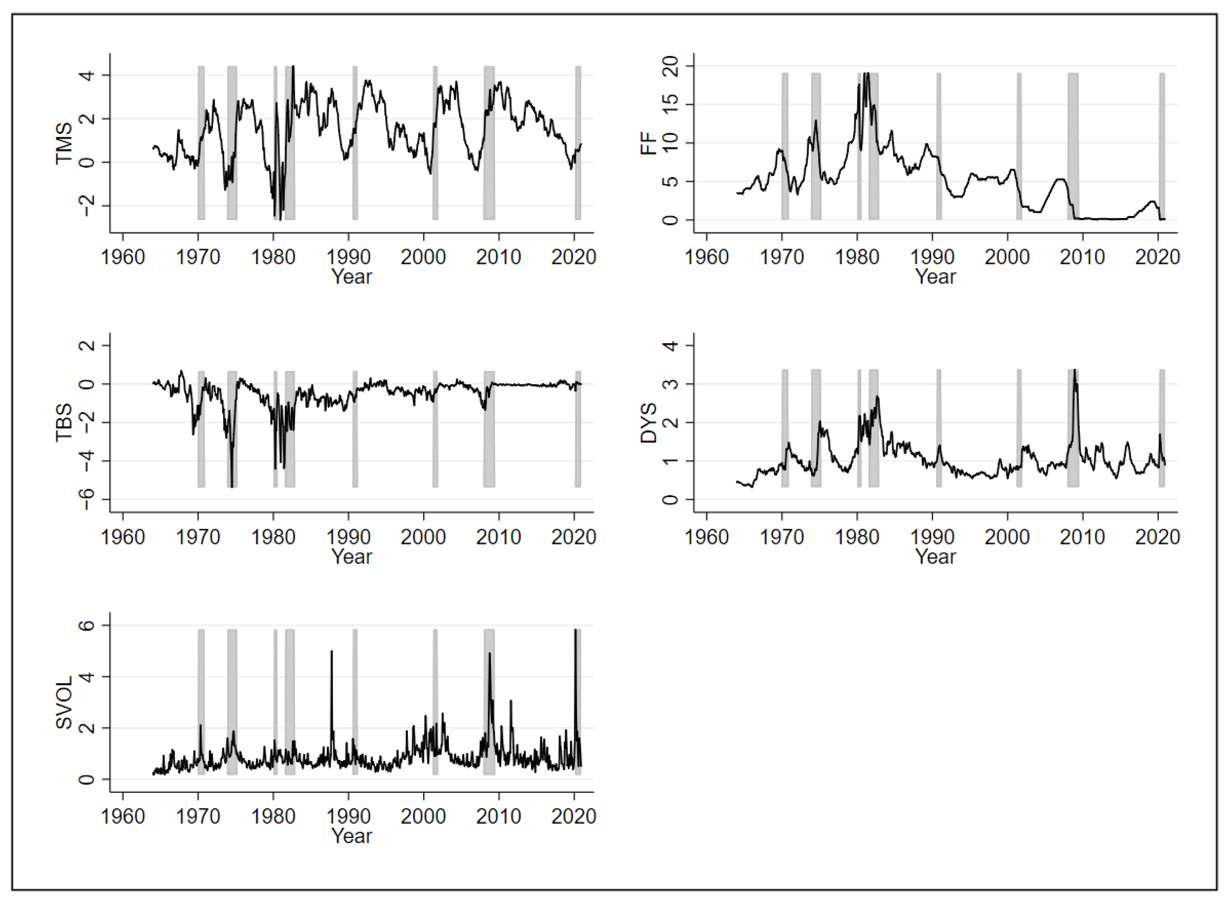
Figure 2 shows the recession probabilities predicted from each model with a forecasting horizon h of 3 months. This plot illustrates that Model 4 makes better predictions of recessions than the other three models. Model 1 performs well at predicting recessions in early 1980s, but not well at forecasting other recessions. Model 2 enhances the predictability of recessions, especially the recessions in the mid 1970s, late 2000s, and early 2020s, while it still does not predict well the recessions in the early 1990s and early 2000s. Moreover, Model 2 generates high probabilities of recessions for the late 1980s, which are not actual recession periods. This false prediction of a recession is due to the high value of $SVOL$ in the late 1980s as noted in Figure 1. Model 3 shows decent forecasting performance by capturing most of the recession periods, although it underestimates the duration of the recession in the 2008–2009 period. Model 4 predicts the 2008–2009 recession better than Model 3 by augmenting Model 3 with additional financial variables, which shows that those financial variables are especially useful in improving the predictability of the recession associated with the financial crisis. Additionally, the recession probabilities predicted from Model 4 for the late 1980s are significantly lower than those from Model 2. We can see that accounting for the temporal dependence in the recession indicator by adding temporal cubic terms into Model 2 decreases the predicted recession probabilities for the late 1980s, which in turn increases the predictive performance.

The effects of the additional financial variables and temporal cubic terms for the recession predictability, which are illustrated in Figure 2, can be summarized as follows. (i) The additional financial variables ($TMS$, $DYS$, and $SVOL$) help to better predict the recessions in the mid 1970s, late 2000s, and early 2020s, although they falsely predict a recession in the late 1980s. They are especially useful in predicting the duration of the 2008–2009 recession. (ii) The temporal cubic terms improve the predictability of most recessions, even though they downplay the duration of the recession associated with the 2007 global financial crisis. In particular, they predict the recessions in the early 1990s and early 2000s better than the financial variables. (iii) The additional financial variables and temporal cubic terms complement each other so that they jointly can forecast most of the recessions fairly precisely. The temporal cubic terms help to correct a false detection of a recession from the additional financial variables, while the additional financial variables help to improve the predictability of the recession in the late 2000s, which is not properly captured by the temporal cubic terms.

To further investigate the performance of recession prediction for the longer forecasting horizon,

Table 5. Probit regression results for forecasting recessions over the next 6 or 12 months. This table reports the recession forecasting regression results of the four empirical models specified in Section 3.2. Panel A is with a forecasting horizon h of 6 months, while Panel B is with a forecasting horizon h of 12 months. Columns (1)–(4) are for Models 1–4 in Section 3.2, respectively. $TMS$ refers to the term spread, $FF$ the federal funds rate, $TBS$ the Treasury bill spread, $DYS$ the default yield spread, $SVOL$ the stock market volatility, $DT$ the number of years passed since the last recession, and AIC the Akaike information criterion. t-statistics are reported in parentheses. *** and ** indicate significance at the 1% and 5% levels, respectively.

Panel A: Forecasting Horizon of 6 Months
	(1)	(2)	(3)	(4)
TMS	−0.221 ***	−0.420 ***	−0.560 ***	−0.465 ***
	(−4.21)	(−5.49)	(−6.26)	(−4.63)
FF	0.105 ***	−0.042	0.053 **	−0.039
	(6.14)	(−1.34)	(2.18)	(−1.06)
TBS		−0.796 ***		−0.827 ***
		(−4.77)		(−4.52)
DYS		1.011 ***		0.2220
		(5.24)		(0.97)
SVOL		0.694 ***		0.586 ***
		(5.02)		(3.84)
DT			−1.617 ***	−1.363 ***
			(−7.69)	(−5.77)
$D{T}^2$			0.267 ***	0.233 ***
			(5.22)	(4.12)
$D{T}^3$			−0.012 ***	−0.011 ***
			(−3.56)	(−2.89)
Constant	−1.200 ***	−2.390 ***	1.127 ***	−0.1460
	(−7.84)	(−9.94)	(3.30)	(−0.32)
Observations	678	678	678	678
Pseudo $R^2$	0.15	0.40	0.44	0.53
Log-likelihood	−277.96	−195.95	−183.87	−154.85
AIC	561.91	403.89	379.75	327.70
Panel B: Forecasting Horizon of 12 Months
	(1)	(2)	(3)	(4)
TMS	−0.423 ***	−1.035 ***	−1.168 ***	−1.555 ***
	(−7.58)	(−9.36)	(−8.83)	(−8.39)
FF	0.150 ***	−0.038	0.130 ***	−0.055
	(7.63)	(−0.97)	(4.47)	(−1.07)
TBS		−1.323 ***		−1.849 ***
		(−5.24)		(−5.82)
DYS		1.702 ***		0.721 **
		(6.82)		(2.48)
SVOL		0.676 ***		0.611 ***
		(4.34)		(2.96)
DT			−1.989 ***	−1.659 ***
			(−7.60)	(−5.34)
$D{T}^2$			0.304 ***	0.223 ***
			(5.07)	(3.16)
$D{T}^3$			−0.012 ***	−0.0070
			(−3.19)	(−1.60)
Constant	−0.957 ***	−2.313 ***	2.420 ***	1.453 **
	(−6.12)	(−8.20)	(5.49)	(2.35)
Observations	672	672	672	672
Pseudo $R^2$	0.28	0.54	0.56	0.69
Log-likelihood	−275.08	−173.19	−168.17	−118.63
AIC	556.17	358.39	348.35	255.25

presents the estimation results of the four empirical models specified in Section 3.2 with forecasting horizons h of 6 and 12 months. The results show the same patterns as in the estimation results with a forecasting horizon h of 3 months. The in-sample fit of Model 4 is better than those of the other three models, confirming the usefulness of the additional financial variables and temporal cubic terms for recession prediction. One thing to note with regards to the estimated coefficients for Model 4 is the significance of the coefficients on $DYS$. The coefficient on $DYS$ is statistically significant with h = 12, but not with h = 3 nor 6. This suggests that the default yield spread helps to predict recessions in the longer term rather than imminent recessions.

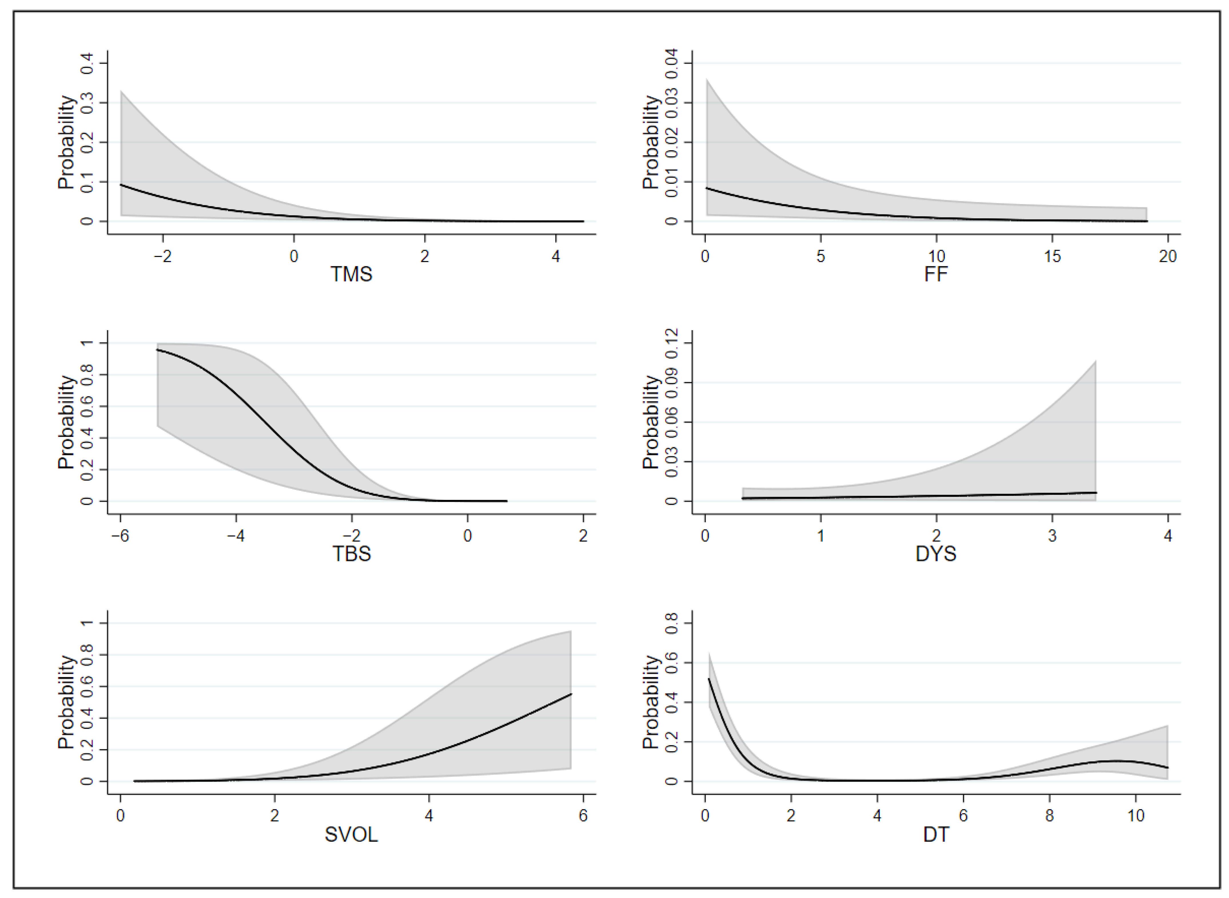
Given that Model 4 has the best in-sample fit among the four empirical models considered, it is interesting to see how each explanatory variable in Model 4 affects the predicted probability of recessions. To this end, Figure 3 plots the predicted probabilities of recessions over a range of values for each explanatory variable, holding all the other explanatory variables at their mean values. All these predicted probabilities are based on Model 4 and horizon h = 3. The following can be noticed from the figure. First, the marginal effects of $TMS$ and $TBS$ show similar patterns: once the value of each variable goes below a certain threshold, the probability of a recession starts to increase as the value of the variable decreases. In particular, the larger size of a negative term spread leads to a higher probability of recessions. Second, $SVOL$ has its own threshold above which the recession probability increases with the value of the variable. The higher the stock market volatility becomes, the higher the recession probability gets. Third, the probability of a recession gradually increases with the value of $DYS$, while it decreases with the value of $FF$. When the default yield spread is larger, the probability for recessions is also higher. Finally, the plot for the marginal effect of $DT$ shows that the recession probability steeply decreases with the value of $DT$ as long as $DT$ is less than about 2 years. However, the probability of a recession starts to slowly increase once $DT$ exceeds around 6 years, which implies that a period of expansions for more than about 6 years starts to bring in a higher probability of recessions.

4.2. Out-of-Sample Forecasting Performance

In this section, I examine the usefulness of the empirical models specified in Section 3.2 for the out-of-sample forecasting of recessions. The in-sample estimation in Section 4.1 assumes that all information for the whole sample period is available at the time when the forecasting is made. However, for those who want to use estimated models for forecasting future recessions, this assumption is not realistic. Out-of-sample forecasting is, therefore, estimated using only the information available at the time of forecasting. Starting with the recession prediction made in December 1979, the predicted recession probability in each month is calculated using only the data available up to the time at which the prediction is made. The root mean squared error (RMSE) for each forecasting horizon h is then computed as follows:

$$RMS{E}_h=\sqrt{{\displaystyle \frac{1}{T_h}}\sum _{t=1}^{T_h}{({\widehat{p}}_{t+1,t+h}-RE{C}_{t+1,t+h})}^2},$$

(8)

where $T_h$ is the total number of out-of-sample predictions made, and ${\widehat{p}}_{t+1,t+h}$ is the predicted probability of a recession over the period between t+1 and t+h, which is estimated using only the data available up to time t. In addition to the RMSE, the average prediction error (APE) for each forecasting horizon h is also calculated with a probability threshold of 0.5 as follows:

$$AP{E}_h={\displaystyle \frac{1}{T_h}}\sum _{t=1}^{T_h}\left|𝟙({\widehat{p}}_{t+1,t+h}>0.5)-RE{C}_{t+1,t+h}\right|,$$

(9)

where $𝟙$ denotes an indicator function for the condition in the parenthesis being true. The APE defined above corresponds to the average rate of the false prediction of future recessions when we regard a recession probability greater than a threshold of 0.5 as an indication of a recession.

Table 6. Out-of-sample forecasting errors. This table reports the out-of-sample forecasting errors of the four empirical models specified in Section 3.2. The out-of-sample forecasting performance of each model is evaluated for each forecasting horizon h, starting with the recession prediction made in December 1979 and using only the data available up to the time at which the prediction is made. The root mean squared errors (RMSE) of Equation (8) are reported in Panel A, while the average prediction errors (APE) of Equation (9) are in Panel B. Columns (1)–(4) are for Models 1–4 in Section 3.2, respectively.

Panel A: Root Mean Squared Errors
Horizon	(1)	(2)	(3)	(4)
3	0.3453	0.2942	0.2885	0.2602
6	0.3577	0.3100	0.3088	0.2842
12	0.3620	0.2980	0.3199	0.2775
Panel B: Average Prediction Errors
Horizon	(1)	(2)	(3)	(4)
3	0.1220	0.1057	0.1179	0.0777
6	0.1362	0.1240	0.1382	0.0988
12	0.1911	0.1382	0.1423	0.1125

reports the out-of-sample RMSE and APE of each model for forecasting horizons h of 3, 6, and 12 months. For all three horizons considered, Model 4 shows the best out-of-sample forecasting performance in terms of both RMSE and APE. With a forecasting horizon h of 3 months, Model 1 has an average prediction error of 12.20%, while Model 4 decreases the prediction error by 4.43%p to 7.77%. If we focus on a forecasting horizon h of 12 months, Model 4 reduces the average prediction error by 7.86%p as compared to that from Model 1. In addition, we can see that the RMSE and APE from Model 4 are smaller than those from Models 2 and 3, which indicates that both the additional financial variables and temporal cubic terms help to improve the out-of-sample recession prediction.

Another way of evaluating the out-of-sample forecasting performance is to use a receiver operating characteristic (ROC) curve, which shows the relation between false positive rate (FPR) and true positive rate (TPR). FPR is the ratio between the number of false positive predictions and the number of real negative cases, while TPR is the ratio between the number of true positive predictions and the number of real positive cases. Unlike the APE in Equation (9) which assumes a fixed recession probability threshold of 0.5, the ROC curve is generated by assuming many different values of the recession probability threshold. 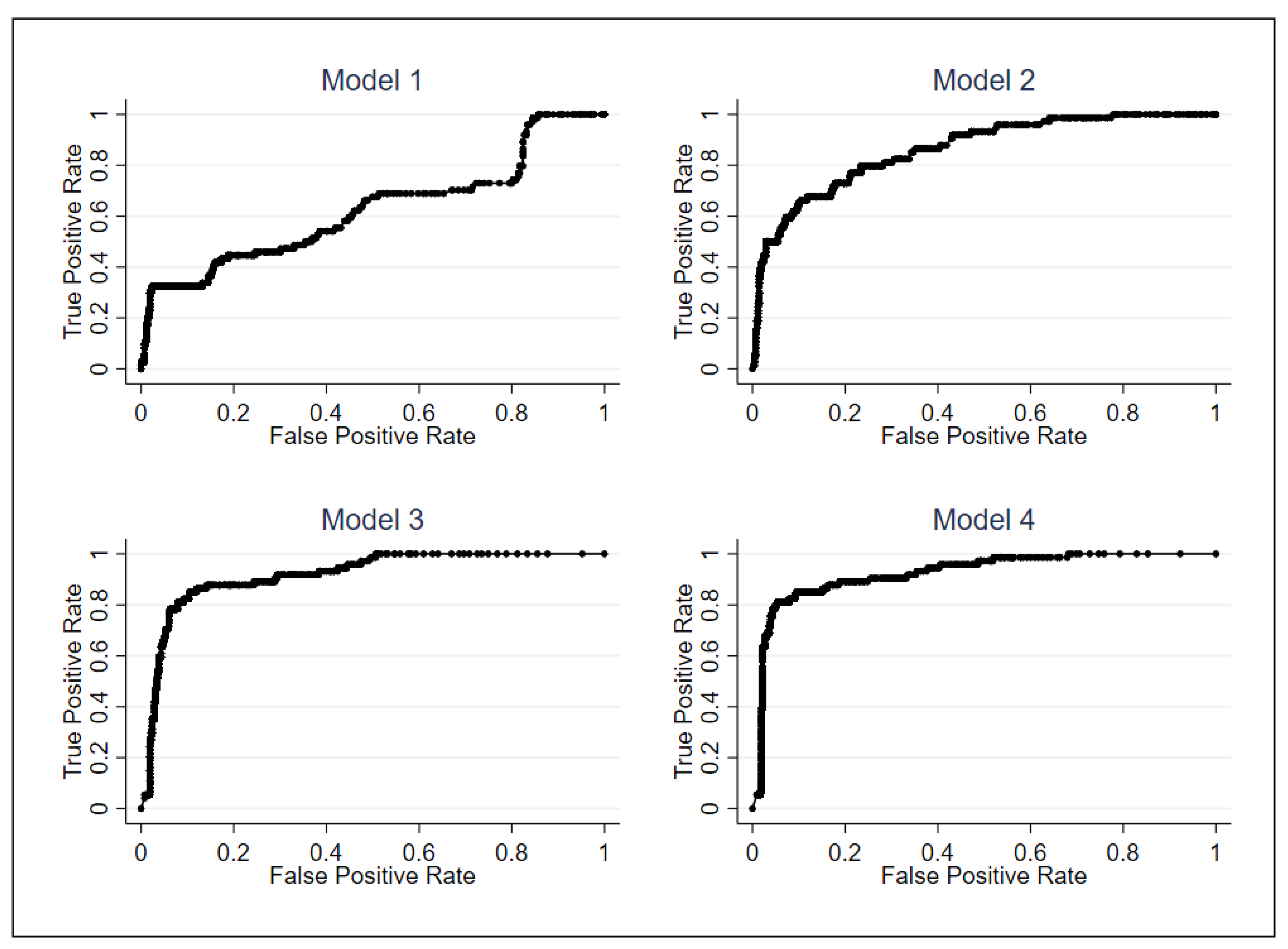Figure 4 shows the ROC curves of the out-of-sample forecasting from the four empirical models specified in Section 3.2 with a forecasting horizon h of 3 months. Each dot in the plot corresponds to a pair of FPR and TPR for a certain value of the recession probability threshold. The out-of-sample forecasting performance of each model can be measured by the area under the curve (AUC) for the ROC curve from each model. The higher value of the AUC implies better forecasting performance. The AUC for each of the Models 1–4 is 0.6247, 0.8624, 0.9179, and 0.9248, respectively, which also confirms that Model 4 has the best out-of-sample forecasting performance among the four models considered.

5. Conclusions

Using U.S. recession data between 1964 and 2020, I show that both additional financial variables, the Treasury bill spread, default yield spread, stock market volatility, and temporal cubic terms help to improve in-sample recession prediction as well as out-of-sample recession prediction. This suggests that the recession forecasting performance of the traditional models can be enhanced by additionally considering relevant financial variables and time dependence. The additional financial variables especially help to improve predictability of recessions associated with financial crises, reflecting the relation between stock market volatility and financial crises noted by Schwert (1989a). The temporal cubic terms also properly capture the temporal dependence structure of a binary recession indicator, consistent with Carter and Signorino (2010). Overall, this study contributes to the literature by documenting the usefulness of additional financial variables and temporal cubic terms for better recession predictability.

These results are not only of practical relevance for recession forecasting, but also are important in enhancing our understanding of business cycles and economic growth more broadly. However, the results in this study are based on U.S. data. The applicability of the variables considered in this study in other countries could, therefore, present potential future research directions. Depending on the characteristics of the nation’s economy, other types of variables could also be considered.

References

1. Akaike, Hirotugu. 1974. A new look at the statistical model identification. IEEE Transactions on Automatic Control 19: 716–23. [Google Scholar] [CrossRef]
2. Ang, Andrew, Monika Piazzesi, and Min Wei. 2006. What does the yield curve tell us about gdp growth? Journal of Econometrics 131: 359–403. [Google Scholar] [CrossRef] [Green Version]
3. Atkinson, Tyler, David Luttrell, and Harvey Rosenblum. 2013. How Bad was It? The Costs and Consequences of the 2007–2009 Financial Crisis. Federal Reserve Bank of Dallas Staff Papers 20: 1–22. [Google Scholar]
4. Bauer, Michael D., and Thomas M. Mertens. 2018. Information in the yield curve about future recessions. FRBSF Economic Letter 20: 1–5. [Google Scholar]
5. Beck, Nathaniel, Jonathan N. Katz, and Richard Tucker. 1998. Taking time seriously: Time-series-cross-section analysis with a binary dependent variable. American Journal of Political Science 42: 1260–88. [Google Scholar] [CrossRef]
6. Benzoni, Luca, Olena Chyruk, and David Kelley. 2018. Why does the yield-curve slope predict recessions? Federal Reserve Bank of Chicago Working Paper 15: 1–17. [Google Scholar]
7. Carter, David B., and Curtis S. Signorino. 2010. Back to the future: Modeling time dependence in binary data. Political Analysis 18: 271–92. [Google Scholar] [CrossRef]
8. Chen, Nai-Fu. 1991. Financial investment opportunities and the macroeconomy. The Journal of Finance 46: 529–54. [Google Scholar] [CrossRef]
9. Choudhry, Taufiq, Fotios I. Papadimitriou, and Sarosh Shabi. 2016. Stock market volatility and business cycle: Evidence from linear and nonlinear causality tests. Journal of Banking & Finance 66: 89–101. [Google Scholar]
10. Corradi, Valentina, Walter Distaso, and Antonio Mele. 2013. Macroeconomic determinants of stock volatility and volatility premiums. Journal of Monetary Economics 60: 203–20. [Google Scholar] [CrossRef]
11. de Lint, Christel Rendu, and David Stolin. 2003. The predictive power of the yield curve: A theoretical assessment. Journal of Monetary Economics 50: 1603–22. [Google Scholar] [CrossRef]
12. Estrella, Arturo. 2005. Why Does the Yield Curve Predict Output and Inflation? The Economic Journal 115: 722–44. [Google Scholar] [CrossRef]
13. Estrella, Arturo, and Gikas A. Hardouvelis. 1991. The term structure as a predictor of real economic activity. The Journal of Finance 46: 555–76. [Google Scholar] [CrossRef]
14. Estrella, Arturo, and Frederic S. Mishkin. 1997. The predictive power of the term structure of interest rates in europe and the united states: Implications for the european central bank. European Economic Review 41: 1375–401. [Google Scholar] [CrossRef]
15. Estrella, Arturo, and Frederic S. Mishkin. 1998. Predicting us recessions: Financial variables as leading indicators. Review of Economics and Statistics 80: 45–61. [Google Scholar] [CrossRef]
16. Estrella, Arturo, Anthony P. Rodrigues, and Sebastian Schich. 2003. How stable is the predictive power of the yield curve? evidence from germany and the united states. Review of Economics and Statistics 85: 629–44. [Google Scholar] [CrossRef] [Green Version]
17. Fama, Eugene F. 1986. Term premiums and default premiums in money markets. Journal of Financial Economics 17: 175–96. [Google Scholar] [CrossRef] [Green Version]
18. Fama, Eugene F. 1990. Stock returns, expected returns, and real activity. The Journal of Finance 45: 1089–108. [Google Scholar] [CrossRef]
19. Fama, Eugene F., and Robert R. Bliss. 1987. The information in long-maturity forward rates. The American Economic Review 77: 680–92. [Google Scholar]
20. Fama, Eugene F., and Kenneth R. French. 1989. Business conditions and expected returns on stocks and bonds. Journal of Financial Economics 25: 23–49. [Google Scholar] [CrossRef]
21. Fama, Eugene F., and Kenneth R. French. 1993. Common risk factors in the returns on stocks and bonds. Journal of Financial Economics 33: 3–56. [Google Scholar] [CrossRef]
22. Fama, Eugene F., and Kenneth R. French. 2015. A five-factor asset pricing model. Journal of Financial Economics 116: 1–22. [Google Scholar] [CrossRef] [Green Version]
23. Fendel, Ralf, Nicola Mai, and Oliver Mohr. 2021. Recession probabilities for the eurozone at the zero lower bound: Challenges to the term spread and rise of alternatives. Journal of Forecasting 40: 1000–26. [Google Scholar] [CrossRef]
24. Gilchrist, Simon, and Egon Zakrajšek. 2012. Credit spreads and business cycle fluctuations. American Economic Review 102: 1692–720. [Google Scholar] [CrossRef]
25. Hamilton, James D., and Gang Lin. 1996. Stock market volatility and the business cycle. Journal of Applied Econometrics 11: 573–93. [Google Scholar] [CrossRef]
26. King, Robert G., Charles I. Plosser, and Sergio T. Rebelo. 1988. Production, growth and business cycles: I. the basic neoclassical model. Journal of Monetary Economics 21: 195–232. [Google Scholar] [CrossRef]
27. Kydland, Finn E., and Edward C. Prescott. 1982. Time to build and aggregate fluctuations. Econometrica 50: 1345–70. [Google Scholar] [CrossRef]
28. Long, John B., and Charles I. Plosser. 1983. Real business cycles. Journal of Political Economy 91: 39–69. [Google Scholar] [CrossRef]
29. Lucas, Robert E. 1977. Understanding business cycles. Carnegie-Rochester Conference Series on Public Policy 5: 7–29. [Google Scholar] [CrossRef]
30. Plosser, Charles I. 1989. Understanding real business cycles. Journal of Economic Perspectives 3: 51–77. [Google Scholar] [CrossRef]
31. Schwert, G. William. 1989a. Business cycles, financial crises, and stock volatility. Carnegie-Rochester Conference Series on Public Policy 31: 83–125. [Google Scholar] [CrossRef] [Green Version]
32. Schwert, G. William. 1989b. Why does stock market volatility change over time? The Journal of Finance 44: 1115–53. [Google Scholar] [CrossRef]
33. Schwert, G. William. 1990. Stock returns and real activity: A century of evidence. The Journal of Finance 45: 1237–57. [Google Scholar] [CrossRef]
34. Wright, Jonathan H. 2006. The Yield Curve and Predicting Recessions. FEDS Working Paper 7: 1–19. [Google Scholar]
Figure 1. Time series of financial variables. This figure shows the time series of the financial variables over the period between 1964 and 2020. T M S refers to the term spread, F F the federal funds rate, T B S the Treasury bill spread, D Y S the default yield spread, and S V O L the stock market volatility. All the financial variables are denominated in percentage (%) terms. The shaded areas correspond to the U.S. recession periods.
Economies 09 00118 g001
Figure 2. Predicted recession probability. This figure shows the recession probabilities predicted from the in-sample estimation of the four empirical models specified in Section 3.2 with a forecasting horizon h of 3 months. The shaded areas in the figure refer to the periods in which there was a recession over the next three months.
Economies 09 00118 g002
Figure 3. Marginal effects on recession probability. This figure shows the predicted recession probabilities over a range of values for each explanatory variable, holding all the other explanatory variables at their mean values. The predicted probabilities are based on Model 4 and horizon h = 3. T M S refers to the term spread, F F the federal funds rate, T B S the Treasury bill spread, D Y S the default yield spread, S V O L the stock market volatility, and D T the number of years passed since the last recession. The shaded bands correspond to 95% confidence intervals.
Economies 09 00118 g003
Figure 4. Receiver operating characteristic (ROC) curves. This figure shows the receiver operating characteristic (ROC) curves of the out-of-sample forecasting from the four empirical models specified in Section 3.2 with a forecasting horizon h of 3 months.
Economies 09 00118 g004