The Cost of Overcoming the Zero Lower-Bound: A Welfare Analysis †


Abstract
1. Introduction
2. Breaking through the Lower-Bound
2.1. Cash Abolition
2.2. Negative Interest Rates on Cash
2.2.1. Depreciative Money (Schwundgeld)
2.2.2. The Flexible Exchange Rate between Cash and Bank Deposits
2.2.3. Taxes on Cash
3. Welfare Losses Due to Negative Interest Rates on Cash
3.1. Sidrauski Model with Interest Rates on Cash
3.2. Quantification of the Welfare Losses of Negative Interest Rates on Cash Holdings
3.3. Sensitivity Analysis
4. Negative Interest Rates on Broader Monetary Aggregates
5. Summary and Conclusions
Author Contributions
Funding
Acknowledgments
Conflicts of Interest
Appendix A. Sidrauski Model with CRRA Utility Function
Appendix B. Data Basis

| Period | 2005 | 2015 | ||||
|---|---|---|---|---|---|---|
| EMU | GY | EMU | GY | |||
| Private Consumption | C | € bn. | 4765 | 1329 | 5743 | 1636 |
| Gross Domestic Product | GDP | € bn. | 8460 | 2301 | 10,460 | 3033 |
| Monetary Aggregates | ||||||
| Cash in circulation | M0 | € bn. | 533 | 143 | 1049 | 244 |
| plus overnight deposits | M1 | € bn. | 3480 | 869 | 6631 | 2010 |
| plus term and savings deposits | M3 | € bn. | 7117 | 1737 | 10,833 | 2897 |
| Average growth rates | ||||||
| Private Consumption | C | % | 1.9 | 2.1 | ||
| Gross Domestic Product | GDP | % | 2.1 | 2.8 | ||
| Cash in circulation | M0 | % | 7.0 | 5.5 | ||
| plus overnight deposits | M1 | % | 6.7 | 8.7 | ||
| plus term and savings deposits | M3 | % | 4.3 | 5.2 | ||
| Interest rates | ||||||
| Government bond yield *) | % | 3.4 | 3.4 | 1.2 | 0.6 | |
| Real return on financial wealth **) | % | 4.0 | 2.6 | |||
| Nominal return of financial wealth +) | z | % | 6.1 | 6.0 | 4.2 | 3.5 |
| Opportunity costs of overnight deposits | z-s2 | % | 5.4 | 4.8 | 4.0 | 3.4 |
| Opportunity costs of term deposits ++) | z-s3 | % | 3.9 | 3.5 | 3.5 | 2.8 |
| User costs of money | ||||||
| Cash in circulation | k1 | € bn. | 32 | 9 | 44 | 9 |
| plus overnight deposits | k2 | € bn. | 190 | 44 | 267 | 68 |
| plus term and savings deposits | k3 | € bn. | 333 | 74 | 413 | 93 |
| Preference parameters | ||||||
| Cash in circulation | α1 | % | 0.64 | 0.62 | 0.71 | 0.50 |
| Overnight deposits | α2 | % | 3.10 | 2.50 | 3.63 | 3.44 |
| Term and savings deposits | α3 | % | 2.79 | 2.17 | 2.36 | 1.43 |
| Sum | W | % | 6.53 | 5.28 | 6.70 | 5.37 |
References
- Adams, John. 2006. The War on Cash. European Card Review March/April: 12–18. [Google Scholar]
- Agarwal, Ruchir, and Miles Kimball. 2015. Breaking Through the Zero Lower-Bound. IMF Working Paper WP/15/224. Washington, DC, USA: International Monetary Fund. [Google Scholar]
- Agarwal, Ruchir, and Miles Kimball. 2019. Enabling Deep Negative Rates to Fight Recessions: A Guide. IMF Working Paper WP/19/84. Washington, DC, USA: International Monetary Fund. [Google Scholar]
- Bagnall, John, David Bounie, Kim P. Huynh, Anneke Kosse, Tobias Schmidt, Scott Schuh, and Helmut Stix. 2016. Consumer Cash Usage: A Cross-Country Comparison with Payment Diary Survey Data. International Journal of Central Banking 12: 1–61. [Google Scholar] [CrossRef][Green Version]
- Bank for International Settlements (BIS). 2015. Annual Report 2015, April. Basel: Bank for International Settlements (BIS). [Google Scholar]
- Bartzsch, Nikolaus, Gerhard Rösl, and Franz Seitz. 2013. Currency Movements Within and Outside a Currency Union: The case of Germany and the euro area. Quarterly Review of Economics and Finance 53: 393–401. [Google Scholar] [CrossRef][Green Version]
- Bech, Morten L., and Aytek Malkhozov. 2016. How have Central Banks Implemented Negative Policy Rates? BIS Quarterly Review March: 31–44. [Google Scholar]
- Blanchard, Oliver J., and Stanley Fischer. 1989. Lectures on Macroeconomics. Cambridge: MIT Press. [Google Scholar]
- Buiter, Willem M. 2009. Negative Nominal Interest Rates: Three Ways to Overcome the Zero Lower-bound. The North American Journal of Economics and Finance 20: 213–38. [Google Scholar] [CrossRef]
- Buiter, Willem, and Ebrahim Rahbari. 2015. High Time to Get Low: Getting Rid of the Lower-bound on Nominal Interest Rates. Global Economics View, Citi Research, April 9. [Google Scholar]
- Bundesbank, Deutsche. 2015. German Households’ Saving and Investment Behavior in Light of the Low-interest-rate Environment. Monthly Report 10: 13–31. [Google Scholar]
- Bundesbank, Deutsche. 2016. The Macroeconomic Impact of Quantitative Easing in the Euro Area. Monthly Report 6: 29–53. [Google Scholar]
- Corsetti, Giancarlo, Eleonora Mavroeidi, Gregory Thwaites, and Martin Wolf. 2019. Step Away from the Zero Lower-bound: Small open economies in a world of secular stagnation. Journal of International Economics 116: 88–102. [Google Scholar] [CrossRef]
- Croushore, Dean. 1993. Money in the Utility Function: A Functional Equivalence to a Shopping-time Model. Journal of Macroeconomics 15: 175–82. [Google Scholar] [CrossRef]
- Esselink, Henk, and Lola Hernández. 2017. The Use of Cash by Households in the Euro Area. ECB Occasional Paper Series No 201; Amsterdam: Elsevier. [Google Scholar]
- EU-Commission. 2010. Commission Adopts a Recommendation on the Scope and Effects of Legal Tender of Euro Banknotes and Coins. Press Release of 22 March 2010. Brussels: EU-Commission. [Google Scholar]
- EU-Commission. 2017. Proposal for an EU Initiative on Restrictions on Payments in Cash, 23.1.2017. Brussels: EU-Commission. [Google Scholar]
- Feenstra, Robert C. 1986. Functional Equivalence between Liquidity Costs and the Utility of Money. Journal of Monetary Economics 17: 271–91. [Google Scholar] [CrossRef]
- Fisher, Irving. 1933. Stamp Scrip. New York: Adelphi Company Publishers. [Google Scholar]
- Friedman, Milton. 1969. The Optimum Quantity of Money and Other Essays. London: Aldine Transaction. [Google Scholar]
- Gesell, Silvio. 1911. Die neue Lehre vom Geld. Berlin: Physiokratischer-Verlag. [Google Scholar]
- Gesell, Silvio. 1949. Die natürliche Wirtschaftsordnung durch Freiland und Freigeld. Lauf bei Nürnberg: Rudolf Zitzmann Publisher. [Google Scholar]
- Harper, Joel W. 1948. Scrip and Other Forms of Local Money. Ph.D. dissertation, University of Chicago, Chicago, IL, USA. [Google Scholar]
- Havranek, Tomas, Roman Horvath, Zuzana Irsova, and Marek Rusnak. 2015. Cross-Country Heterogeneity in Intertemporal Substitution. Journal of International Economics 96: 100–18. [Google Scholar] [CrossRef]
- Holman, Jill A. 1998. GMM Estimation of a Money-in-the-Utility-Function Model: The Implications of Functional Forms. Journal of Money Credit and Banking 30: 679–98. [Google Scholar] [CrossRef]
- Johansson, Per-Olov. 1991. An Introduction to Modern Welfare Economics. Cambridge: Cambridge University Press. [Google Scholar]
- Keynes, John M. 1936. The General Theory of Employment, Interest and Money. London: Palgrave Macmillan. [Google Scholar]
- Krüger, Malte, and Franz Seitz. 2017. Costs and Benefits of Cash and Cashless Payment Instruments (Module 2): The Benefits of Cash. Frankfurt: Fritz Knapp Publisher. [Google Scholar]
- Lucas, Robert E., Jr. 2000. Inflation and Welfare. Econometrica 68: 247–74. [Google Scholar] [CrossRef]
- Michail, Nektarios. 2018. What if they had not Gone Negative? A counterfactual assessment of the impact from negative interest rates. Oxford Bulletin of Economics & Statistics 81: 1–19. [Google Scholar]
- Miracle of Wörgl. 1932. Available online: https://en.wikipedia.org/wiki/W%C3%B6rgl#The_W%C3%B6rgl_Experiment (accessed on 5 March 2019).
- Papadamou, Stephanos, Nikolaos A. Kyriazis, and Panayiotis G. Tzeremes. 2019. Unconventional Monetary Policy Effects on Output and Inflation: A meta-analysis. International Review of Financial Analysis 61: 295–305. [Google Scholar] [CrossRef]
- Priftis, Romanos, and Lukas Vogel. 2017. The Macroeconomic Effects of the ECB’s Evolving QE Programme: A model-based analysis. Open Econ Review 28: 823–45. [Google Scholar] [CrossRef]
- Rogoff, Kenneth S. 2016. The Curse of Cash. Princeton and Oxford: Princeton University Press. [Google Scholar]
- Romer, David. 2019. Advanced Macroeconomics, 5th ed.Boston: McGraw-Hill. [Google Scholar]
- Rösl, Gerhard. 2006. Regional Currencies in Germany—Local Competition for the Euro? Discussion Paper, Series 1, No 43/2006; Frankfurt: Deutsche Bundesbank. [Google Scholar]
- Rösl, Gerhard, and Karl-Heinz Tödter. 2015. The Costs and Welfare Effects of ECB’s Financial Repression Policy: Consequences for German Savers. Review of Economics and Finance 5: 42–59. [Google Scholar]
- Rösl, Gerhard, Franz Seitz, and Karl-Heinz Tödter. 2017. Doing Away with Cash? The Welfare costs of Abolishing Cash. Working Paper No. 112. Frankfurt, Germany: Institute for Monetary and Financial Stability (IMFS). [Google Scholar]
- Sands, Peter. 2016. Making it Harder for the Bad Guys: The Case for Eliminating High Denomination Notes. m-rcbg Associate Working Paper Series No. 52; Cambridge: Harvard Kennedy School. [Google Scholar]
- Sidrauski, Miguel. 1967. Rational Choice and Patterns of Growth in a Monetary Economy. American Economic Review LVII: 534–44. [Google Scholar]
- Timberlake, Richard H. 1987. Private Production of Scrip-Money in the Isolated Community. Journal of Money Credit and Banking 19: 437–47. [Google Scholar] [CrossRef]
- Van Hove, Leo. 2016. Could “Nudges” Steer us towards a Less-Cash Society? In Transforming Payment Systems in Europe. Edited by J. Górka. Basingstoke: Palgrave Macmillan, pp. 70–110. [Google Scholar]
- Wakamori, N., and A. Welte. 2017. Why Do Shoppers Use Cash? Evidence from Shopping Diary Data. Journal of Money Credit and Banking 49: 115–69. [Google Scholar] [CrossRef]
- Walsh, Carl E. 2017. Monetary Theory and Policy, 4th ed. Cambridge: The MIT Press. [Google Scholar]
- Warner, Jonathan. 2014. The Future of Community Currencies: Physical cash or solely electronic? Paper presented at International Cash Conference on the Usage Costs and Benefits of Cash Revisited 2014, Dresden, Germany, September 16–18. [Google Scholar]
- Witmer, Jonathan, and Jing Yang. 2016. Estimating Canada’s Effective Lower-Bound. Bank of Canada Review. Ottawa: Bank of Canada, pp. 3–14. [Google Scholar]
| 1 | A more traditional case against cash is that it would help to fight corruption, tax evasion, drug trade, and terrorist financing (Rogoff 2016; Sands 2016). See Krüger and Seitz (2017, chp. 7.1) for a critical assessment. On the motivation of cash usage from a shopper’s perspective see Wakamori and Welte (2017). |
| 2 | For example, the “Miracle of Wörgl”, (Miracle of Wörgl 1932), was started during the Great Depression on 31 July 1932 with the issuing of ‘Certified Compensation Bills’, a form of local “Schwundgeld”. This was an application of the monetary theories of Silvio Gesell by the town’s then-mayor Michael Unterguggenberger. The experiment increased local employment and several local government projects could be completed, seeming to defy the depression in the country. Despite attracting great interest at the time, including the French Premier Edouard Daladier and Irving Fisher, the experiment was terminated by the Austrian central bank on 1 September 1933. |
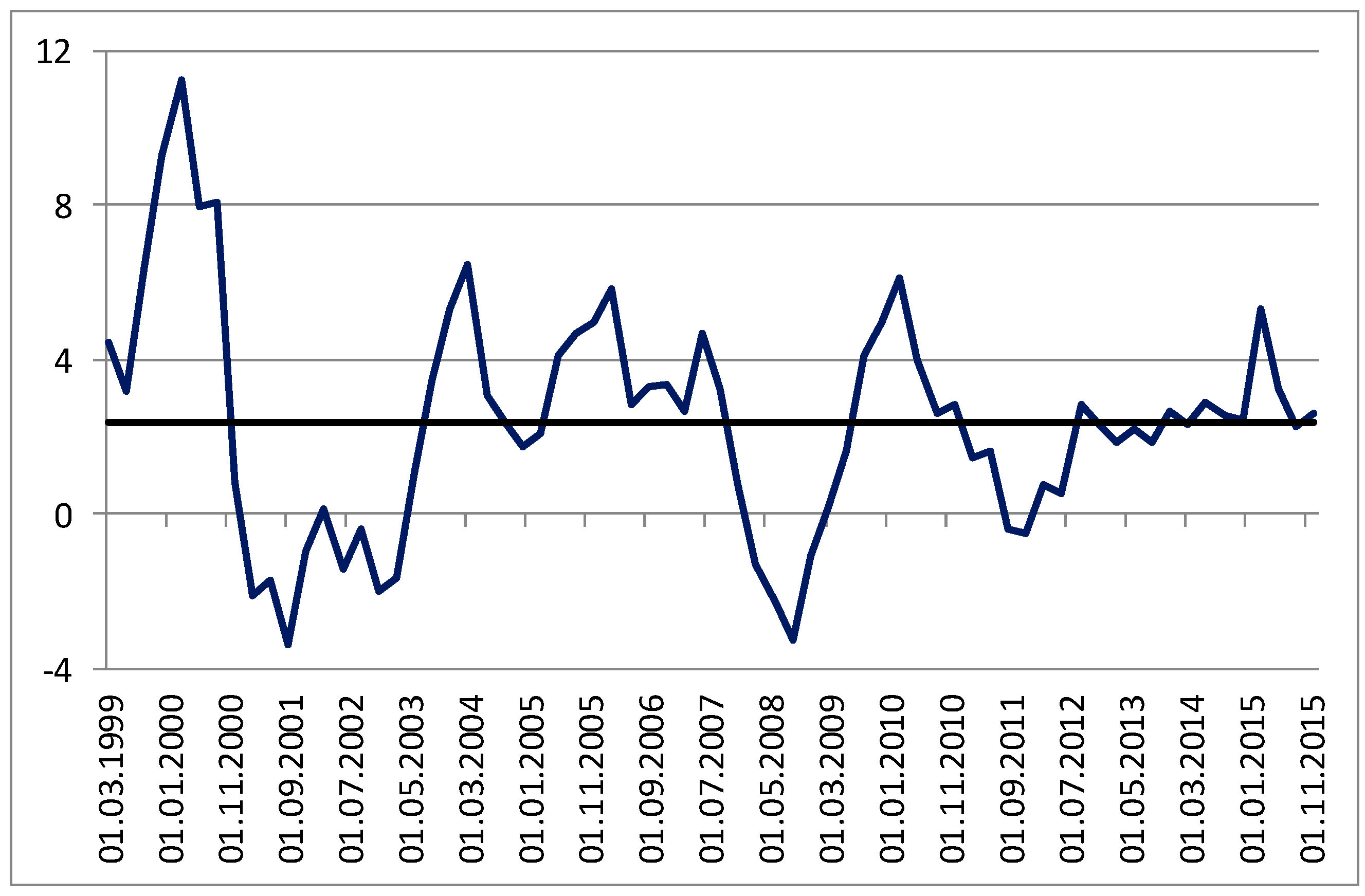
| 3 | |
| 4 | Agarwal and Kimball (2015) speak of a crawling peg. If this exchange rate would be a free market rate it is not clear beforehand whether it would settle eventually above or below par. |
| 5 | In this section money only consists of cash. However, Section 5 considers broader monetary aggregates. |
| 6 | On “money in the utility function” (MIU) models, see Sidrauski (1967), Walsh (2017, chp. 2). Feenstra (1986) proves that a cash-in-advance approach is a special case of MIU, while Croushore (1993) shows that MIU and shopping-time-models are equivalent. Holman (1998) succeeds in incorporating transaction, precautionary, and store-of-value motives in a MIU model. |
| 7 | This corresponds to the recycling of seigniorage from cash issuance (including transfer of real resources to the money producers owing to negative interest rates on nominal money holdings). |
| 8 | To keep things simple, the (capital market) interest rate r is assumed exogenous, although an endogenous interest rate (by introducing a production function) would not substantially alter the model results. For similar reasons, depreciation of the capital stock is not taken into consideration either. |
| 9 | |
| 10 | Whether or not such considerations are also appropriate for actions taken by a democratically non-legitimized central bank as the ECB is an open question, see Rösl and Tödter (2015, p. 43). |
| 11 | If the money demand function is linear, the excess burden is equivalent to the so called “Harberger triangle”. |
| 12 | For a more detailed treatment see Rösl et al. (2017). |
| 13 | In 2017, the real yield was only at 1.4%. |
| 14 | This leads to a small underestimation of the opportunity costs of the corresponding monetary asset, as interest rates on savings deposits are lower. The same holds for overnight deposits. |


| Interest Rate on Cash | s | Unit | 0 | −0.01 | −0.02 | −0.03 | −0.04 | −0.05 | −0.10 |
|---|---|---|---|---|---|---|---|---|---|
| Euro Area | |||||||||
| User cost of cash | z | rate | 0.04 | 0.05 | 0.06 | 0.07 | 0.08 | 0.09 | 0.14 |
| Cash demand | M0 | € bn. | 1049 | 846 | 708 | 609 | 535 | 476 | 308 |
| Velocity of circulaton *) | υ~ | 1.0 | 1.2 | 1.5 | 1.7 | 2.0 | 2.2 | 3.4 | |
| Loss in consumer surplus | CS | € bn. | 0 | 9.4 | 17.1 | 23.7 | 29.4 | 34.4 | 53.4 |
| Additional gov. revenues | SE | € bn. | 0 | 8.5 | 14.2 | 18.3 | 21.4 | 23.8 | 30.8 |
| Deadweight loss | DWL | € bn. | 0 | 0.9 | 3.0 | 5.4 | 8.0 | 10.6 | 22.6 |
| Compensating cons. level | C_X | € bn. | 5743 | 5752 | 5760 | 5767 | 5772 | 5777 | 5796 |
| Equivalent variation | EV | € bn. | 0 | −9.3 | −17.0 | −23.5 | −29.1 | −34.1 | −52.8 |
| Compensating variation | CV | € bn. | 0 | −9.3 | −17.0 | −23.6 | −29.2 | −34.3 | −53.3 |
| per capita | cvp | € | 0 | −28 | −1 | −70 | −87 | −102 | −158 |
| as a share in cons. | cvc | % | 0 | −0.16 | −0.30 | −0.41 | −0.51 | −0.60 | −0.93 |
| as a share in GDP | cvb | % | 0 | −0.09 | −0.16 | −0.23 | −0.28 | −0.33 | −0.51 |
| Germany | |||||||||
| User costs of cash | z | rate | 0.04 | 0.05 | 0.06 | 0.07 | 0.08 | 0.09 | 0.14 |
| Cash demand | M0 | € bn. | 244 | 190 | 156 | 132 | 114 | 101 | 64 |
| Velocity of circulation *) | υ~ | 1.0 | 1.3 | 1.6 | 1.9 | 2.1 | 2.4 | 3.8 | |
| Loss in consumer surplus | CS | € bn. | 0 | 2.1 | 3.9 | 5.3 | 6.5 | 7.6 | 11.6 |
| Add. gov. revenues | SE | € bn. | 0 | 1.9 | 3.1 | 4.0 | 4.6 | 5.1 | 6.4 |
| Deadweight loss | DWL | € bn. | 0 | 0.2 | 0.8 | 1.3 | 2.0 | 2.6 | 5.2 |
| Compensating cons. level | C_X | € bn. | 1636 | 1638 | 1640 | 1641 | 1642 | 1644 | 1648 |
| Equivalent variation | EV | € bn. | 0 | −2.1 | −3.8 | −5.3 | −6.5 | −7.5 | −11.5 |
| Compensating variation | CV | € bn. | 0 | −2.1 | −3.9 | −5.3 | −6.5 | −7.6 | −11.6 |
| per capita | cvp | € | 0 | −26 | −47 | −64 | −79 | −92 | −141 |
| as a share in cons. | cvc | % | 0 | −0.13 | −0.24 | −0.32 | −0.40 | −0.46 | −0.71 |
| as a share in GDP | cvb | % | 0 | −0.07 | −0.13 | −0.17 | −0.21 | −0.25 | −0.38 |
| CV | cvc | cvb | ||||
|---|---|---|---|---|---|---|
| Change of … | € bn. | % | % | |||
| 0.50 | −14 | −0.24 | −0.13 | |||
| Elasticity of substitution | σ | 1.00 | −24 | −0.41 | −0.23 | |
| 2.00 | −36 | −0.63 | −0.35 | |||
| 0.50 | −16 | −0.27 | −0.15 | |||
| Preference parameter | α | % | 0.75 | −24 | −0.41 | −0.23 |
| 1.00 | −31 | −0.54 | −0.30 | |||
| 6.00 | −18 | −0.31 | −0.17 | |||
| Nominal yield of financial wealth | z | % | 4.16 | −24 | −0.41 | −0.23 |
| 2.00 | −40 | −0.69 | −0.38 |
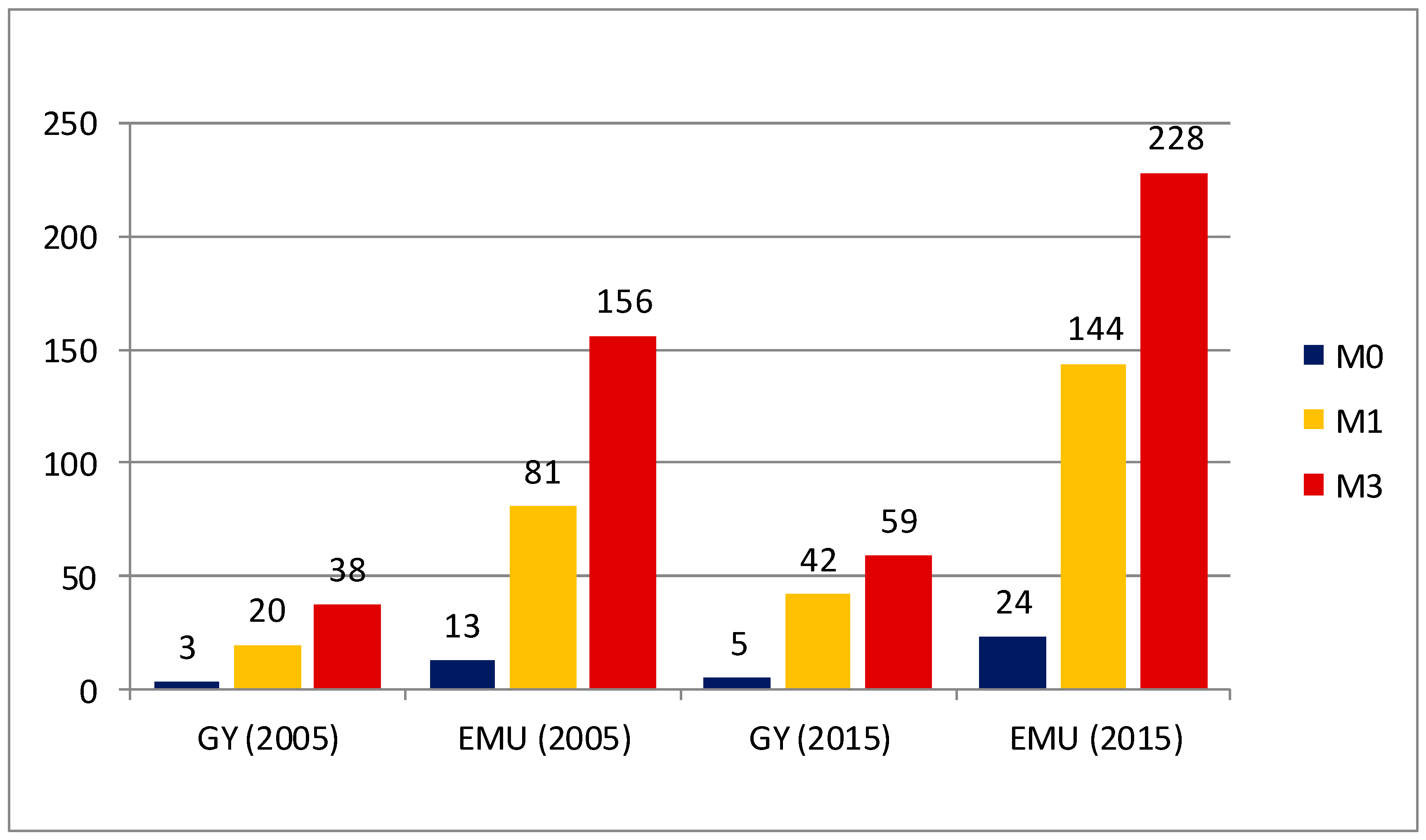
| 2005 | 2015 | |||||
|---|---|---|---|---|---|---|
| EMU | GY | EMU | GY | |||
| Cash M0 | ||||||
| Compensating Variation | CV | € bn. | −13 | −3 | −24 | −5 |
| share in GDP | cvb | % | −0.15 | −0.15 | −0.23 | −0.17 |
| Monetary aggregate M1 | ||||||
| Compensating variation | CV | € bn. | −81 | −20 | −144 | −42 |
| share in GDP | cvb | % | −0.95 | −0.87 | −1.38 | −1.38 |
| Monetary aggregate M3 | ||||||
| Deadweight loss | DWL *) | € bn. | 50 | 14 | 62 | 18 |
| per capita | € | 149 | 169 | 183 | 213 | |
| share in GDP | % | 0.59 | 0.60 | 0.59 | 0.58 | |
| Compensating consumption | C_X | € bn. | 4921 | 1366 | 5971 | 1695 |
| Compensating variation | CV | −156 | −38 | −228 | −59 | |
| per capita | cvp | € | −463 | −460 | −676 | −720 |
| share in consumption | cvc | % | −3.27 | −2.84 | −3.97 | −3.61 |
| share in GDP | cvb | % | −1.84 | −1.64 | −2.18 | −1.95 |
© 2019 by the authors. Licensee MDPI, Basel, Switzerland. This article is an open access article distributed under the terms and conditions of the Creative Commons Attribution (CC BY) license (http://creativecommons.org/licenses/by/4.0/).
Share and Cite
Rösl, G.; Seitz, F.; Tödter, K.-H. The Cost of Overcoming the Zero Lower-Bound: A Welfare Analysis. Economies 2019, 7, 67. https://doi.org/10.3390/economies7030067
Rösl G, Seitz F, Tödter K-H. The Cost of Overcoming the Zero Lower-Bound: A Welfare Analysis. Economies. 2019; 7(3):67. https://doi.org/10.3390/economies7030067
Chicago/Turabian StyleRösl, Gerhard, Franz Seitz, and Karl-Heinz Tödter. 2019. "The Cost of Overcoming the Zero Lower-Bound: A Welfare Analysis" Economies 7, no. 3: 67. https://doi.org/10.3390/economies7030067
APA StyleRösl, G., Seitz, F., & Tödter, K.-H. (2019). The Cost of Overcoming the Zero Lower-Bound: A Welfare Analysis. Economies, 7(3), 67. https://doi.org/10.3390/economies7030067