Can Central Banking Policies Make a Difference in Financial Market Performance in Emerging Economies? The Case of India

Abstract

This paper explores the importance of central banking policies in financial market performance, using the case of India. For this purpose, the paper comparatively analyzes the performance of financial markets during the regimes of last three governors of the Reserve Bank of India—Y V Reddy, D Subbarao, and Raghuram Rajan. The paper discusses the central banking policies in these periods with respect to monetary stability, inflation, and growth challenges. The paper presents an analysis of returns and volatility in stock markets and currency markets in their tenures in comparison with those from other selected emerging markets (Brazil, Russia, China, South Africa) and developed markets (USA and UK). The paper also brings out the leverage effect by applying the exponential generalized autoregressive conditional heteroskedasticity (EGARCH) model in addition to comparatively analyzing the performance of financial markets. Further, the paper assesses the impact of central banking policies on financial markets by using the fixed effect model on the reference countries for the period under reference.

1. Introduction

Economic policies aim to attain the goals of high employment, stable prices, and rapid growth. The role of monetary policy—the main instrument with which a central bank governor can act—in helping attain these goals has been under discussion for a long time. While lowering the policy rates may lead to increased money supply, resulting into speeding-up of economic growth, on the flip side, it may also push inflation to higher levels. There is clearly a trade-off in the short term, though there may be no long-term trade-off between inflation and growth (Brash 1999).1

The influence of central banking policy instruments on macroeconomic variables such as output, employment, and inflation is at best indirect, while broader financial markets2, including the stock market, foreign exchange markets, and others, are quick to reflect new information. The most direct and immediate effect of changes in central bank policy is on financial markets (Jensen et al. 1996; Thorbecke 1997; Chen 2007; Ioannidis and Kontonikas 2008). Given their potential impact on the macro economy, financial market movements are considered to be important determinants of a central bank’s policy decisions (Bui 2015). The response of asset prices to central bank policy is, in fact, a key component for observing the impact of monetary policy on the economy (Aziza 2010).

This paper revisits the question of efficacy of central banking policies on financial market performance from the perspective of India, one of the leading emerging markets. Towards that end, the paper undertakes a cross-regime comparison for three recent governors at the Reserve Bank of India (Raghuram Rajan, D Subbarao, Y V Reddy) by analyzing the performance of financial markets, as suggested by the existing literature (Jensen et al. 1996; Thorbecke 1997; Bui 2015; Chen 2007; Aziza 2010; Ioannidis and Kontonikas 2008). In order to eliminate the effects of variables other than central banking policies, the paper used a fixed effect method, which holds all unobserved variables as fixed parameters, thereby improving the reliability of the model. However, a cross-regime comparison may not reveal the full picture, since the global economic environment might have been different during each of these regimes. Hence, it was important to also conduct a cross-country analysis during each regime, so that the performance of Indian financial markets during each of these regimes could be commented upon in comparison with the selected markets elsewhere. Therefore, the paper performed a cross-regime, cross-country comparison of Indian financial market performance, so as to check the efficacy of the central banking policies adopted under the reference regimes.

The rest of the paper is structured as follows. Section 2 reviews the literature on central banking policies, Section 3 discusses the data and methodology used, Section 4 analyzes the performance of financial markets during the regimes of three recent Reserve Bank of India (RBI) governors in comparison with selected emerging and developed markets, Section 5 presents reflections on central banking policies adopted during these regimes in India on the parameters of monetary stability and inflation and growth challenges, and Section 6 concludes.

2. Review of Literature

Literature has always been keen to understand the role of central banking policies in economic development. Attributing the stability of the 1920s to the decade’s monetary policies, literature started appreciating the usefulness of monetary policies in terms of negating the impact of business cycles (an idea which gained further momentum in the 1960s). However, the Great Depression did shun this belief altogether. The opinion that monetary policy has only a limited role in achieving economic goals gained momentum (Friedman 1968). This opinion is prominent in General Theory (Keynes 1936), writings of other ‘Keynesian economists,’ and some committees, including the Radcliffe Committee in the United Kingdom and the Kennedy Council of Economic Advisers (USA) (Rasche and Williams 2007). Report of the President (President of the USA 1975) attributed the growth rate of aggregate expenditures in the US during 1965–74 largely to monetary (as well as fiscal) policy.

A continuous debate is going on about the efficacy of monetary policy in achieving economic goals. The economic history of the world has also led to mixed conclusions about the utility of monetary policy. For example, between the 1960s and early 1980s, the US economy witnessed high and volatile inflation, while during the 1980s, inflation remained steadily low, and output growth remained relatively stable (Clarida et al. 2000; Cogley and Sargent 2005; Boivin 2006). In discussing inflation volatility and evaluating the central bank governors’ performances with regard to monetary policy (particularly through the 1980s–2000s), Clarida et al. (2000) made some interesting observations:

“…there is a significant difference in the way monetary policy was conducted pre- and post-1979, the year Paul Volcker was appointed Chairman of the Board of Governors of the Federal Reserve System …”

“…The key difference in the estimated policy rules across time involves the response to expected inflation. We find (not surprisingly) that the Federal Reserve was highly “accommodative” in the pre-Volcker years: on average, it let real short-term interest rates decline as anticipated inflation rose. While it raised nominal rates, it typically did so by less than the increase in expected inflation. On the other hand, during the Volcker-Greenspan era the Federal Reserve adopted a proactive stance toward controlling inflation: it systematically raised real as well as nominal short-term interest rates in response to higher expected inflation … Not until Volcker took office did controlling inflation become the organizing focus of monetary policy

As is evident from the above discussion, literature has analyzed the performance of central banking policies with respect to economic goals in the USA. However, it is no less important to evaluate and analyze the role of monetary policies from the perspectives of emerging economies.

The role of monetary policy in attaining economic goals has remained under discussion for a long time (Clarida et al. 2000; President of the USA 1975). It has been argued that the monetary policy impacts macroeconomic variables such as output, employment, and inflation only indirectly (Boivin and Giannoni 2006), while directly impacting the financial markets such as the stock market, foreign exchange markets, etc. (Jensen et al. 1996; Thorbecke 1997; Patelis 1997; Rigobon and Sack 2003; Ehrmann and Fratzscher 2004; Bernanke and Kuttner 2005; Chen 2007; Ioannidis and Kontonikas 2008). Aziza (2010) found that asset prices’ response to central bank policy is a key component for observing the impact of monetary policy on the economy. More recently, Bui (2015) claimed that the effect of monetary policy on stock prices is the first step towards measuring the effect on the overall economy. Moreover, there is a time lag in witnessing the impact of central banking policies on macroeconomic factors such as inflation, employment, growth, etc. On the other hand, the impact on financial markets is rather quick and instant, and therefore can be observed far more accurately (Zare et al. 2013; Konrad 2009; Basistha and Kurov 2008). In line with this ongoing debate, this paper attempts to measure the impact of monetary policy on financial markets.

Bank rate is regarded as one of the most important tools of monetary policy (Bernanke and Kuttner 2005; Boivin and Giannoni 2006; Brash 1999; Brooks 1998; Yellen 2014). Bank rate has been extensively used by researchers as a proxy for monetary policy (Andersen et al. 2007; Basistha and Kurov 2008; Bernanke and Kuttner 2005; Bomfim 2003; Chuliá et al. 2010; Daly 2008; Gospodinov and Jamali 2012; Guo 2004; Konrad 2009; Lobo 2000; Martens and van Dijk 2007; Poon and Granger 2003; Vähämaa and Äijö 2011; Zare et al. 2013), since it is less likely to encounter the problems of identification and endogeneity (Bernanke and Blinder 1992). Using bank rate or interest rate as a proxy for monetary policy, researchers have widely argued that the response of financial markets to monetary policy is inconsistent (Andersen et al. 2007; Bui 2015; Lobo 2000). The unexpected component of monetary policy has been observed to have a stronger impact on the financial asset prices (Bomfim 2003; Gospodinov and Jamali 2012; Konrad 2009; Vähämaa and Äijö 2011). A strong majority of these studies have focused on the developed world, with studies on developing economies still very rare.

In order to include distinct country intercepts, Bryan and Jenkins (2013) recommend using the fixed effect approach. The approach treats country effects as fixed parameters, wherein the intercept of each country represents the effects of the unobserved factors shared within each country. In a fixed effects (FE) approach, the data from the country surveys are pooled, but the model specification includes distinct country intercepts (estimated as the coefficients on country binary indicator variables). Again, the country effects are treated as fixed parameters rather than random terms, with each country intercept representing the effects of unobserved factors that are shared within each country. This approach emphasizes the uniqueness of each country, as the country effect is treated as a characteristic non-transferable from one country to the other.

While a number of newspaper, magazine, and web articles have compared the monetary policy frameworks adopted by various central bank governors in India and their reflections on the financial markets (New York Times 2015a; The Economist 2016; The Indian Express 2015; The Mint 2008; The Times of India 2016; The Wire 2016), there has been no focused study using the case of India while comparatively analyzing the efficacy of monetary policies (adopted by individual governors) through their impact on financial markets. Attempting to close this gap is a significant contribution of this paper.

3. Materials and Methods

The paper evaluates the efficacy of monetary policies in India. In line with the suggestions of Jensen et al. (1996), Thorbecke (1997), Chen (2007), and Ioannidis and Kontonikas (2008), who have argued that the most direct and immediate effects of changes in central bank policy are on financial markets, we compared the financial market performance in terms of return and volatility during the regimes of Y V Reddy, D Subbarao, and Raghuram Rajan. Appreciating the different global economic conditions prevalent during each of these regimes, we also conducted a cross-country analysis, so that the performance of Indian financial markets was also analyzed during each of these regimes in comparison with those of other BRICS countries (Brazil, Russia, China, South Africa), USA, and UK.

The period for which the Reserve Bank of India was governed by Y V Reddy (1 September 2003–5 September 2008) is termed ‘period 1,’ D Subbarao (8 September 2008–4 September 2013) as ‘period 2,’ and Raghuram Rajan (5 September 2013–17 June 2016) as ‘period 3′).3 Each of the three periods is economically important, particularly because ‘period 1’ follows the famous ‘dotcom bubble’, ‘period 2’ covers the ‘sub-prime crisis,’ and ‘period 3’ follows the ‘sub-prime crisis’ while also including the ‘Greek crisis’ and ‘European crisis.’ However, these crises were global in nature, and therefore impacted the global economy as a whole. The magnitude of the impact depended upon the policy interventions initiated through fiscal and monetary measures both within a country and also on the global exposure of each economy.

As stated earlier, financial market performance under three regimes, as above, has been compared with some other emerging economies (Brazil, Russia, China, South Africa) and developed economies (USA and UK). The paper uses daily levels from the Ibovespa Brasil Sao Paulo Stock Exchange (IBOV) index of Brazilian Mercantile and Futures Exchange (BM &FBOVESPA) exchange (for Brazil), RTSI of Moscow Stock Exchange (for Russia), SENSEX of Bombay Stock Exchange (for India), SSE Composite Index of Shanghai Stock Exchange (for China), SA40 index of Johannesburg Stock Exchange (for South Africa), NASDAQ Composite Index of NASDAQ (for USA) and FTSE 100 of London Stock Exchange (for UK). To study the currency market performances, the article used direct exchange rates, taking values of the Real (for Brazil), Ruble (for Russia), Rupee (for India), Yuan (for China), Rand (for South Africa), and Pound (for UK) against the US Dollar, while values of the US Dollar were taken against the Euro.

The bank rate is defined as the rate of interest charged by the central bank on the loans they have extended to commercial banks and other financial institutions. An increase in the bank rate increases the borrowing costs of the banks, which, in return, reduces the supply of money in the market. As argued in the previous section of this paper, researchers have extensively recommended the use of bank rate as a proxy for central banking policies (Andersen et al. 2007; Basistha and Kurov 2008; Bernanke and Kuttner 2005; Bomfim 2003; Chuliá et al. 2010; Daly 2008; Gospodinov and Jamali 2012; Guo 2004; Konrad 2009; Lobo 2000; Martens and van Dijk 2007; Poon and Granger 2003; Vähämaa and Äijö 2011; Zare et al. 2013). We used the values of bank rate in India as obtained from the Reserve Bank of India.

The paper explores the volatility behavior of the financial markets through ARCH family models, which can only be applied on the stationary data series. The stationarity of all the series (total of 42 series—7 countries, 2 markets, 3 periods) was checked using the Augmented Dickey–Fuller test. The p-value (for each of the series) guided acceptance or rejection of the null hypothesis (series have a unit-root) at a 95% level of confidence.

The series were further tested for ARCH effect. The ARCH effect concerns the serial correlation of the heteroskedasticity. Since the volatility of financial assets is used to represent their risk, ARCH effect measures the risk of an asset. The ARCH test helps detect the time-varying phenomenon in the conditional volatility, and thus suggest different types of models (ARCH/GARCH) to capture these dynamics. In other words,

ARCH test ⟶ Conditional volatility ⟶ ARCH/GARCH

The p-value of the chi-square leads to rejection of the null hypothesis—‘there is no ARCH effect’—indicating the presence of the ARCH effect in all the series across the three periods. Therefore, we can proceed to apply ARCH/GARCH modeling. The ARCH/GARCH family model with the lowest values of the Akaike information criterion (AIC) and Schwartz information criterion (SIC) was selected for volatility modeling. Out of the ARCH (5,0), GARCH (1,1), EGARCH, and TARCH models, the EGARCH model reported the lowest values in all cases. The EGARCH model was proposed by Nelson (1991); also known as the exponential GARCH model, the EGARCH model can be explained by the following equation (Su and Fleisher 1998; Brooks 2008; Su 2010).

$$\ln \left({\sigma }_t^2\right)= \omega +\beta \ln ({\sigma }_{t-1}^2)+\gamma \frac{u_{t-1}}{\sqrt{{\sigma }_{t-1}^2}}+\alpha \left[\frac{\left|u_{t-1}\right|}{\sqrt{{\sigma }_{t-1}^2}}-\sqrt{\frac{2}{\pi }}\right]$$

There are various reasons for which EGARCH model is advocated. One, since the log$\left({\sigma }_t^2\right)$ is modeled, even if the parameters are negative, $\left({\sigma }_t^2\right)$ will be positive. Hence, there is no need to artificially impose non-negativity constraints on the model parameters. Two, asymmetries are allowed for under the EGARCH formulation, since, if the relationship between volatility and returns is negative, $\gamma$ will be negative. The $\alpha$ parameter represents a magnitude effect or the symmetrical effect of the model, the “GARCH” effect. $\beta$ measures the persistence in conditional volatility, irrespective of anything happening in the market. When $\beta$ is relatively large, then volatility takes a long time to die out following a crisis in the market.

The EGARCH model also reports the leverage effect, which is a negative correlation between the past return and the future volatility of return. This means that when the return goes down, the volatility goes up. The higher the leverage effect, the higher the risk or volatility of the firm. The leverage effect also means that a positive shock has less effect on the conditional variance, as compared to negative news or shock. This implies that good news or shock generates less variance or volatility than bad news.

The efficacy of monetary policy on financial market performance of India cannot be studied in isolation. Therefore, we investigated this efficacy in comparison with other selected countries, so as to present a comparative picture as to what was the impact of monetary policy on financial market performance in other countries at the same time. However, there are plenty of variables other than the monetary policy that impact financial market performance at any given point of time. It is critical to hold those constant while commenting on the impact of monetary policy on financial market performance. Therefore, the paper employed a country fixed-effect regression using monetary policy as the independent variable, and stock prices and currency rates as the dependent variables (one by one). Explaining the fixed effect model, Allison (2009) maintains that, under this model, “the unobserved variables are allowed to have any correlations whatever with the observed variables (which turns out to be equivalent to treating the unobserved variables as fixed parameters). Unless you allow for such correlations, you haven’t really controlled for the effects of the unobserved variables,” allowing it to be a more useful approach. The fixed effect model reduces the variance in the independent variable and narrows the overall variation in the dataset. It reduces the association of omitted variables with dependent and independent variables (Mummolo and Peterson 2018). Therefore, using the fixed effects model helps control all variables (including, for example, the macroeconomic environment) other than the central banking policies. Further, in the fixed effects (FE) approach, the data from the country surveys are pooled, but the model specification includes distinct country intercepts (estimated as the coefficients on country binary indicator variables). Again, the country effects are treated as fixed parameters rather than random terms, with each country intercept representing the effects of unobserved factors that are shared within each country. This makes the case for cross-country comparison through the fixed effects model.

Using i to subscript the cross section and t to subscript the time period, we can write the equation for a regression line as:

$$y_{it}=\alpha +\beta x_{it}+{\mu }_{it}$$

(1)

In the panel, we are able to estimate the regression line using N × T observations.

Fixed effects are used for unobservable components as per the following equation:

$$y_{it}=\alpha +\beta x_{it}+[\gamma z_i+{\mu }_{it}]$$

(2)

where the variable z is stuffed inside the square brackets as a reminder that, just like the error term u, z is unobservable.

To arrive at the fixed effects as a unique constant for each country, we called it ${\alpha }_i$ and used the definition ${\alpha }_i=\mathsf{\alpha }$+ $\gamma z_i$. Equation (2) can be rewritten with the unobservable z replaced by a separate intercept for each country, as presented in Equation (3).

$$y_{it}={\alpha }_i+\beta x_{it}+{\mu }_{it}$$

(3)

${\alpha }_i$ in Equation (3) is the fixed effect.

4. Results

This section of the paper looks into the performance of financial markets under the governorship of Y V Reddy, D Subbarao, and Raghuram Rajan in comparison with BRCS (Brazil, Russia, China, South Africa), USA, and UK. While the findings from the empirical analysis are presented in this section, the same are discussed at length in Section 5 of the paper.

4.1. Daily Returns and Risk

This sub-section analyzes the daily returns and risk from stock markets and currency markets of the seven countries under reference for the three periods.

Table 1. Mean and standard deviation of daily returns at stock markets.

CODE	Mean			Standard Deviation
	Period 1	Period 2	Period 3	Period 1	Period 2	Period 3
BRAZILSI	0.12102%	0.01631%	0.07493%	0.015509	0.016493	0.012219
RUSSIASI	0.11811%	0.01558%	0.02985%	0.016582	0.021547	0.016682
INDIASI	0.13424%	0.01852%	0.05403%	0.015195	0.013663	0.007378
CHINASI	0.05943%	0.01840%	0.07122%	0.016777	0.012531	0.014155
SASI	−0.14847%	−0.04284%	−0.01457%	0.028890	0.012672	0.008483
USASI	0.01653%	0.04816%	0.05915%	0.009955	0.013873	0.007920
ENGLANDSI	0.02414%	0.03279%	0.03585%	0.008729	0.012357	0.007694

presents the analysis of daily returns (measured in terms of mean) and risk (measured in terms of standard deviation) of the stock markets. Table 1 exhibits that all the stock indices under reference, except for South Africa, offered positive daily returns on average across all three periods. Indian stock markets offered maximum average daily returns amongst these countries in ‘period 1’. In ‘period 2,’ the maximum average daily returns were produced by USA stock market. The Brazilian stock market produced maximum average daily returns in ‘period 3’.

Going by the standard deviation, Table 1 shows that the stock markets of developed countries (UK and USA) in this case have typically offered lower risks as compared to the stock markets of developing nations. In ‘period 1’ and ‘period 2,’ UK stock markets were the least risky stock markets. In ‘period 3,’ Indian stock markets offered the least risk. This shows that under the governorship of Raghuram Rajan, Indian stock markets did put up a more stable performance. This finding is further discussed and argued at length in Section 5 of the paper.

Table 2. Mean and standard deviation of daily returns at currency markets.

CODE	Mean			Standard Deviation
	Period 1	Period 2	Period 3	Period 1	Period 2	Period 3
BRL	0.04848%	−0.02478%	−0.02181%	0.007618	0.010428	0.009295
RUB	0.01124%	−0.01383%	−0.07495%	0.006438	0.006418	0.013096
INR	−0.00070%	−0.02934%	0.00089%	0.007503	0.006173	0.003901
CNY	0.01130%	0.00642%	−0.02274%	0.006759	0.001222	0.018214
ZAR	−0.01287%	−0.02046%	−0.04227%	0.012268	0.010192	0.007801
USD	0.01603%	−0.00760%	−0.01690%	0.007819	0.006395	0.004695
GBP	0.00603%	−0.00910%	−0.00990%	0.006713	0.006320	0.004069

displays that in ‘period 1,’ most of the currencies offered positive returns, while the Indian Rupee and South African Rand produced negative average daily returns. In ‘period 2,’ all the currencies except the Chinese Yuan exhibited negative daily returns. However, the Indian Rupee produced the lowest average daily returns as compared to the other currencies under reference during ‘period 2’. Raghuram Rajan took over as the governor of RBI at a time when there were doubts on whether the currency would be able to revive, leading to panic all around. Table 2 shows that during ‘period 3,’ the Indian Rupee was the only currency (out of the referenced ones) that gave positive average daily returns. Table 2 also shows that in ‘period 1’ and ‘period 2,’ the standard deviation of returns from Rubal (Russia) and Yuan (China) respectively were the lowest among the reference currencies. In ‘period 3,’ the Rupee (India) reported the minimum standard deviation amongst the reference currencies. This points to the fact that under the governorship of Raghuram Rajan, Indian currency offered maximum daily returns among the reference group, exhibited a stable performance in terms of risk, and were the least risky among the reference stock markets.

4.2. Volatility in Stock Markets and Currency Markets

Using the ARCH family models, we explored the volatility behavior of the financial markets. The stationarity of all the reference series was checked using the Augmented Dickey–Fuller test. The p-value (for each of the series) led to rejection of the null hypothesis (series have a unit-root) at a 95% level of confidence, and showed that all the return series under reference were stationary.

In line with the discussion presented in Section 3 of the paper, we proceeded with the EGARCH analysis.

Table 3. EGARCH coefficients of returns from stock markets.

Coefficient	Brazil	Russia	India	China	South Africa	USA	UK
Period 1
$\omega$	−0.870373 *	−0.971296 *	−0.802541 *	−0.407095 *	−0.344566 *	−0.218331 *	−0.286805 *
$\beta$	0.911579 *	0.907331 *	0.938024 *	0.969194 *	0.972015 *	0.983904 *	0.982815 *
$\alpha$	0.161086 *	0.254315 *	0.343898 *	0.211069 *	0.149737 *	0.087504 *	0.152899 *
$\gamma$	−0.121512 *	−0.117518 *	−0.104141 *	−0.039679 *	−0.026989 *	−0.052589 *	−0.073227 *
Period 2
$\omega$	−0.214534 *	−0.296477 *	−0.131977 *	−0.157221 *	−0.233755 *	−0.297408 *	−0.262185 *
$\beta$	0.987107 *	0.984998 *	0.995602 *	0.990827 *	0.986061 *	0.981474 *	0.983323 *
$\alpha$	0.131368 *	0.22442 *	0.124109 *	0.101361 *	0.157019 *	0.165667 *	0.138185 *
$\gamma$	−0.050044 *	−0.03448 *	−0.034144 *	−0.015577 *	−0.05525 *	−0.076737 *	−0.06331 *
Period 3
$\omega$	−2.656791 *	−0.288108 *	−4.555235 *	−0.31507 *	−5.475769 *	−0.831738 *	−0.443394 *
$\beta$	0.721834 *	0.979444 *	0.571035 *	0.981718 *	0.415901 *	0.929482 *	0.967853 *
$\alpha$	0.252328 *	0.159692 *	0.418896 *	0.210788 *	0.640924 *	0.184053 *	0.163753 *
$\gamma$	0.090004 *	−0.048135 *	−0.08002 *	0.005254	0.002909	−0.123582 *	−0.113522 *

Note: * indicates statistically significant values at a 95% level of confidence.

and

Table 4. EGARCH coefficients of returns from currency markets.

Coefficient	Brazil	Russia	India	China	South Africa	USA	UK
Period 1
$\omega$	−0.887132 *	−12.96477 *	−18.27678 *	−20.29009 *	−2.981062 *	−0.945516 *	−1.536448 *
$\beta$	0.930605 *	−0.194295 *	−0.734269 *	−0.817172 *	0.699804 *	0.915128 *	0.87753 *
$\alpha$	0.261607 *	0.600075 *	0.373121 *	0.754948 *	0.413089 *	0.148753 *	0.397939 *
$\gamma$	−0.0682 *	−0.320278 *	−0.081446 *	−0.452031 *	−0.08948 *	0.113646 *	−0.045805
Period 2
$\omega$	−0.282274 *	−0.283447 *	−0.316563 *	−0.52637 *	−0.175593 *	−0.175593 *	−0.06194 *
$\beta$	0.985527 *	0.982677 *	0.982647 *	0.975165 *	0.987029 *	0.987029 *	0.996707 *
$\alpha$	0.193146 *	0.149606 *	0.206279 *	0.334633 *	0.072835 *	0.072835 *	0.036054 *
$\gamma$	−0.042263 *	−0.065949 *	−0.017936 *	−0.076479 *	−0.074561 *	−0.074561 *	−0.047901 *
Period 3
$\omega$	−0.191097 *	−0.178508 *	−0.179176 *	−0.57029 *	−0.048768 *	−12.84762 *	−0.056637 *
$\beta$	0.98857 *	0.990255 *	0.985661 *	0.934325 *	0.998621 *	−0.181126	0.996849 *
$\alpha$	0.108152 *	0.130939 *	0.021268	−0.533526 *	0.051142 *	0.248355 *	0.033923 *
$\gamma$	−0.007767	−0.060225 *	−0.050644 *	0.903354 *	−0.054438 *	−0.053304	−0.040821 *

Note: * indicates statistically significant values at a 95% level of confidence.

present the coefficients $\omega , \alpha , \beta , \mathrm{and} \gamma$ in the case of stock markets and currency markets, respectively.

The value of $\beta$ in Table 3 shows the persistence in conditional volatility, irrespective of the market happenings. The table indicates that all the values of $\beta$ were statistically significant. Moreover, throughout the period 1 and period 2, values of $\beta$ were observed to be greater than 0.9, implying that volatility takes a long time to die out. In period 3 though, the value of $\beta$ was reported to be rather lower in the cases of South Africa, India, and Brazil, showing that the volatility began to die down in a shorter time in these markets during period 3.

All the values of $\alpha$ in Table 3 are statistically significant and relatively larger than 0.1 throughout the periods and markets (except for USA in period 1), which means that the volatility was sensitive to market events. However, it is interesting to observe the values of $\alpha$ in three cases where $\beta$ was reported to be falling (period 3 for South Africa, India, and Brazil). The value of $\alpha$ in these three stock markets increased in period 3 as compared to period 1 and 2, implying that the sensitivity to market events increased during this period.

In Table 3, the values of the leverage effect as measured by $\gamma$ were observed to be negatively statistically significant for throughout ‘period 1’ and ‘period 2’. Negative and statistically significant values of $\gamma$ indicate the presence of a leverage effect, which means that good news or shock generates less variance or volatility than bad news. In period 3, however, a statistically significant leverage effect is observed in Russia, India, USA, and UK.

Analysis of Table 3 with respect to India led us to observe that the sensitivity of stock market return to market events increased during the tenure of Raghuram Rajan. On the other hand, the time taken for volatility to die out largely fell during his tenure. Additionally, the extent of volatility taking place in the market without any specific market event came down significantly during this period. This implies that the Indian stock market during Raghuram Rajan’s regime appeared to be a settled market that did not show much volatility until specific market events, and, even in case of an important event, the volatility died early. However, the presence of a leverage effect in returns from Indian stock market was observed throughout the periods.

The value of $\beta$ in Table 4 remained statistically significant throughout the periods and countries. $\beta$ was observed to be high in all the cases, except for Russia in period 1 and USA in period 3. This implies that volatility in currency markets takes a long time to die out.

Values of $\alpha$ in Table 4 were statistically significant, except for India in period 3. Additionally, in a majority of cases, the values of $\alpha$ were observed to be relatively larger than 0.1 throughout the periods and markets (except for South Africa, USA, and UK in period 2; and India, South Africa, and UK in period 3), which means that the volatility in these cases was sensitive to market events. Period 3 in India was the only case where $\alpha$ was neither statistically significant nor large. This implies that the Rupee was not too sensitive to market events during this time period.

The leverage effect (measured by $\gamma$) was observed to be statistically significant (at a 95% level of confidence) for all the cases barring UK in period 1 and USA in period 3. These values were negative for all the cases except USA in period 1 and China in period 3, implying the presence of a leverage effect. It is interesting to note that the Rupee reported statistically significant leverage effects throughout the three periods.

Table 4 drives home the point that the sensitivity of Indian rupee to market events came down drastically during the tenure of Raghuram Rajan. This is despite that fact that the volatility in the other currency markets under reference did not reduce as much in the said period, as compared to the previous periods. The time taken by volatility to die down, however, was still observed to be high. The table also makes it evident that the Indian Rupee was still more sensitive to negative shocks as compared with positive shocks.

4.3. Fixed Effect Regression Model

We employed a country fixed effect regression model to check the impact of monetary policy on returns from equity and currency markets. We used a lag of one for bank rate, equity returns, and currency returns for running the fixed effect regression model. Before producing the results of (fixed effect) regression and fixed effect values, we produced the p-values for cross-section F and cross-section chi-square in

Table 5. p-values for cross-section F and cross-section chi-square.

	SI			CUR
Countries/Details	Period 1	Period 2	Period 3	Period 1	Period 2	Period 3
Cross-section F	0.0000	0.0000	0.0000	0.0000	0.0000	0.0000
Cross-section Chi-square	0.0000	0.0000	0.0000	0.0000	0.0000	0.0000

.

The p-values for cross-section F and cross-section chi-square were 0.0000 for both the equity and currency markets across the three periods. Table 5 exhibits that the statistical evidence as produced by equity and currency markets is overwhelmingly in favor of keeping fixed effects in the model.

The results from the fixed effect regression are summarized in

Table 6. Country fixed effect regression: Bank rate on equity returns and currency returns.

Dependent Variable	Period	Constant	β (Bank Rate)	p-Value	R-Squared
SI	1	23,787.45	−1898.08	0.0000	0.8521
	2	14,408.72	−340.5505	0.0000	0.965372
	3	15,624.01	−313.2186	0.0000	0.987091
CUR	1	11.61353	0.169952	0.0000	0.995335
	2	13.09690	0.259865	0.0000	0.988658
	3	5.061479	2.805512	0.0000	0.967054

.

The p-values in Table 6 indicate that the regression of bank rate on both equity returns and currency returns was statistically significant. This was also obvious from the r-squared values, as shown in Table 6, all of which were above 0.85. The beta values for stock returns in all the periods indicated that the equity returns were negatively impacted by bank rate. Inversely, currency returns were positively impacted by the bank rate across the three periods under reference for each of the seven countries.

The fixed effect values for the equity markets and currency markets for the three periods in the cases of selected seven countries (calculated at lag of 1) are produced in

Table 7. Country fixed effects for the equity markets and currency markets.

Countries	SI			RSI
	Period 1	Period 2	Period 3	Period 1	Period 2	Period 3
Brazil	49,204.91	53,276.61	44,088.52	−13.4704	−15.5787	−41.4876
Russia	457.1368	−11,818.8	−12,968.1	15.25493	17.5434	20.85476
India	−135.149	5347.073	13,503.97	35.08641	39.29747	42.16087
China	−17,229.1	−12,238	−13,290.4	−4.82839	−8.31949	−8.70007
South Africa	−5374.4	−10,492	−9886.53	−7.16411	−7.40686	−10.6979
USA	−15,335.6	−13,131.6	−12,193.6	−13.077	−14.172	−7.32205
UK	−10,410.7	−9831.36	−10,087.3	−13.4336	−14.2803	−6.5854

.

The reported values of the country fixed effects are the intercept for country i, ∝_i, less the average intercept. The fixed effect value in the case of stock prices in India for period 1 was observed to be negative, while it turned positive in period 2 and 3. This implies that the impact of monetary policy on stock prices in India was less than the average impact (on selected countries) in period 1, while it was more than the average impact in period 2 and 3. In period 3 particularly, the value was much greater than the same in period 2. All the values except for Brazil and India were observed to be negative in period 3 in the case of stock prices.

In the case of currency prices, the fixed effect value remained positive for India across the three periods. The value for India was maximum for period 3. Additionally, Table 7 also exhibits that the value for India in period 3 remained the maximum among countries under reference in period 3, implying that, in this period, the currency prices in India were impacted by monetary policy more than in other countries under reference on average.

It is clear from Table 7 that the impact of monetary policy on stock prices as well as currency prices during period 3 was not only the highest among all the three periods used for the study, but was also the highest among all selected countries in terms of currency prices, while being second to Brazil in terms of stock prices. It can therefore be concluded from the fixed effect model that the monetary policy during the period 3 in India was the most impactful among the total periods studied in the course of this work.

5. Discussion about Central Banking Policy4 in Context of the Results

Section 4 of this paper brought out two important observations—(i) Indian financial markets gave a better return during period 3 (tenure of Raghuram Rajan) as compared to the other two periods; (ii) the monetary policy during period 3 was more impactful than the other two periods. It was also observed in Section 4 that the volatility dynamics of Indian capital markets also underwent a change during period 3. This section reflects upon the central banking policy to which these impactful results (during period 3) can be attributed.

Conventionally, central banking policies can be categorized as monetarist, Keynesian, or post-Keynesian policies. The monetarist approach maintains that money has an effect on output in the short term, but, on the other hand, also believes that in the long term, expansionary monetary policy leads to inflation only (Jahan et al. 2014). A Keynesian approach takes into account this critique and pushes for a better integration of short and long term goals, and an understanding of the long term neutrality of money (Goodhart 2000). New Keynesians argue that aggregate markets do not clear instantaneously, and, therefore, fiscal policy can be effective in the short term (Jahan et al. 2014; Rasche and Williams 2007). Ülgen (2009) makes a case for central bankers to remain more applied than theoretical by arguing that the policies based on formal and theoretical inflation-targeting rules reduce the central bank’s flexibility and ability to maintain a trade-off between economic fluctuations and central banking policy.

Though Raghuram Rajan was inspired by Keynes to become an economist (The Economic Times 2017), he does not follow any conventional mechanism of central banking policies, and emerges as an unconventional central banker by arguing that unconventional central banking policies may help repair the markets and fix institutions. His idea of central banking is based on the premise, “Aggressive monetary policy actions by one country can lead to significant adverse cross-border spillovers on others, especially as countries contend with the zero lower bound… Perhaps instead, countries could agree to guidelines for responsible behavior that would improve collective outcomes” (Mishra and Rajan 2016), and “a first step to prescribing the right medicine is to recognize the cause of the sickness. Extreme monetary easing, in my view, is more cause than medicine. The sooner we recognize that, the more sustainable world growth we will have” (Rajan 2014). Therefore, he does not appreciate aggressive central banking. Mishra and Rajan (2016) further push for the broad classification of central banking policies into Green, Orange, and Red. Policies that generally have positive or domestic effects are rated as Green, policies that should be used temporarily and with care are rated Orange, and policies that should be avoided at all times are rated Red.

While commenting on the conduct of monetary policy, Rajan (2015a, 2015b) stresses (a) monetary stability, and (b) inflation and growth challenges as two major priority areas which he tried to address. Therefore, we discuss the central banking policy framework responsible for the results discussed in Section 4, in the context of these two priority areas.

5.1. Monetary Stability

The Reserve Bank of India Act maintains that the primary role of a central bank is to secure monetary stability. In doing justice to this role, certainty and consistency are two major features of an effective policy. Essentially, certainty and consistency of policies depend upon the confidence of the policy-maker. In the case of central banking, there is pressure from various quarters. One, this pressure stems from domestic targets such as inflation, economic growth, money supply, employment; two, the external shocks keep the central banker under continuous pressure; three, there can be differences in the ways government and a central bank approach the macro-economy of a country at a given point of time, leading to the government directing the central bank to follow a certain path, which the bank may sometimes not be prepared for. Due to these reasons, central bank governors may not look certain about their measures and may not be consistent with those. Contravening this may require a set of certainty, skills, and guts. For example, the famous statement by Dr. Raghuram Rajan—“The name is Raghuram Rajan, I do what I do” (The Indian Express 2015)—made clear his certainty about the policy directions.

One of the most agreeable notions about the use of central banking policy is that it can prevent money itself from being a major source of uncertainty. Secondly, central banking policy also provides a stable background for the economy. Confidence among consumers, employers, and employees about stability of prices in the future goes a long way in stabilizing the economy. Thirdly, it helps offset major disturbances arising from other sources. Independent secular exhilaration or any inflationary dangers can be kept under check by a slower rate of monetary growth than would otherwise be desirable. This will temporarily mean higher interest rates than would otherwise prevail—to enable the government to borrow the sums needed to finance the deficit—but by preventing the speeding up of inflation, it may well mean both lower prices and lower nominal interest rates in the long term. In this regard, it is interesting to note what Friedman (1968) maintained while commenting about the US’ monetary policy in the 1960s—

“The past few years … would have been steadier and more productive of economic well-being if the Federal Reserve had avoided drastic and erratic changes of direction, first expanding the money supply at an unduly rapid pace, then, in early 1966, stepping on the brake too hard, then, at the end of 1966, reversing itself and resuming expansion until at least November, 1967, at a more rapid pace than can long be maintained without appreciable inflation.”

This paper has already found that the central banking policy in India during period 3 came out to be the most impactful in terms of its bearing on stock prices and currency prices. A look at the central banking policy of period 3 reveals that it was a very steady policy even in otherwise uncertain times. In the beginning of period 3, GDP growth rate had slipped to a decade low of 5 per cent (it is worth mentioning here that growth had averaged 8.8 per cent during 2005–2006 to 2010–2011, despite a low of 6.7 per cent in 2008–2009 due to the external shock). Wholesale price index (WPI) inflation was accelerating, and was at 5.79 per cent in July 2013. Signals were also coming from the US Federal Reserve on tapering quantitative easing (QE). The banking front did not look stable either, with non-performing assets and debt restructuring cases on the rise. On top of it, the elections were impending and the political uncertainty was looming large.

Governor Rajan planned to triumph over these conditions through stability, which stemmed from transparency and predictability. Drawing inferences from the RBI Act, 1934, and laying particular stress on monetary stability, he made some interesting observations in his opening statement at RBI—

“We will emphasize two other traditions that become important in these times: transparency and predictability… That is not to say we will never surprise markets with actions. A central bank should never say “Never”! But the public should have a clear framework as to where we are going, and understand how our policy actions fit into that framework. Key to all this is communication, and I want to underscore communication with this statement on my first day in office …

Some of the actions I take will not be popular. The Governorship of the Central Bank is not meant to win one votes or Facebook “likes”. But I hope to do the right thing, no matter what the criticism, even while looking to learn from the criticism.”

It is important to look at another strong statement by Rajan (2013a) in this regard—

“The central bank directly controls the policy rate, and thus the short-term nominal rate. The zero lower bound problem stems from its inability to push the short-term nominal policy interest rate below zero. Further reductions in the short-term real rate will come only if it can push up inflationary expectations.”

These statements make it evident that the underlying philosophy of the central banking policy was based on certain norms including—

Stick to the basics;

Be monetarily stable and predictable; and

Take criticism in your stride and do not bend to pressure—be it political or public.

The stability and efficacy of the central banking policy in period 3 can be analyzed by looking at the Consumer Price Index (CPI), GDP growth rate, and RBI interventions during period 3, in comparison with period 1 and period 2.

Figure 1, Figure 2 and Figure 3 exhibit that, in period 3, the central banking policy in India followed the principle of minimal interventions, leading to monetary stability and predictability, as also exhibited by the figures.

5.2. Inflation and Growth Challenges

Central bank governors face mixed challenges of keeping inflation under check, facilitating economic growth, and broadening and deepening financial markets by increasing their liquidity and resilience to absorb the risk entailed in financing economic growth. While lowering the interest rates may lead to increased money supply, resulting into speeding-up of economic growth, on the flip side, it may also push inflation to higher levels. There is clearly a trade-off in the short term, though there may be no long-term trade-off between inflation and growth (Brash 1999).5 Both fiscal and monetary policies are responsible for achieving these dual goals. ‘Monetarists’6 stress the primary importance of the money supply in determining nominal GDP and the price level. Around the1970s, ‘monetarists’ held an opinion that, rather than focusing on targeting short-term nominal interest rates, central banks need to control the quantum of money in the economy as a means to achieve long-term inflation goals. This was mainly since the money stock provided the nominal anchor for the system (Rasche and Williams 2007). Ülgen (2009) opines price stability to be the common determinant of central banking behavior. This view is also furthered by the Economic Report of the President (1975), which maintains that—

“In supporting the economy, we must not allow victory in the battle against inflation to slip beyond our grasp. It is vital that we look beyond the unemployment problem to the need to achieve a reduction in inflation.’

Policies are the situational responses to challenges being encountered. Broadly, all countries have similar economic challenges and goals that help provide better living conditions for the citizens. These include, for instance—growth, employment, external equilibrium, price stability, monetary stability, etc. However, the responses are dependent upon situations prevalent in a particular country, in addition to the challenges, of course. The situations, including, for example, the means and capacities available, constraints encountered, stages of economic cycles, trade balances, external loans, and budgetary cushions available may be different in different countries. As the New York Times (2015b) argues, every country has circumstances and traditions which are a little different, and the ultimate decision about how best to run the central bank must obviously be made by each country in the light of their circumstances and traditions. Carrying the argument further, Ülgen (2017) maintains that, depending upon the prevalent conditions, central bankers in emerging economies may resort to shock therapy or a gradual approach (Kydland and Prescott 1977; Lipton and Sachs 1990; Istvan and Bonin 1992).7

In the beginning of period 3, India was facing challenging situations, coupled with unrealistic public expectations. Some of these challenges were as follows:

(a)

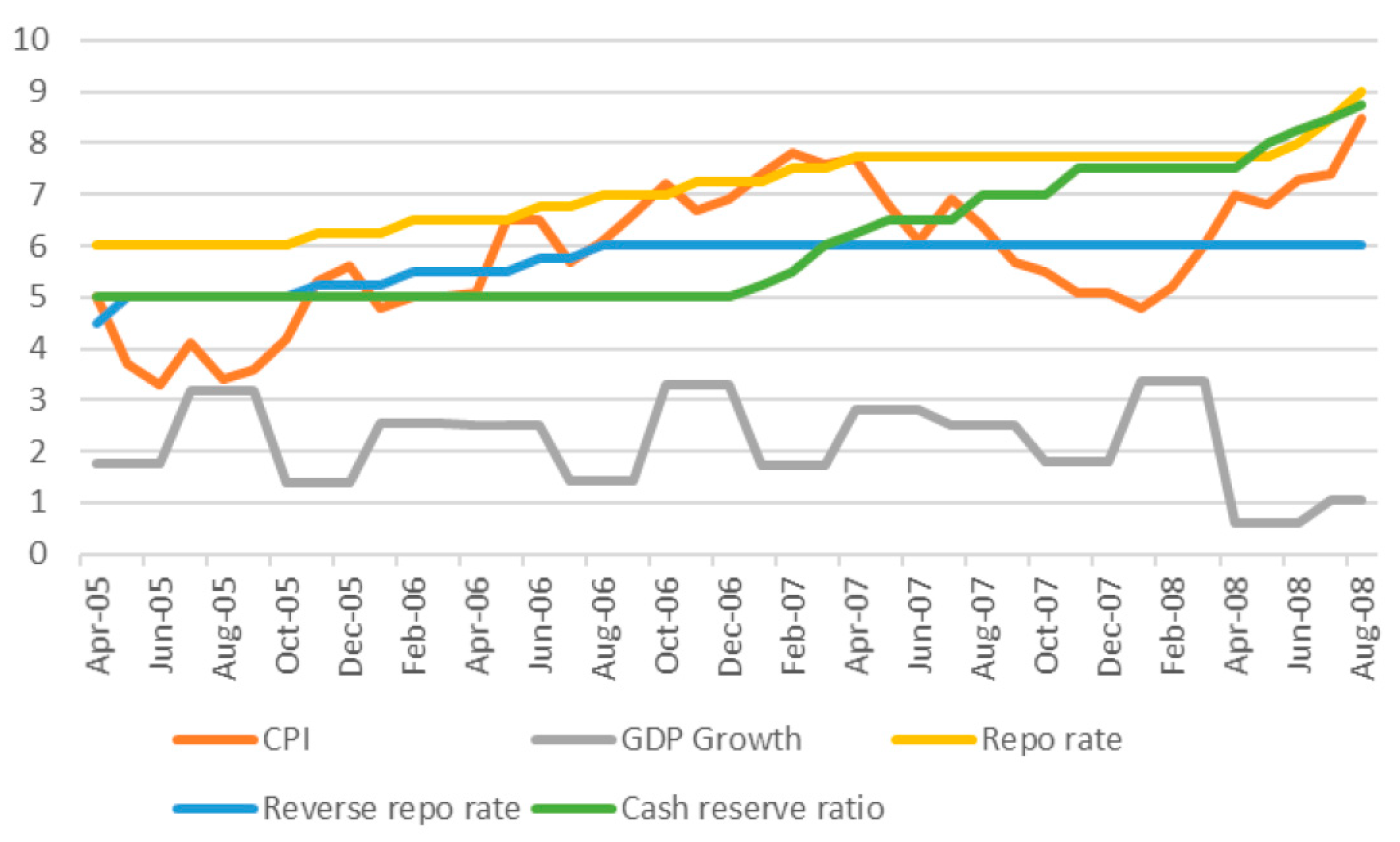
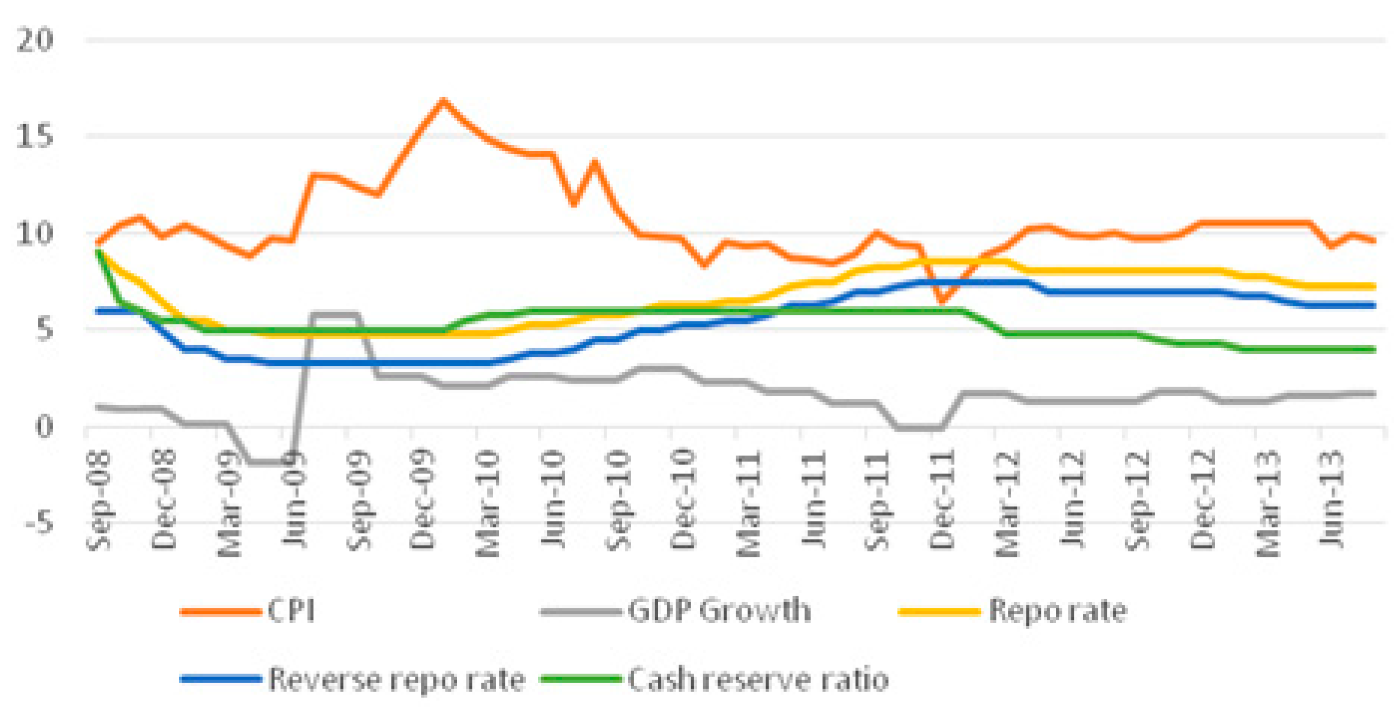
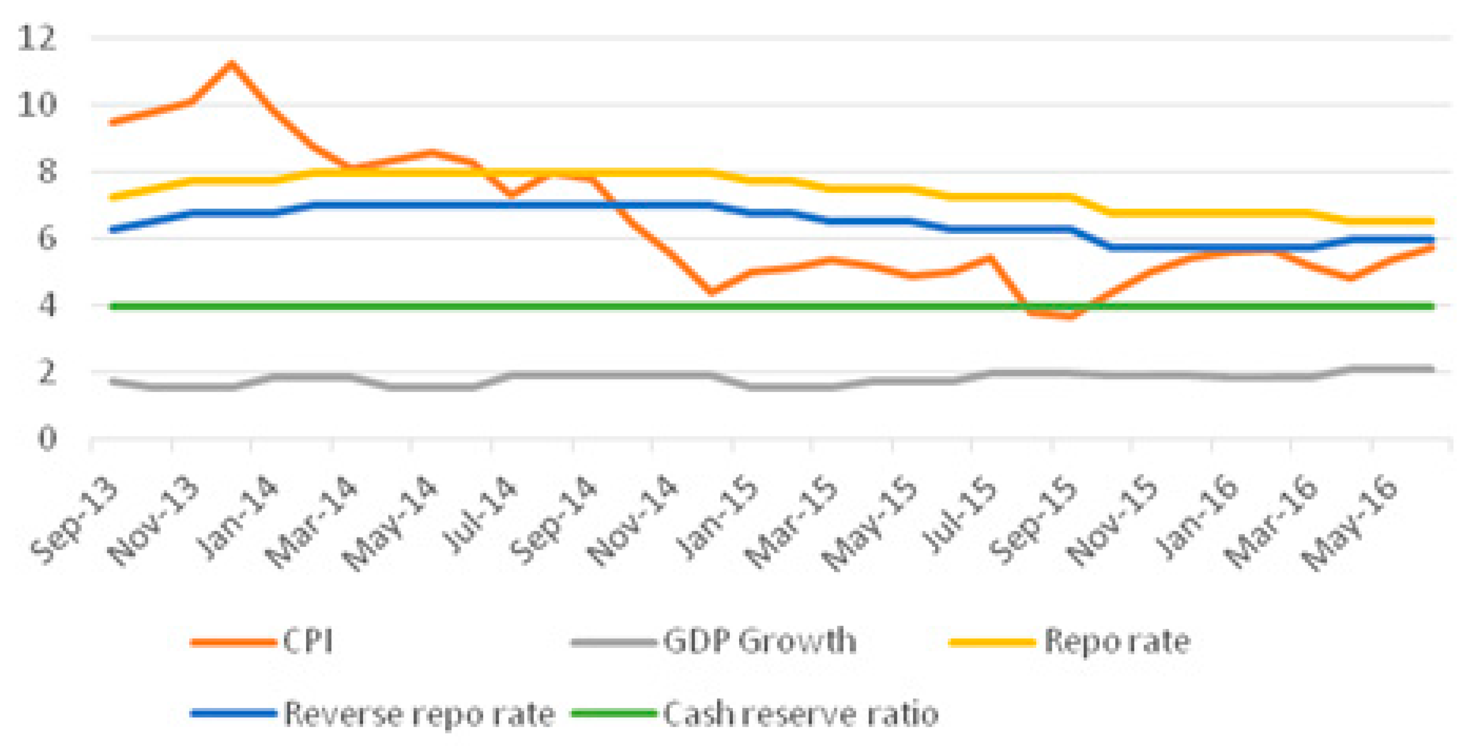
Between 2006 and 2013, the average inflation rate in India was reported to be above 9 per cent. High inflation for such a lengthy period led to public expectations becoming entrenched at high numbers. A rather extended period of low inflation was required to change those expectations;

(b)

Since India shifted focus to CPI from WPI only recently, the public perception of inflation is still largely tied to WPI, which puts weight on internationally traded goods like commodities rather than domestic non-traded goods. As a result, with every dip in international inflation, there was a voice for rate cut. This is primarily why the fight was not taken to the domestic sources of inflation, but Rajan appeared committed to doing so;

(c)

The usual perception is that whenever inflation is low, the central bank should turn to stimulating growth. This is, however, a gross misconception of the workings of a central banking system. Keeping aside the sentimental reactions8 to those, central banking policies work with a lag of 3 to 4 quarters. Therefore, before taking policy decisions, the central bank needs to anticipate how inflation will behave 3 to 4 quarters later. The current rate of inflation, without doubt, provides insights into how it will behave in the future;

(d)

The current inflation, measured on a year on year basis, may be low because there was an unexpected price spurt last year (known as the “base effect”). While evaluating the macro-economic situation through inflation, it is essential to take out the “base effect”, which not everyone may be capable of doing;

(e)

Sources of uncertainty, including the strength and distribution of the monsoon, the extent and persistence of low commodity prices, and the effect of external disturbances on the exchange rate, render the assessment of a future economic situation all the more complex (Rajan 2015b).

Outside observers may not always be able to assess these challenges, and may start forming unrealistic expectations. Rationality of expectations implies that the agents have some idea regarding the anticipated change in policymakers’ decisions as a result of economic evolution (Kydland and Prescott 1977; Ülgen 2009). In tackling inflation and growth challenges, the central bank put great emphasis on unconventional monetary policies. Governor Rajan spelled out his vision of managing the inflation and growth challenges through monetary mechanism during a speech (Rajan 2013b)—

“We are among the large countries with the highest consumer price inflation in the world, even though growth is weaker than we would like it to be… Our households are turning to gold because they find financial investments unattractive… industrial corporations are complaining about high interest rates…

Ultimately, inflation comes from demand exceeding supply, and it can be curtailed only by bringing both in balance. We need to reduce demand somewhat without having serious adverse effects on investment and supply…

…we do need a more carefully spelled out monetary policy framework than we have currently.”

Period 3 witnessed the managing of interest rates by exception, and keeping a close eye on inflation easing. Right from the beginning of the period, the bank had to resist strong demand from the industry and government quarters to cut rates. For instance, Subramanian Swamy, BJP’s Rajya Sabha MP once remarked, “He (Rajan) believes the best way to reduce the temperature of a patient is to kill him,” while Prof Madhav Nalapat, a BJP aide, stated, “He’s good for Wall Street, not for our Main Street” (New York Times 2015a). However, as Rajan observed in his talk “Sustainable Growth in the Financial Sector: 2015 C.K. Prahalad Lecture,” the cause of the politician’s inflation bias was much more mundane.

His central banking policy was largely based on the clarity that bending to such pressure can do more damage than good. Brazil served as a salutary example for him (Rajan 2015c). Until a few years ago, the world was looking towards Brazil as a promising economy with a thriving democracy and continuous reduction in inequalities (The Economist 2016). The country, which witnessed a growth of 7.6 percent in 2010, was contracted by 3.8 percent in 2015 and was predicted to shrink by 2.5–3% in 2016. Many economists argue that Brazil’s troubles have their origins in a series of policy shifts that President Dilma Rousseff pursued once it became clear that the economy was slowing after a burst of growth. Rousseff pressured the central bank to reduce interest rates, fueling a credit spree that overburdened customers struggled to repay (New York Times 2015b). Drawing lessons from the Brazilian crisis, the Reserve Bank of India, in period 3, continued to emphasize minimal interventions and consistent policies for securing long-term growth coupled with reasonable inflation. The Governor (Rajan 2015c) importantly remarked—

“While the Brazilian authorities are working hard to rectify the situation, let us not ignore the lessons their experience suggests. Growth has to be obtained in the right way. It is possible to grow too fast with substantial stimulus, as we did in 2010 and 2011, only to pay the price in higher inflation, higher deficits, and lower growth in 2013 and 2014 … And while monetary policy will accommodate to the extent there is room, we will expand sustainable growth potential only by continuing to implement reforms the government and regulators have announced…”

This strategy was backed by the experts in the field. For instance, Nobel laureate Lars Peter Hansen appreciated the stand to contain inflation against stiff opposition from the industry while maintaining that central banks should continue to focus on controlling inflation (The Times of India 2016). Christine Lagarde, Managing Director of the International Monetary Fund, noted that such selective interventions helped the RBI arrest the surge in gold imports, narrow its current account deficits sharply, and start rebuilding foreign exchange reserves. Lagarde (2015) also lauded the decisive actions taken by RBI during and after the taper tantrum episode by providing foreign currency liquidity support to key sectors, allowing the Rupee to depreciate, and providing judicious foreign exchange interventions to minimize disruptive movements in the Rupee. It is only natural for the financial markets to have responded positively to a stable, transparent, and predictable central banking policy in period 3, as reported in the previous section of this paper.

6. Conclusions

The extant literature has noted that the most direct and immediate effect of changes in central bank policy is on financial markets. Hence, this paper evaluated the performance of financial markets as a result of central banking policies in India during the selected periods, in comparison with other BRICS countries, USA, and UK. Using the country effect model, the paper notes that the financial markets responded positively to the central banking policies in period 3 in India, as compared to period 1 and period 2, and also to the other countries under reference in the same period. The paper also found changes in volatility behavior in financial markets during his tenure.

While evaluating the central banking policy adopted by the Reserve Bank of India in period 3, the paper came out with three major pillars of the underlying philosophy in the form of (a) sticking to the basics; (b) monetary stability and predictability; and (c) handling criticism and pressure. It was found that this philosophy yielded positive results, as India exhibited monetary stability, lowering of inflation, and better growth rates during his tenure. The paper further noted that in period 3, the bank was able to anticipate reality rather than perception while managing his rate cuts. Continued stress of Governor Rajan of lower inflation before effecting rate cuts was based on the need to lower the domestic inflation, inflationary perception of the public, lagged monetary transmission, base effect, and upcoming macro-economic conditions.

References

1. Allison, Paul D. 2009. Fixed Effects Regression Methods. SAGE Publications. Available online: http://www2.sas.com/proceedings/sugi31/184-31.pdf (accessed on 13 October 2018).
2. Andersen, Torben G., Tim Bollerslev, Francis X. Diebold, and Clara Vega. 2007. Real-Time Price Discovery in Global Stock, Bond and Foreign Exchange Markets. Journal of International Economics 73: 251–77. [Google Scholar] [CrossRef]
3. Aziza, Francis Oghenerukevwe. 2010. The Effects of Monetary Policy on Stock Market Performance: A Cross-Country Analysis. SSRN Electronic Journal 2010. [Google Scholar] [CrossRef]
4. Basistha, Arabinda, and Alexander Kurov. 2008. Macroeconomic Cycles and the Stock Market’s Reaction to Monetary Policy. Journal of Banking and Finance 32: 2606–16. [Google Scholar] [CrossRef]
5. Bernanke, Ben S., and Alan S. Blinder. 1992. The Federal Funds Rate and the Channels of Monetary Transmission. American Economic Review 82: 901–21. [Google Scholar] [CrossRef]
6. Bernanke, Ben S., and Kenneth N. Kuttner. 2005. What Explains the Stock Market’s Reaction to Federal Reserve Policy? Journal of Finance 60: 1221–57. [Google Scholar] [CrossRef]
7. Boivin, Jean, and Marc P. Giannoni. 2006. Has Monetary Policy Become More Effective? The Review of Economics and Statistics 88: 445–62. [Google Scholar] [CrossRef]
8. Boivin, Jean. 2006. Has U.S. Monetary Policy Changed? Evidence from Drifting Coefficients and Real-Time Data. Journal of Money, Credit and Banking 38: 1149–73. [Google Scholar] [CrossRef]
9. Bomfim, Antulio N. 2003. Pre-Announcement Effects, News Effects, and Volatility: Monetary Policy and the Stock Market. Journal of Banking and Finance 27: 133–51. [Google Scholar] [CrossRef]
10. Brash, Donald T. 1999. Inflation Targeting: Is New Zealand’s Experience Relevant to Developing Countries? Presented at the Sixth L.K, Jha Memorial Lecture, Mumbai, India, June 17. [Google Scholar]
11. Brooks, Chris. 2008. Introductory Econometrics for Finance. Finance. Cambridge: Cambridge University Press. [Google Scholar] [CrossRef]
12. Brooks, Ray. 1998. Inflation and Monetary Policy Reform. In Australia: Benefiting from Economic Reform. Edited by Anoop Singh, Joshua Felman, Raymond Brooks, Timothy Callen and Christian Thimann. Washington: International Monetary Fund. [Google Scholar]
13. Bryan, Mark L., and Stephen P. Jenkins. 2013. Regression Analysis of Country Effects Using Multilevel Data: A Cautionary Tale. Available online: http://papers.ssrn.com/sol3/papers.cfm?abstract_id=2322088 (accessed on 12 October 2018).
14. Bui, Trung Thanh. 2015. Asymmetric Effect of Monetary Policy on Stock Market Volatility in ASEAN5. Eurasian Journal of Business and Economics 8: 185–97. [Google Scholar] [CrossRef]
15. Chen, Shiu Sheng. 2007. Does Monetary Policy Have Asymmetric Effects on Stock Returns? Journal of Money, Credit and Banking 39: 667–88. [Google Scholar] [CrossRef]
16. Chuliá, Helena, Martin Martens, and Dick van Dijk. 2010. Asymmetric Effects of Federal Funds Target Rate Changes on S&P100 Stock Returns, Volatilities and Correlations. Journal of Banking and Finance 34: 834–39. [Google Scholar] [CrossRef]
17. Clarida, Richard, Jordi Gali, and Mark Gertler. 2000. Monetary Policy Rules and Macroeconomic Stability: Evidence and Some Theory. Quarterly Journal of Economics 115: 147–80. [Google Scholar] [CrossRef]
18. Cogley, Timothy, and Thomas J. Sargent. 2005. Drifts and Volatilities: Monetary Policies and Outcomes in the Post WWII US. Review of Economic Dynamics 8: 262–302. [Google Scholar] [CrossRef]
19. Daly, Kevin. 2008. Financial Volatility: Issues and Measuring Techniques. Physica A: Statistical Mechanics and Its Applications 387: 2377–93. [Google Scholar] [CrossRef]
20. Ehrmann, Michael, and Marcel Fratzscher. 2004. Taking Stock: Monetary Policy Transmission to Equity Markets. Journal of Money, Credit and Banking 36: 719–37. [Google Scholar] [CrossRef]
21. Friedman, Milton. 1968. The Role of Monetary Policy. The American Economic Review 58: 269–95. [Google Scholar] [CrossRef]
22. Goodhart, Charles. 2000. Whither Central Banking? Eleventh C. D. Deshmukh Memorial Lecture. Presented at the 11th C. D. Deshmukh Memorial Lecture, Mumbai, India, December 7. [Google Scholar]
23. Gospodinov, Nikolay, and Ibrahim Jamali. 2012. The Effects of Federal Funds Rate Surprises on S&P 500 Volatility and Volatility Risk Premium. Journal of Empirical Finance 19: 497–510. [Google Scholar] [CrossRef]
24. Guo, Hui. 2004. Stock Prices, Firm Size, and Changes in the Federal Funds Rate Target. Quarterly Review of Economics and Finance 44: 487–507. [Google Scholar] [CrossRef]
25. Ioannidis, Christos, and Alexandros Kontonikas. 2008. The Impact of Monetary Policy on Stock Prices. Journal of Policy Modeling 30: 33–53. [Google Scholar] [CrossRef]
26. Abel, Istvan, and John Bonin. 1992. The ‘big Bang’ versus ‘Slow but Steady’: A Comparison of the Hugarian and Polish Transformations. CEPR Discussion Paper No 626. London: CEPR. [Google Scholar]
27. Jahan, Sarwat, Ahmed Saber Mahmud, and Chris Papageorgiou. 2014. What Is Keynesian Economics? International Monetary Fund 51. [Google Scholar]
28. Jensen, Gerald R., Jeffrey M. Mercer, and Robert R. Johnson. 1996. Business Conditions, Monetary Policy, and Expected Security Returns. Journal of Financial Economics 40: 213–37. [Google Scholar] [CrossRef]
29. Keynes, John Maynard. 1936. The General Theory of Employment, Interest and Money. London: Palgrave Macmillan UK. [Google Scholar]
30. Konrad, Ernst. 2009. The Impact of Monetary Policy Surprises on Asset Return Volatility: The Case of Germany. Financial Markets and Portfolio Management 23: 111–35. [Google Scholar] [CrossRef]
31. Kydland, Finn E., and Edward C. Prescott. 1977. Rules Rather than Discretion: The Inconsistency of Optimal Plans. Journal of Political Economy 85: 473–91. [Google Scholar] [CrossRef]
32. Lagarde, Christine. 2015. Spillovers from Unconventional Monetary Policy—Lessons for Emerging Markets. Presented at the IMF in Reserve Bank of India, Mumbai, India, March 17. [Google Scholar]
33. Lipton, David, and Jeffrey Sachs. 1990. Creating a Market Economy: The Case of Poland. Brookings Papers on Economic Activity 1: 75–147. [Google Scholar] [CrossRef]
34. Lobo, Bento J. 2000. Asymmetric Effects of Interest Rate Changes on Stock Prices. Financial Review 35: 125–44. [Google Scholar] [CrossRef]
35. Martens, Martin, and Dick van Dijk. 2007. Measuring Volatility with the Realized Range. Journal of Econometrics 138: 181–207. [Google Scholar] [CrossRef]
36. Mishra, Prachi, and Raghuram Rajan. 2016. Rules of the Monetary Game. WPS (DEPR). Mumbai: DEPR. [Google Scholar]
37. Mummolo, Jonathan, and Erik Peterson. 2018. Improving the Interpretation of Fixed Effects Regression Results. Political Science Research and Methods, 1–7. [Google Scholar] [CrossRef]
38. Nelson, Daniel B. 1991. Conditional Heteroskedasticity in Asset Returns: A New Approach. Econometrica 59: 347–70. [Google Scholar] [CrossRef]
39. New York Times. 2015a. In India, a Banker in Defense Mode. New York Times, January 15. [Google Scholar]
40. New York Times. 2015b. As a Boom Fades, Brazilians Wonder How It All Went Wrong. New York Times, September 10. [Google Scholar]
41. Patelis, Alex D. 1997. Stock Return Predictability and The Role of Monetary Policy. Journal of Finance 52: 1951–72. [Google Scholar] [CrossRef]
42. Poon, Ser-Huang, and Clive W. J. Granger. 2003. Forecasting Volatility in Financial Markets: A Review. Journal of Economic Literature 41: 478–539. [Google Scholar] [CrossRef]
43. President of the USA. 1975. Economic Report of the President. Washington: United States Government Printing Office. [Google Scholar]
44. Rajan, Raghuram. 2013a. A Step in the Dark: Unconventional Monetary Policy after the Crisis. Presented at the Andrew Crockett Memorial Lecture, Basel, Switzerland, June 23. [Google Scholar]
45. Rajan, Raghuram. 2013b. Speech by Governor Raghuram G. Rajan. Presented at the BANCON 2013, Mumbai, India, November 15. [Google Scholar]
46. Rajan, Raghuram. 2014. Competitive Monetary Easing: Is It Yesterday Once More. Presented at the Central Bank Speech, Brookings Institution, Washington, DC, USA, April 14. [Google Scholar]
47. Rajan, Raghuram. 2015a. Competitive Monetary Easing: Is It Yesterday Once. Macroeconomics and Finance in Emerging Market Economies 8: 2–16. [Google Scholar] [CrossRef]
48. Rajan, Raghuram. 2015b. Strong Sustainable Growth for the Indian Economy. Presented at the FIBAC 2015, Mumbai, India, August 24. [Google Scholar]
49. Rajan, Raghuram. 2015c. Sustainable Growth in the Financial Sector: 2015 C.K. Prahalad Lecture. Presented at the 4th C. K. Prahalad Memorial Lecture, Mumbai, India, September 18. [Google Scholar]
50. Rasche, Robert H, and Marcela M Williams. 2007. The Effectiveness of Monetary Policy. Federal Reserv Bank of St. Louis Review 89: 447–89. [Google Scholar] [CrossRef]
51. Rigobon, Roberto, and Brian Sack. 2003. Measuring the Reaction of Monetary Policy to the Stock Market. Quarterly Journal of Economics 118: 639–69. [Google Scholar] [CrossRef]
52. Su, Chang. 2010. Application of EGARCH Model to Estimate Financial Volatility of Daily Returns: The Empirical Case of China. Master’s thesis, University of Gothenburg, Gothenburg, Sweden. [Google Scholar]
53. Su, Dongwei, and Belton M. Fleisher. 1998. Risk, Return and Regulation in Chinese Stock Markets. Journal of Economics and Business 50: 239–56. [Google Scholar] [CrossRef]
54. The Economic Times. 2017. Guess Who Inspired Raghuram Rajan to Become an Economist? The Economic Times, February 14. [Google Scholar]
55. The Economist. 2016. Brazil’s Fall. The Economist, January 2. [Google Scholar]
56. The Indian Express. 2015. Raghuram Rajan—I Do What I Do. The Indian Express, December 26. [Google Scholar]
57. The Mint. 2008. As the Governor’s Term Ends. The Mint, September 4. [Google Scholar]
58. The Times of India. 2016. Nobel Laureate Backs Raghuram Rajan. The Times of India, July 26. [Google Scholar]
59. The Wire. 2016. Raghuram Rajan’s Legacy at the RBI: Hits, Misses and the Road That Lies Ahead. The Wire, June 19. [Google Scholar]
60. Thorbecke, Willem. 1997. On Stock Market Returns and Monetary Policy. Journal of Finance 52: 635–54. [Google Scholar] [CrossRef]
61. Ülgen, Faruk. 2009. The Credibility of the Central Bank and the Role of Monetary Authorities in a Market Economy. Économie Appliquée 62: 73–98. [Google Scholar]
62. Ülgen, Faruk. 2017. Financial Development, Instability and Some Confused Equations. In Financial Development, Economic Crises and Emerging Market Economies. Edited by Faruk Ülgen. London: Routledge. [Google Scholar]
63. Vähämaa, Sami, and Janne Äijö. 2011. The Fed’s Policy Decisions and Implied Volatility. Journal of Futures Markets 31: 995–1010. [Google Scholar] [CrossRef]
64. Yellen, Janet. 2014. Monetary Policy and Financial Stability. Michel Camdessus Central Banking Lecture at the International Monetary Fund. Washington: International Monetary Fund. [Google Scholar]
65. Zare, Roohollah, M. Azali, and Muzafar Shan Habibullah. 2013. Monetary Policy and Stock Market Volatility in the ASEAN5: Asymmetries Over Bull and Bear Markets. Procedia Economics and Finance 7: 18–27. [Google Scholar] [CrossRef] [Green Version]
1
Brooks (1998) suggests that in the long-run, inflation-targeting countries as a group have improved their rate of economic growth compared to countries which are not inflation-targeters. For a central banker’s opinion about the issue of trade-off between inflation and growth, see Raghuram Rajan’s speech at FIBAC (Rajan 2015b).
2
Throughout this paper, the term ‘financial markets’ is used in a narrower sense and refers to ‘stock markets’ and ‘currency markets’.
3
Raghuram Rajan announced his decision not to seek the second term, on Saturday, 18 June 2016. Therefore, the paper considers his period till 17 June 2016 only. For the purpose of the study ‘period 3’ ranges from 5 September 2013 through 17 June 2016.
4
The Indian Express (“Raghuram Rajan—I Do What I Do”. The Indian Express, 26 December 26 2015) maintains that central banking is much more than monetary policy. Raghuram Rajan, in his speech at BANCON 2013 held at Mumbai on 15 November 2013, outlined five developmental measures of RBI—
a.
Clarifying and strengthening the monetary policy framework;
b.
Strengthening banking structure through new entry, branch expansion, encouraging new varieties of banks, and moving foreign banks into better regulated organisational forms.
c.
Broadening and deepening financial markets and increasing their liquidity and resilience so that they can help allocate and absorb the risks entailed in financing India’s growth.
d.
Expanding access to finance to small and medium enterprises, the unorganised sector, the poor, and remote and underserved areas of the country through technology, new business practices, and new organisational structures; that is, we need financial inclusion.
e.
Improving the system’s ability to deal with corporate distress and financial institution distress by strengthening real and financial restructuring as well as debt recovery.
For the purpose of this paper, we use the term ‘central banking policy’ in a narrower sense and refer to points ‘a’ and ‘c’ above.
5
Brooks (1998) suggests that in the long-run, inflation-targeting countries as a group have improved their rate of economic growth compared to countries which are not inflation-targeters. For Raghuram Rajan’s opinion about the issue of trade-off between inflation and growth, see his speech at FIBAC (Rajan 2015b).
6
‘Monetarism’ is an economic school of thought that gained popularity in the 1960s and 1970s and presented a theoretical challenge to Keynesian economics. Milton Friedman is regarded as the founding father of ‘monetarism’.
7
For a more detailed discussion on shock therapy and gradual approach, and the need for distinctive policies in emerging economies, see (Ülgen 2017).
8
During his speech at FIBAC, Rajan (2015a) interestingly remarked, “the central bank is not a “cheerleader” for the economy. By this I did not mean that the RBI does not want to do its utmost to see the economy do well. Far from it! What I meant is that it is not the role of the central bank to elevate sentiments unduly, to deliver booster shots to the stock market so that it can soar for a while, only to collapse when reality hits.”
Figure 1. Consumer Price Index (CPI), gross domestic profit (GDP), and policy interventions during ‘period 1’.
Economies 07 00049 g001
Figure 2. CPI, GDP, and policy interventions during ‘period 2’.
Economies 07 00049 g002
Figure 3. CPI, GDP, and policy interventions during ‘period 3’.
Economies 07 00049 g003