Source Country Economic Development and Dynamics of the Skill Composition of Emigration

Abstract

This paper presents an endogenous growth model of migration and technological diffusion with transitional dynamics, which provide explanations for the empirical pattern of the mobility transition. A two-skill group extension of this model offers new hypotheses regarding the skill composition of emigration during the mobility transition. Skill-biased technological change (SBTC), which first occurs in the destination, raises the relative return to high skill migration and thus the high-to-low skill emigration ratio. As SBTC eventually diffuses to the source economy, it also raises the relative return to high skill investment there, and causes a decline in the high-to-low skill emigration ratio. Empirical evidence using bilateral migration data from 31 destinations and 195 origins is shown to support this hypothesis, with the average income of origins, at which the peak high-to-low skill emigration ratio is reached, is estimated at $2000 in 2011 US dollars PPP (adjusted for purchasing power parity). Furthermore, research and development intensity as a measure of SBTC in destinations is shown to be empirically, positively linked to the bilateral high-to-low skill emigration ratio.

1. Introduction

Data on emigration from 195 economies—where the migrants were born (source or origin countries)—to 30 developed destination countries members of the Organization for Economic Co-operation and Development (OECD)—where the migrants reside collected by Docquier and Marfouk (2006)—indicate that the share of college educated emigrants increased from 1990 to 2000 from 29.8% to 34.6% of the total stock of foreign born. However, the emigration rates of college educated migrants from source countries with different development levels and who migrated to these OECD destinations varied in 2000 from 6.1% for low income origins, to 7.6% for lower-middle income origins, 7.9% for upper-middle income origins, and 3.5% for high income origins.

Recent empirical studies on the impact of economic development in source countries on emigration have brought evidence in support of the theory of the mobility transition as first introduced by Zelinsky (1971). This theory suggests that during the initial phases of economic development in source countries emigration rates increase with average income, while after a threshold level of income is reached, emigration rates decrease. These empirical studies, including (Vogler and Rotte 2000); (Telli 2014); (Clemens 2014); (Djajic et al. 2016) and (Dao et al. 2018), have analyzed the greater variety and quality of international migration data, which have become available in the last two decades, to find that the rate of emigration traces an inverted-U path as source countries’ incomes increase. These results add an important new dimension to the long supported hypothesis that emigration linearly declines with economic development in source countries.

However, what is the impact of economic development in source countries on the skill composition of emigration, and what are the channels through which continuing source economy development leads to changing migrant skill levels? While these changes can be due to both a changing skill structure within the source economy as well as the resulting skill selection of migrants due to altered costs and benefits of migration along the development transition, the role of economic development in determining the skill composition of emigration has not been researched systematically in the literature.

Few recent exceptions include Djajic et al. (2016), who find that the ratio of high-to-low skill emigrants is decreasing with wages in the source country, a pattern they explain through the role played by credit constraints in the migration decision. Dao et al. (2018) show that the upward sloped segment of the mobility transition is largely explained by the increasing share in the source country and in emigration flows of highly skilled individuals. McKenzie and Rapoport (2010) present empirical evidence that migrants from communities with small migrant networks in destinations tend to be positively selected, while those from communities with large migrant networks are negatively selected.

In a review of the mobility transition literature over the previous 45 years, Clemens (2014) groups theoretical explanations into six categories, including explanations based on credit constraints, the demographic transition, information asymmetries, structural change, income inequality, and immigration barriers abroad. Although the mobility transition hypothesis primarily concerns the total emigration rate as economic development advances, in each one of these theory classes, human capital plays an important role. However, only few of these theories have addressed the implications of economic development for the migration decisions of differently skilled individuals despite the fact that economic development also impacts returns to skills as well as the costs and benefits of emigration for individuals of different skill levels.

Previous research on the relation between economic growth and emigration has primarily focused on the brain drain effect, which analyzes the impact of skilled emigration on income, human capital, and overall economic development in source countries. Studies in this area have analyzed both positive and negative effects of skilled emigration, introducing the theoretical and empirical possibility of a brain gain impact on source economies (Mountford 1997; Beine et al. 2001; Chen 2009; Beine et al. 2011).

In an endogenous growth model with endogenous migration outcomes, Cipriani (2006) analyzes differences in fertility rates between migrants and non-migrants, and also finds that the more highly skilled have a greater likelihood of migrating due to their increased ability to cover the costs of migration, and that the skill selection of migrants linearly decreases as the technology level of the destination economy increases. Larramona and Sanso (2006) also employ an endogenous growth model with migration decisions to analyze the impact of emigration on source countries. The theoretical analysis presents steady state and transitional dynamics of the impact of migration on growth, and shows that income differences between source and destination economies can be maintained at the steady state while migration flows at a constant rate. However, they do not discuss the differences in migration outcomes for differently skilled workers.

Technological diffusion from developed economies has played an important role in developing countries’ economic growth (Keller 2004), but differences in the intensity of adoption still explain a large share of income differences between rich and poor countries (Comin and Mestieri 2018). Technological change since the 1980s has been increasingly skill biased especially through the development of information and communication technologies which have disproportionately raised the productivity of and demand for highly skilled workers, as well as the return to skills in both developed (Katz and Autor 1999) and developing economies (Conte and Vivarelli 2011). However, as the technology transfer to developing countries has occurred with a lag and imperfect intensity, it has also contributed to maintaining differences in returns to skills between developed and developing countries (Vivarelli 2014). Berman and Machin (2000) document that mainly middle income countries experience diffusion of skill-biased technology. Thus the disparity in returns to skill is higher especially in the beginning of the economic development transition, creating stronger incentives for higher skill workers to migrate to developed economies when income at home is relatively low. Fadinger and Mayr (2014) show that source countries with higher skill ratios have lower rates of high skill emigration and suggest skill-biased technological change (SBTC) as the explanation for this relation. However, they do not trace the dynamic relationship between economic development in source countries and the emigration of differently skilled individuals.

This study is the first to present an endogenous economic growth model, which explains the empirical pattern of the mobility transition as an endogenous outcome resulting from migration decisions in which investment in human capital is a central motivating force. In this overlapping generations model, economic development and migration outcomes are determined jointly, and are dynamically linked. Parents make decisions about family migration influenced not only by the relative potential earnings in the destination economy, but also by the relative rate of return on investment in the human capital of their children. In this setup, factors which impact earnings and returns to educational investments like technological progress, skill-biased technological change (SBTC), and technological diffusion from more advanced economies, become central. Theoretical results show that mobility transition can be generated by either of two factors associated with economic development: a permanent decrease in the time cost of migration and technological progress, respectively. An additional skill heterogeneous model extension presents new hypotheses regarding the impact of SBTC on the skill composition of emigration during the mobility transition, while novel empirical results provide support for these hypotheses.

Important contributions brought by this model compared to earlier endogenous growth and emigration models include an analysis of the central role of SBTC in explaining the mobility transition and its skill composition, along with the dynamic transitional analysis of endogenous emigration rates by skill level during the economic development transition. Differences in demands for skills between source and destination economies due to SBTC which initially occurs in developed countries and later diffuses to developing ones, result in the high-to-low skill emigration ratio first rising and then, after a threshold level of income, declining along the mobility transition.

This paper also presents empirical evidence in support of the hypothesis of an inverted-U path of the high-to-low skill emigration ratio during the economic development of source countries by using bilateral migration data by educational attainment for 31 developed destinations and 195 origins from Docquier et al. (2009). The migration data span the 1990–2000 decade thus capturing a period of high economic growth in developed destination economies due to high rates of innovation and adoption of Information and Communication Technologies, and their implicit skill bias, a period during which intensifying international trade between developed and developing countries also contributed to increased international diffusion of these technologies.

The structure of the paper is as follows: Section 2 presents the endogenous growth model in a representative agent setup which is used to generate the mobility transition pattern, while Section 3 extends the model to a two-agent skill heterogeneous framework in which further results are presented relating to the skill composition of emigration along the mobility transition; Section 4 presents the empirical analysis and estimation results, Section 5 discusses the policy implications of these results, and Section 6 concludes.

2. Migration Dynamics during Economic Development

This section presents a general equilibrium endogenous growth model of migration and development in which human capital is the engine of growth, and where knowledge diffuses from a technological leader to a technological follower economy through human capital externalities. The benchmark model presented in this section is an extension of the endogenous growth and heterogeneous-skill agent closed economy model of Ehrlich and Kim (2007) to a two-country setup with the addition of endogenous migration decisions and flows connecting the two economies. Working age adults make decisions regarding human capital investment, fertility, and where to reside, migrating in response to utility differences between the leader and follower economies, until these differences are eliminated. Without loss of generality, migrants are assumed to only move in one direction, from the follower to the leader economy, based on utility differences.

2.1. Model Setup

Human capital in each economy before migration occurs in period t is $h_{t,c}$, and population before migration is $N^n{}_{t,c}$, where the upper script n stands for native population and the subscript c stands for the country: L for the technological leader, and F for the technological follower. The number of migrants is given by $M_t$, the emigration rate out of the follower economy is $m_{t,F}=\frac{M_t}{N^n{}_{t,F}}$, while the immigration rate into the leader economy is $m_{t,L}=\frac{M_t}{N^n{}_{t,L}}$.

2.1.1. Production

Final goods production is given by the following Cobb–Douglas function:

$$Y_{t,c}=D_c{\left(N^e{}_{t,c}\right)}^{\alpha }{\left(P_c\right)}^{1-\alpha }{\left({\overline{h}}_{t,c}\right)}^{\rho }$$

(1)

where $N^e{}_{t,c}={\overline{l}}_{t,c}{N}_{t,c}{\overline{h}}_{t,c}$ is effective labor supply, ${\overline{l}}_{t,c}$ is average labor supply, $N_{t,c}$ is total population, ${\overline{h}}_{t,c}$ is average human capital, and parameters are such that $0<\alpha ,\rho <1$ and $\alpha +\rho >1$. P_c represents the endowment level of country-specific public resources, and D_c represents total factor productivity (TFP). The production function exhibits decreasing returns to scale with respect to effective labor and public resources, and increasing returns to scale to human capital through positive externalities from the average level of human capital. Under these conditions, the production function in Equation (1) satisfies the Inada conditions with respect to the main two inputs into production, effective labor and public resources, which are sufficient for a study of long run growth.

2.1.2. Labor and Public Resource Markets

The equilibrium wage rate per unit of effective labor in each economy equals the marginal productivity of effective labor: $w_{t,c}=\frac{\partial Y_{t,c}}{\partial N^e{}_{t,c}}=D_c\alpha {\left(N^e{}_{t,c}\right)}^{\alpha -1}{\left({\overline{h}}_{t,c}\right)}^{\rho }{\left(P_c\right)}^{1-\alpha }$. The rental rate of the public resource is determined through a public auction where firms compete as they bid on the quantity and rental rate of the public resource they want to employ in production. The equilibrium rental rate per unit of public resource employed is the marginal productivity of the public resource: $r_{t,c}=\frac{\partial Y_{t,c}}{\partial P_c}=D_c\left(1-\alpha \right){\left(P_c\right)}^{-\alpha }{\left(N^e{}_{t,c}\right)}^{\alpha }{\left({\overline{h}}_{t,c}\right)}^{\rho }$. The revenue collected through this auction when all of the country’s public resources are employed, $r_{t,c}\cdot P_c$, is paid to households in proportion to their effective labor supply. Thus, total household income per unit of effective labor from wages and transfer payments is:

$$w^e{}_{t,c}=w_{t,c}+\frac{r_{t,c}{P}_c}{N^e{}_{t,c}}=D_c{\left(P_c\right)}^{1-\alpha }{\left({\overline{l}}_{t,c}{N}_{t,c}\right)}^{\alpha -1}{\left({\overline{h}}_{t,c}\right)}^{\alpha +\rho -1}$$

(2)

For a simplified notation, from now $w_{t,c}$ will denote the effective wage rate as laid out in Equation (2).

2.1.3. Altruism, Fertility, and Human Capital Investment

The utility of a working age individual takes the logarithmic form:

$$u^r{}_{t,c}=\ln c^r{}_{t,c}+\delta \cdot \ln a^r{}_{t+1,c}$$

(3)

where r(resident) = n (ative) or m (igrant), and δ is the intertemporal discount factor. Utility depends on the adult’s current consumption, c^r_t,c, and an altruism term, a^r_t+1,c, which depends positively on the welfare of the individual’s children in the next period. Individuals live two time periods: when young spending time attaining human capital, and when of working age deciding how to divide their available time between working, child rearing, children’s human capital investment, and migrating. Adults have a total amount of time available normalized to 1, of which l_t,c represents time spent working at the market clearing wage rate, w_t,c. Rearing children has a constant time cost of v_c per child, and the rate of fertility is denoted as n_t,c. Parents also spend time educating their children, where e_t,c represents time spent educating each child, with a constant time cost factor of θ_c. Migration has a time cost of $\tau$. Thus, the budget constraint in period t for an individual with human capital level h_t,c is given by:

$$c^r{}_{t,c}=l^r{}_{t,c}{w}_{t,c}{h}^r{}_{t,c}=\left(1-v_c{n}^r{}_{t,c}-{\theta }_c{n}^r{}_{t,c}{e}^r{}_{t,c}-migr\cdot \tau \right)w_{t,c}{h}^r{}_{t,c}$$

(4)

where the term migr equals 1 for a migrant, and 0 for a non-migrant.

Human capital accumulation is given by $h^r{}_{t+1,c}={\lambda }_c{e}^r{}_{t,c}{S}_{t,c}{}^{\gamma }{h}^r{}_{t,c}$, where λ_c is the productivity of educational investments in the respective country, and S_t,c^γ is a positive externality term from the relative human capital of the leader economy, given by $S_{t,c}=\frac{{\overline{h}}_{t,L}{N}_{t,L}}{{\overline{h}}_{t,c}{N}_{t,c}}$. The role of this externality term is to model the diffusion of knowledge and technology from the leader to the follower economy, with countries farther apart in total levels of human capital experiencing greater diffusion, which allows for a catching up process to occur through a faster growth rate. Poncet and Fouquin (2006) documents that countries at lower levels of total factor productivity (TFP) experienced higher growth rates of TFP in the preceding decade and a half. Migrant human capital accumulation also benefits from the higher educational productivity of human capital in the leader economy: $h^m{}_{t+1,L}={\lambda }_L{e}^m{}_{t,L}{S}_{t,L}{}^{\gamma }{h}_{t,F}$. The altruism function is:

$$a^r{}_{t+1,c}=b{\left(n^r{}_{t,c}\right)}^{\beta }{h}^r{}_{t+1,c}$$

(5)

Through this specification, adult parents care about the number of children they have with an elasticity factor of β > 0, and linearly about the human capital of their children.

2.2. Optimization: Fertility, Human Capital Investment, and Migration

Optimal fertility, human capital investment, and migration rates are obtained through a two-step approach. Taking each distinct group’s decision separately, non-migrant residents of the follower, native residents of the leader, and migrants, optimal fertility and human capital investment rates are obtained from utility maximization conditions. Given optimal rates determined in the first step, the equilibrium migration rate is the one that equalizes the indirect utilities of residing in the follower and leader economies, respectively, for a migrant.

The utility function in Equation (3) is maximized by each of the three groups of adults with respect to fertility and educational investment, and subject to the budget constraint in Equation (4) and the altruism function in Equation (5), yielding the following optimal conditions1^,2:

$$n^r{}_c=\frac{\delta \left(\beta -1\right)\left(1-migr\cdot \tau \right)}{\left(1+\delta \beta \right)v_c}$$

(6)

$$e_c=\frac{v_c}{{\theta }_c\left(\beta -1\right)}$$

(7)

Migrants and natives residing in the leader economy find it optimal to invest the same amount of time in their children’s education, but more than parents in the follower economy due to higher time cost of rearing children and lower time cost of education. Migrant parents have lower optimal fertility than natives in the source country due to v_L > v_F, and also lower than natives in the leader economy due to the disruption effect of migration.

Potential migrants take wages and the external effect as given when deciding whether to migrate. Given optimal fertility and educational investment decisions from Equations (6) and (7), the indirect utility of a non-migrant native of the follower economy is a function of the equilibrium wage rate in the follower economy and the external effect: $V_{t,F}=\ln \left(\frac{w_{t,F}{h}_{t,F}}{1+\delta \beta }\right)+\delta \ln \left[b{\left(\frac{\delta \left(\beta -1\right)}{\left(1+\delta \beta \right)v_F}\right)}^{\beta }\frac{{\lambda }_F{v}_F}{{\theta }_F\left(\beta -1\right)}{S}_{t,F}{}^{\gamma }{h}_{t,F}\right]$. The indirect utility of a migrant resident of the leader economy has a similar form: $V^m{}_{t,L}=\ln \left(\frac{\left(1-\tau \right)w_{t,L}{h}_{t,F}}{1+\delta \beta }\right)+\delta \ln \left[b{\left(\frac{\delta \left(\beta -1\right)\left(1-\tau \right)}{\left(1+\delta \beta \right)v_L}\right)}^{\beta }\frac{{\lambda }_L{v}_L}{{\theta }_L\left(\beta -1\right)}{h}_{t,F}\right]$. As long as V^m_t,L > V_t,F, residents of the follower economy find it beneficial to migrate to the leader economy. As labor supplies change in the two economies due to migration, wages, and the return to human capital investment through spillovers in the follower economy rise, while wages in the leader economy fall, thus lowering the utility differential. The equilibrium immigration rate at each time t, m_t,L, is the immigration rate that ensures

$$V^m{}_{t,L}\left(m_{t,L}\right)=V_{t,F}\left(m_{t,L}\right)$$

(8)

Given that $\frac{\partial w_{t,F}}{\partial m_{t,L}}>0$, $\frac{\partial S_{t,F}}{\partial m_{t,L}}>0$, and $\frac{\partial w_{t,L}}{\partial m_{t,L}}<0$ implies that $\frac{\partial V^m{}_{t,L}}{\partial m_{t,L}}<0$ and $\frac{\partial V_{t,F}}{\partial m_{t,L}}>0$ monotonically, meaning that Equation (8) has a unique solution for m_t,L.

2.3. The Steady State

Definition 1.

A steady state is a set of optimal human capital investment, fertility, and migration rates,${\left\{e^r{}_c,n^r{}_c,m_c\right\}}_{c=F.L}^{r=n,m}$, such that rates of growth of human capital and population are constant in each country.

Positive steady state emigration and immigration rates are sustained in this model due to a higher level of TFP, average human capital, educational efficiency of human capital, and lower fertility in the leader economy.

Proposition 1.

The inter-country knowledge spillover term,$S_{t,F}$, ensures that the rates of growth of human capital in the two economies converge in the long run to the same constant value.

Proposition 2.

The migration process leads in the long run to a constant relative wage ratio between the two countries. As a result, migration between the two economies leads to the equalization of population rates of growth.

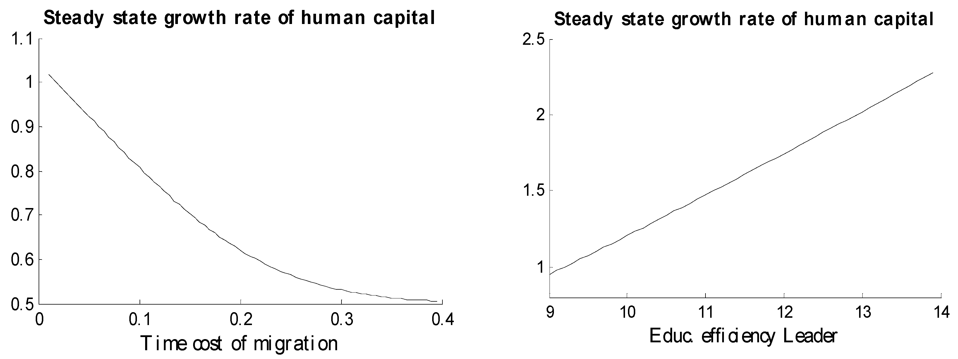
The ensuing analysis will center on growth steady states, which are achieved when the educational efficiency of human capital in the leader economy is high enough to sustain positive growth in the average level of human capital in the long run. This occurs when parameters are such that $\frac{h_{t+1,L}}{h_{t,L}}={\varphi }_L\frac{1+m{*}_L\left(1-\tau \right)\frac{1}{X*}}{1+m{*}_L\left(1-\tau \right)}>1$, where $X_t\equiv \frac{h_{t,L}}{h_{t, F}}$ and ${\varphi }_c\equiv \frac{{\eta }_c{v}_c}{\left(\beta -1\right)}{\left(S_c*\right)}^{\gamma }$, while stars indicate steady state values.

Under these conditions, a one-time permanent decrease in the time cost of migration, $\tau$, achieved either through changes in migration policy that make it easier to migrate or as related to advancements in transportation or communication technology, raises the long run rate of growth of human capital in both countries, $g_h^{*}$. The increase in the relative population ratio, $Z_t\equiv \frac{N_{t,L}}{N_{t,F}}$, which occurs in the transitional period due to higher transitional migration leads to higher inter-country educational spillovers which increase $g_h$. Thus, as a larger proportion of skilled individuals work in the technologically advanced economy, growth rises in both the leader and follower economies due to the respective human capital spillovers3. This relation is illustrated in Figure 1 through numerical simulation.

The educational efficiency of the leader economy, ${\eta }_L$, is positively related to $g{*}_h$. An increase in ${\eta }_L$ which can be due to technological progress directly increases the long run growth rate of human capital in the leader economy, and through educational spillovers also the growth rate in the follower economy. Numerical simulation in Figure 1 shows this relation.

2.4. Transition Paths of Migration and Growth during Economic Development

An economy is undergoing a development transition when it is on a path from a regime with a low growth rate to a regime with a higher growth rate of human capital. This section analyzes the transitional paths of migration during development transitions triggered by a decrease in the time cost of migration, τ, and separately by an increase in the educational efficiency of human capital in the leader economy, ${\eta }_L$. These results provide dynamic endogenous growth explanations for the empirically documented mobility transition.

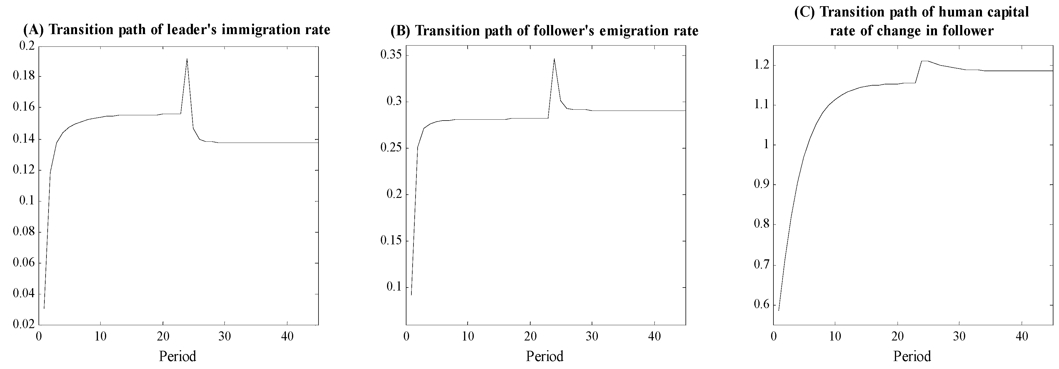
Under the first type of development trigger, a decrease in τ, the emigration, $m_{t,F}$, and immigration, $m_{t,L}$, rates initially increase, raising $Z_t$. This in turn lowers the relative wage rate in the next period, which causes $m_{t,L}$ and $m_{t,F}$ to decrease. Along the development transition, $m_{t,L}$ and $m_{t,F}$ continue to decrease toward the new steady state. Numerical simulations of the transitional paths of $m_{t,L}$, $m_{t,F}$, and the growth rate of human capital as a result of a permanent decrease in τ are illustrated in Figure 2.

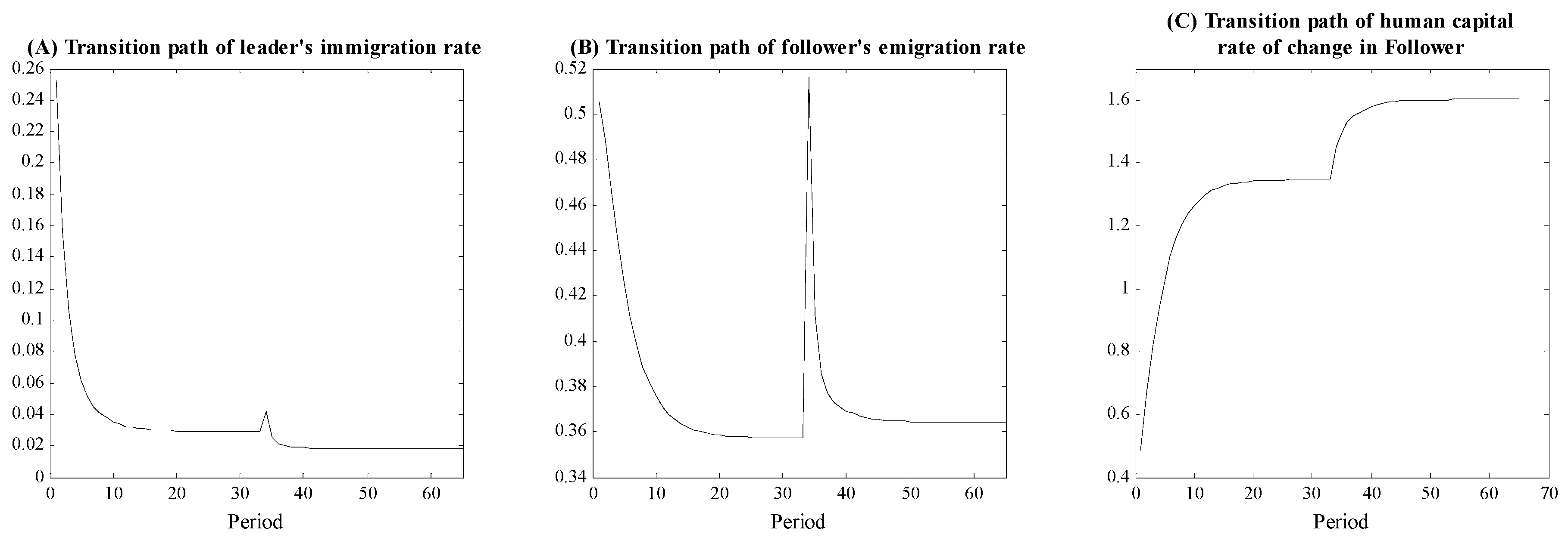
Proposition 3.

If$\alpha +\rho -1<\delta \gamma$4 and$e_{m_{t,L},Z_t}<-1$, where$e_{m_{t,L},Z_t}$is the elasticity of$m_{t,L}$with respect to$Z_t$, a one-time permanent decrease in τ leads to inverted-U paths of$m_{t,L}$and$m_{t,F}$over the ensuing development transition.

An increase in ${\eta }_L$ initially raises the return to migration by increasing the rate of return to investment in education relative to the follower economy, causing $m_{t,L}$ and $m_{t,F}$ to increase. In the following period, higher rates of migration raise $Z_t$ causing the relative wage rate to decrease. As a result, $m_{t,L}$ and $m_{t,F}$ start to decrease toward the new steady state. Numerical simulations of the transitional paths of $m_{t,L}$, $m_{t,F}$, and the growth rate of human capital as a result of a permanent increase in ${\eta }_L$ are illustrated in Figure 3.

Proposition 4.

If$\alpha +\rho -1>\delta \gamma$and$e_{m_{t,L},Z_t}<-1$, a one-time permanent increase in${\eta }_L$leads to inverted-U paths of$m_{t,L}$and$m_{t,F}$over the ensuing development transition.

Propositions 3 and 4 illustrate how a decrease in the time cost of migration as well as an increase in educational efficiency in the leader economy, both of which also trigger an economic development transition, lead to an inverted-U shaped path of the emigration rate as documented in the mobility transition empirical literature.

3. The Skill Composition of Migration during Economic Development

To analyze the dynamics of the skill composition of migration during economic development, this section extends the model from Section 2 to a two-skill group model.

3.1. The Two-Skill Group Model: Setup and Optimization

Production functions for the high and low skill sectors are given separately by $Y_{t,c}^i=D_c{\left(N_{t,c}^{i,e}\right)}^{\alpha }{\left(P_c^i\right)}^{1-\alpha }{\left({\overline{h}}_{t,c}^i\right)}^{\rho }$, where i = 1 for the high skill group, and 2 for the low skill group. Under the same assumptions about the functioning of labor and resource markets as in Section 2, these production functions yield the following skill specific wage rates:

$$w_{t,c}^i=D_c{\left(P_c^i\right)}^{1-\alpha }{\left({\overline{l}}_{t,c}^i{N}_{t,c}^i\right)}^{\alpha -1}{\left({\overline{h}}_{t,c}^i\right)}^{\alpha +\rho -1}$$

(9)

Utility takes the logarithmic form $u_{t,c}^{i,r}=\ln \left(c_{t,c}^{i,r}\right)+\delta \ln \left(a_{t+1,c}^{i,r}\right)$, where $i=1,2;r=n,m;c=F,L$. The consumption and altruism terms are now group specific: $c_{t,c}^{i,r}=l_{t,c}^{i,r}{w}_{t,c}^i{h}_{t,c}^{i,r}=\left(1-v_c{n}_{t,c}^{i,r}-{\theta }_c^i{e}_{t,c}^{i,r}{n}_{t,c}^{i,r}-mig{r}_c^i\cdot \tau \right)w_{t,c}{h}_{t,c}^{i,r}$ and $a_{t+1,c}^{i,r}=b{\left(n_{t,c}^{i,r}\right)}^{\beta }{h}_{t+1,c}^{i,r}$. Skill specific human capital accumulation is given by $h_{t+1,c}^{i,r}={\lambda }_c^i{e}_{t,c}^{i,r}{\left(S_{t,c}^{i,D}\right)}^{{\gamma }_1}{\left(S_{t,c}^{i,G}\right)}^{{\gamma }_2}{h}_{t,c}^{i,r}$, where $S_{t,c}^{i,D}=\frac{{\overline{h}}_{t,c}^1{N}_{t,c}^1}{{\overline{h}}_{t,c}^i{N}_{t,c}^i}$ is the domestic spillover term which benefits the lower skill group in each economy from the total human capital of the higher skill group in the same economy, and $S_{t,c}^{i,G}=\frac{{\overline{h}}_{t,L}^i{N}_{t,L}^i}{{\overline{h}}_{t,c}^i{N}_{t,c}^i}$ is the global spillover term which benefits skill group i in the follower economy from the total human capital of skill group i in the leader economy.

Optimal educational investment and fertilities are given by: $e_c^i=\frac{v_c}{{\theta }_c^i\left(\beta -1\right)}$ and $n_c=\frac{\delta \left(\beta -1\right)}{\left(1+\delta \beta \right)v_c}$. Given the indirect utilities for each group and in each country, the following are the migration equations that imply the equalization of indirect utilities at the equilibrium migration rates for each skill group:

$$\frac{w_{t,L}^i}{w_{t,F}^i{\left(S_{t,F}^{i,G}\right)}^{\delta {\gamma }_2}}\cdot {\left(\frac{S_{t,L}^{i,D}}{S_{t,F}^{i,D}}\right)}^{\delta {\gamma }_1}={\left[{\left(\frac{v_L}{v_F}\right)}^{\beta -1}\frac{{\eta }_F^i}{{\eta }_L^i}\right]}^{\delta }{\left(1-\tau \right)}^{-1-\delta \beta }$$

(10)

3.2. The Steady State

Definition 2.

A steady state is a set of optimal skill group specific human capital investment, fertility, and migration rates,${\left\{e_c^{i,r},n_c^{i,r},m_c^{i,r}\right\}}_{c=F.L}^{r=n,m}$, such that skill group specific migration rates, rates of change of human capital, and population are constant.

Proposition 5.

The skill specific relative native human capital ratio,$X_t^i$, and the skill specific relative native population ratio,$Z_t^i$, converge to constant values in the steady state.

3.3. Developing the Transitional Path of the Skill Composition of Migration

SBTC occurring in the leader economy, modeled through an increase in ${\eta }_L^1$, triggers a development transition in both countries by initially raising the educational efficiency of high skill educational investment in the leader economy and then diffusing to the follower. Human capital spillovers then also raise the efficiency of low skill educational investment in the leader economy in the following period, as well as the efficiency of educational investment of both skill groups in the follower economy, albeit with a smaller magnitude.

Proposition 6.

An increase in the educational efficiency of human capital of the high skill group in the leader economy, ${\eta }_L^1$, triggers a development transition in both economies towards a steady state with a higher rate of growth of average human capital.

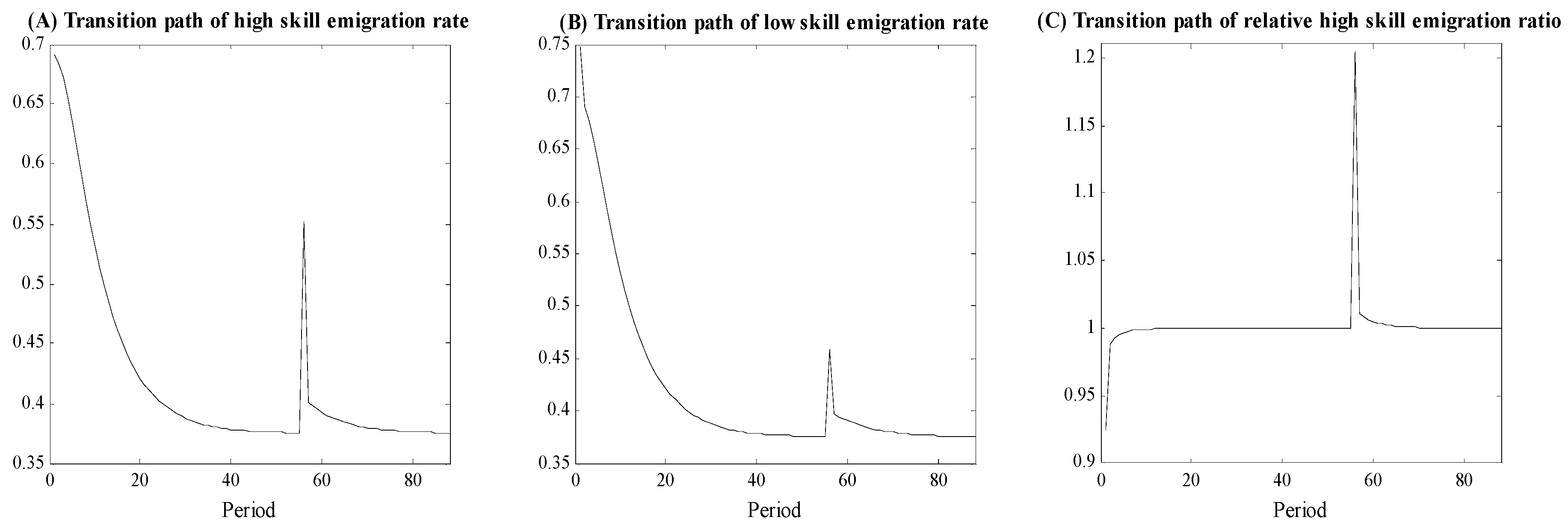
A higher ${\eta }_L^1$ raises the return to migration for high skill workers by increasing the return to educational investment for this group in the leader economy. The high skill emigration rate, $m_{t,F}^1$, and immigration rate, $m_{t,L}^1$, thus increase, but start decreasing in the following period as the initial flow of high skill workers lowers the leader’s relative high skill wage rate. The high skill group has the initial and largest incentive to migrate as a result of SBTC occurring in the leader economy at the beginning of the development transition. Through human capital spillovers, the relative return to educational investment for the low skill group in the leader economy also increases initially thus raising $m_{t,F}^2$ and $m_{t,L}^2$, but with a lower magnitude due to γ₁ < 1 and γ₂ < 1. In the following period, $m_{t,F}^2$ and $m_{t,L}^2$ start to decrease due to a decrease in the low skill relative wage rate in the leader economy.

Proposition 7.

If$\alpha +\rho -1>\delta \left({\gamma }_1+{\gamma }_2\right)$5 and$e_{m_{t,L}^i,Z_t^i}<-1$, during the economic development transition triggered by an increase in${\eta }_L^1$,$m_{t,F}^1,m_{t,F}^2$, and the high-to-low skill emigration ratio,$\frac{m_{t,F}^1}{m_{t,F}^2}$, follow inverted-U paths.

Numerical simulations illustrating the transitional paths of $m_{t,F}^1,m_{t,F}^2$ and $\frac{m_{t,F}^1}{m_{t,F}^2}$ as a result of a permanent increase in ${\eta }_L^1$ are shown in Figure 4.

The results of Proposition 7 indicate that SBTC, which initiates in the leader economy, can trigger both an economic development transition as well as a mobility transition during which human capital and income rise faster in both countries and the skill selection of emigration from the follower economy rises in the first part of this transition and falls in the latter part.

4. Empirical Analysis

This section presents empirical tests of the results of Proposition 7, regarding changes in the skill composition of emigration during the economic development transition and the role of SBTC diffusion as a channel through which economic development impacts the emigrant skill mix. The main hypothesis to be tested states that (1) the high-to-low skill emigration ratio follows an inverted-U path as the income of source economies rises during economic development. Additional hypotheses arising from the results of Proposition 7 were also tested. These hypotheses state that (2) during the economic development of source economies, the high skill and low skill emigration rates also follow inverted-U paths, but that (3) the changes in the low skill emigration rate over the same transitional period have smaller magnitudes than those of the high skill emigration rate, and (4) that SBTC in destination economies has a positive impact on the high-to-low skill emigration ratio.

To test the above stated hypotheses, this section uses migration, development, and SBTC data for the 1990–2000 period, which represents an ideal setting for the testing of the theoretical results. As the world was growing in interconnectedness with rising rates of migration, fast advancements in computer and Internet technologies increased demand for highly skilled workers in developed countries and was also diffusing to middle income countries.

4.1. Empirical Model

To test the main hypothesis from Proposition 7 empirically, the following equation models the high-to-low skill bilateral emigration ratio as a quadratic function of the level of economic development of origins, along with additional controls:

$$\ln \left(E{M}_{i,j}\right)=\alpha +{\beta }_1\ln \left(y_i\right)+{\beta }_2{\left[\ln \left(y_i\right)\right]}^2+{\beta }_3\ln \left(y_j\right)+{\beta }_4\ln \left(d_{i,j}\right)+{\beta }_5{p}_j+{\beta }_6\ln \left(po{p}_i\right)+\gamma X_{i,j}+\theta Z_{i,j}+e_{i,j}$$

(11)

where i is the source and j is the destination, $E{M}_{i,j}$ is the bilateral high-to-low skill emigration ratio from country i to country j, $y$ represents the income per person before migration, $d_{i,j}$ is the bilateral physical distance between source and destination, $p_j$ is a policy variable for the degree to which the destination’s immigration policy favors the highly skilled, pop_i is the total population in the origin, $X_{i,j}$ is a vector of three bilateral dummy variables for contiguity, common language, and historical colonial relations between the source and the destination, $Z_{i,j}$ is a vector of two dummy variables for the destination and the source, respectively, which control for destination and source fixed effects, while $e_{i,j}$ is the i.i.d. error term. Testing the results of Proposition 7 suggests a null hypothesis H₀: ${\beta }_1\le 0$ or ${\beta }_2\ge 0$, and an alternative hypothesis H₁: ${\beta }_1>0$ and ${\beta }_2<0$.

The dependent variable, $E{M}_{i,j}$, measures the bilateral high-to-low skill emigration ratio:

$$E{M}_{i,j}=\frac{1+m_{i,j}^H}{1+m_{i,j}^L},m_{i,j}^S=\frac{S_{i,j,t+1}^S-S_{i,j,t}^S}{R_{i,t}^S}$$

(12)

where $m_{i,j}^S$ is the net bilateral emigration rate of skill level S which can be either high, H, or low, L, from country i to country j, $S_{i,j,t}^S$ represents the bilateral stock of migrants from country i residing in country j at time t of skill level s, and $R_{i,t}^s$ represents the resident population of skill level s in the source country i at time t before migration occurs. The dependent variable from Equation (11) is calculated using high and low skill net emigration rates as flow rather than stock variables in order to capture the changing migration incentives during the economic development transition. A value of 1 is added to each emigration rate when calculating $E{M}_{i,j}$ to account for negative values of net emigration rates. Thus, the origin is experiencing positive skill selection of bilateral emigration when $E{M}_{i,j}>1$, and negative selection when $E{M}_{i,j}<1$.

Estimating Equation (11) using ordinary least squares (OLS) could yield biased coefficient estimates due to the endogeneity of the level of economic development in determining the skill composition of migration. The endogeneity is created by the simultaneity of these two variables, given that the average income and the skill composition of migration are joint outcomes of the economic development process, as described in the theoretical analysis. As the skill selection of emigration rises with income at low levels of income in origins it would also in turn cause average income in origins to decrease if human capital per worker in the source country declines as a result of increasingly skilled emigration. While when the skill selection of emigration falls with income in origins, the reverse causation channel would be expected to lead to an increase in average income if increasingly less skilled emigration raises human capital per worker. This suggests that OLS estimates would have a downward bias.

I addressed this endogeneity issue in two ways. First, I used the average income per person in origins and destinations before migration occurs. This lag attempts to exclude the reverse causation impact of emigration on income in the source country. I also used instrumental variable estimation by employing the share of urban population in an economy before migration occurs as an instrument for average income. The urban share in an economy is positively correlated with the level of economic development, but not in itself a determinant of future international migration rates except through the impact of economic development. Furthermore, the bilateral structure of the estimation equation includes origin and destination fixed effects, which help control for unobservable and missing variables specific to each country.

To test Hypotheses (2) and (3) stated above, I also estimated Equation (11) using the high skill bilateral emigration rate and low skill bilateral emigration rate in turn as dependent variables. To test hypothesis (4), I estimated the impact of SBTC in destination economies on the bilateral high-to-low skill emigration ratio, as well as on the bilateral high skill and low skill emigration rates separately using the following equation:

$$\begin{array}{l}\ln \left(E{M}_{i,j}\right)=a+{\gamma }_{1}SBT{C}_i+{\gamma }_{2}SBT{C}_j+{\lambda }_1\ln (skillpre{m}_i)+{\lambda }_2\ln (skillpre{m}_j)+{\delta }_1\ln \left(y_i\right)+{\delta }_2\ln \left(y_j\right)\\ +{\eta }_{1}urba{n}_i+{\eta }_{2}urba{n}_j+\chi \ln \left(d_{i,j}\right)+\phi p_j+\varphi \ln \left(po{p}_i\right)+\nu X_{i,j}+\rho Z_{i,j}+{\epsilon }_{i,j}\end{array}$$

(13)

where skillprem is the skill premium, urban represents the level of urbanization of an economy, ${\epsilon }_{i,j}$ represents the i.i.d. error term, and the rest of the variables are defined the same as for Equation (11).

4.2. Data and Sources

Data on the educational attainments of foreign born residents in 30 OECD countries and South Africa are from Docquier et al. (2009). The educational attainment categories reported in this dataset are primary, secondary, and tertiary education, and the data corresponds to two census rounds from destinations, 1990/91 and 2000/01. With as many as 195 source countries, this data set provided a large variation in economic development levels of origins over which the skill composition of migration was analyzed. The high skill group included all those over 25 with at least some tertiary education. Data on the resident population’s distribution of educational attainments in 1990 also came from Docquier et al. (2009). Average income in source and destination economies in 1990 was proxied by real GDP per capita values adjusted for purchasing power parity (PPP) from Feenstra et al. (2015). 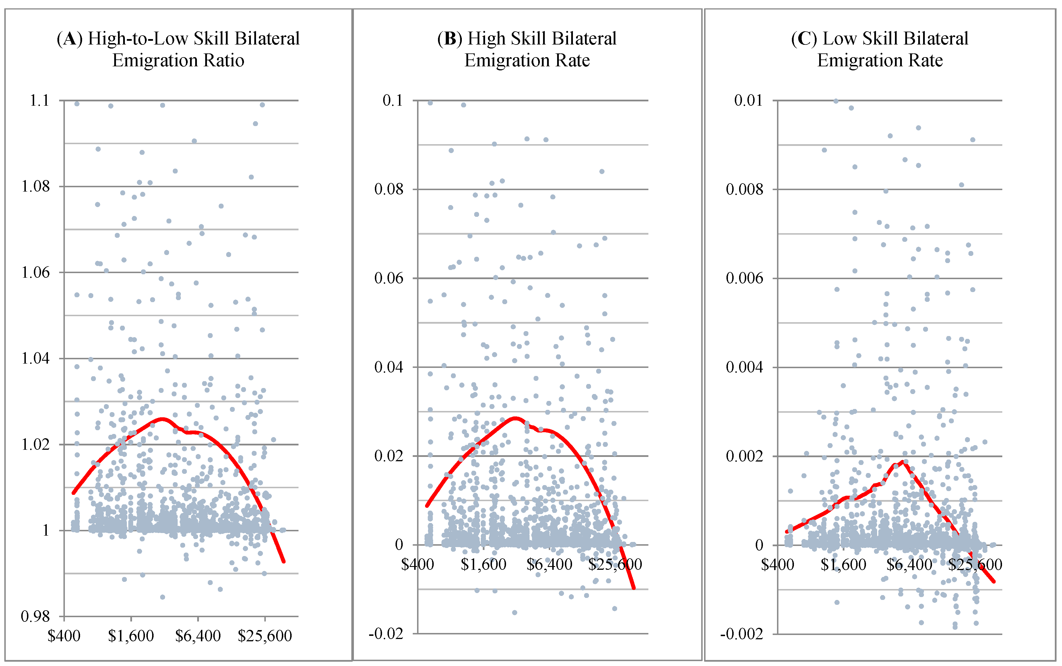Figure 5 shows in panel A the non-parametric regression fitting using lowess smoothing of the relationship between the bilateral high-to-low skill emigration ratio, $E{M}_{i,j}$, and the level of economic development in origins measured by the real GDP per capita in 1990. The estimated non-parametric relationship shows that at low levels of income, the share of highly skilled workers who emigrate to a given destination is higher than that of low skilled emigrants, and rising as income initially rises. The high-to-low skill bilateral emigration ratio reaches a peak at an income level of about $3000 in 2011 PPP US dollars, after which the ratio starts to decline until at income levels above $28,000, the share of low skill workers that emigrate becomes higher than that of high skill emigrants. At its peak, the high-to-low skill bilateral emigration ratio suggests that the high skill bilateral emigration rate is about 2.6 percentage points higher than the low skill bilateral emigration rate. Panels B and C show similar relationships between the high and low skill bilateral emigration rates and origins’ GDP per capita. The high skill bilateral emigration rate rises faster, reaches the peak at a lower income level, and then also falls faster than the low skill bilateral emigration rate. The non-parametric estimated relations depicted in Figure 5 support Hypotheses (1)–(3) stated above arising from the results of Proposition 7 from the theoretical analysis.

The bilateral distance, along with bilateral variables on common language, colonial relations, and contiguity are from Mayer and Zignago (2011). Information on the degree to which immigration policies in destinations favored highly skilled workers during the period 1990–2000 is from McLaughlan and Salt (2002) and Lowell (2005). I compose a discrete policy variable to characterize the degree to which a host economy facilitates the immigration of highly skilled workers, with 0 being assigned to countries with no specific policies, 0.2 to those with limited work permits for specific skills and industries (Denmark, France, and Germany), and 1 assigned for broader policies intended to attract the highly skilled (Australia, Canada, Japan, South Korea, New Zealand, United States). The share of research and development (R&D) spending as a percentage of GDP serves as a proxy for SBTC. Data on R&D expenditure as a percentage of GDP (R&D intensity) were from The World Bank (2018) and were averaged over 1996–2000. Gini index data averaged over the 1995–2005 period from the World Income Inequality Database were employed as proxy for the skill premium. Data on the share of the population that lives in urban areas in 1990 were also from The World Bank (2018).

4.3. Estimation Results

The results of the ordinary least squares (OLS) and instrumental variables (IV) estimations for Equation (11) are presented in

Table 1. Skill selection of bilateral emigration and source country economic development ^a.

Explanatory Variables	OLS			IV
	Dependent Variable
	(1) ln of High-to-Low Skill Bilateral Emigration Ratio	(2) ln of High Skill Bilateral Emigration Rate	(3) ln of Low Skill Bilateral Emigration Rate	(4) ln of High-to-Low Skill Bilateral Emigration Ratio	(5) ln of High Skill Bilateral Emigration Rate	(6) ln of Low Skill Bilateral Emigration Rate
Ln source GDP per capita	0.0988 ** (0.0469)	0.1114 ** (0.0535)	0.0125 * (0.0073)	0.1406 ** (0.0646)	0.1542 ** (0.0728)	0.0136 (0.0094)
Ln source GDP per capita, squared	–0.0062 ** (0.0029)	–0.0070 ** (0.0033)	–0.0008 * (0.0004)	–0.0092 ** (0.0042)	–0.0101 ** (0.0047)	–0.0009 (0.0006)
Ln destination GDP per capita	0.0175 (0.0111)	0.0189 (0.0121)	0.0014 (0.0012)	0.0043 (0.0103)	0.0029 (0.0113)	–0.0013 (0.0018)
Destination high skill immigration policy	0.0358 *** (0.0136)	0.0394 *** (0.0152)	0.0036 ** (0.0018)	0.0413 *** (0.0159)	0.0454 ** (0.0178)	0.0041 * (0.0021)
Adjusted-R2	0.1845	0.1853	0.0689	0.1830	0.1830	0.0638
Observations	2795	2795	2795	2780	2780	2780

^a Each specification includes dummy variables for contiguity, common language, and colonial relations, as well as the natural logarithm of the bilateral distance and of the total population over 25 in the source in 1990. Fixed destination and source effects are included in all specifications. Cluster correlation and heteroskedasticity robust standard errors are in parentheses. *, **, and *** refer to p-values of 10%, 5%, and 1%, respectively.

in columns (1) and (4), respectively. The IV results present estimates employing as instruments the share of urban population of source and destination economies for the respective countries’ level of development. The coefficient estimates for ${\beta }_1$ and ${\beta }_2$ have the expected signs under both OLS and IV models, with ${\widehat{\beta }}_1>0$ and ${\widehat{\beta }}_2<0$, both being statistically significant at 5% under both models. Coefficient estimates for the high skill bilateral emigration rate and low skill bilateral emigration rate are also presented in Table 1 under OLS in columns (2) and (3), and IV estimation in columns (5) and (6). The estimated coefficients for both relations display the expected signs, with the estimated coefficients for the high skill bilateral emigration rate statistically significant at a 5% level under both OLS and IV, and the estimated coefficients for the low skill bilateral emigration rate significant only at 10% under the OLS model. The coefficients for origin income and origin income squared show larger magnitudes in the IV estimation than in OLS, indicating a potential downward bias in OLS estimation as expected when considering the two way causation of emigration and economic development. These results support Hypotheses (1), (2), and (3) derived from the theoretical analysis.

The strength of the instruments used is tested using the Cragg–Donald weak instrument test, which is reported in

Table 2. First stage results of IV estimation ^b.

Explanatory Variables	Dependent Variable
	Ln Source GDP per Capita	Ln Destination GDP per Capita
Ln source urban share	1.2421 *** (0.0216)	-
Ln destination urban share	-	1.3908 *** (0.3673)
Adjusted-R2	0.5309	0.3576
F-test (Cragg-Donald)	1,693,800 ***
Observations	2780

^b Each specification includes all exogenous variables used in the main regressions from Table 1. Cluster correlation and heteroskedasticity robust standard errors are in parentheses unless otherwise specified. *** refer to p-values of 10%, 5%, and 1%, respectively.

. The Cragg–Donald statistic rejects the null hypothesis of weak instruments in at 1% significance level. In addition, t statistics on each instrument confirm the strength of instruments at a 1% confidence level.

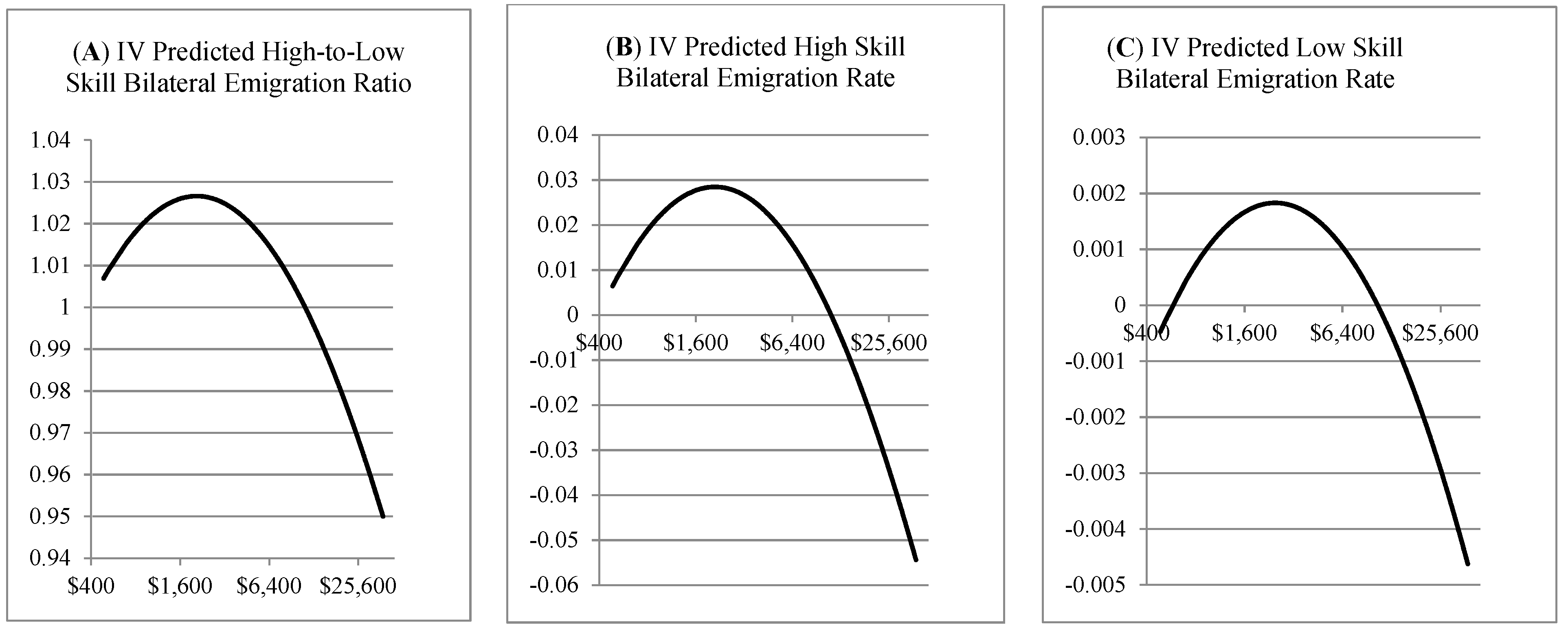
Figure 6 illustrates the partial estimated relationships between origins’ GDP per capita and (1) the predicted high-to-low skill bilateral emigration ratio, (2) the predicted high skill bilateral emigration rate, and (3) the predicted low skill bilateral emigration rate, based on the IV coefficient estimates in columns (4), (5), and (6), respectively, from Table 1. Figure 6A shows a peak value for the predicted path of the high-to-low skill bilateral emigration ratio at an average income of $2082 in 2011 PPP US dollars. Figure 6B illustrating the high skill bilateral emigration rate, shows a peak at an average income value of $2067, while the predicted low skill bilateral emigration rate in Panel C reaches a peak at $1911. The predicted high skill bilateral emigration rate rises to higher values and later falls to lower values than the predicted low skill emigration rate, which supports the theoretical results from Proposition 7. The IV estimated coefficients suggest that at the peak high-to-low skill emigration ratio, the high skill bilateral emigration rate is about 2.7 percentage points higher than the low skill bilateral emigration rate, which is consistent with the prediction from the non-parametric lowess estimation.

Among the 164 origins included in the regression analysis, Ghana, Senegal, Kenya, and Egypt had average real GDP per capita values in the range 1900–$2100 in 1990. Two of the largest migrant origins and fastest developing nations, India and China, fell close to the left and right of the estimated peak for the high-to-low skill emigration ratio respectively, with an average GDP per capita in 1990 of about $1300 for India and about $2400 for China. The peak skill selection of emigration is predicted to occur before the median income value of $5890 for the origins considered in this analysis.

Table 3. Skill selection of bilateral emigration and research and development (R&D) intensity ^c.

OLS	Dependent Variable
	ln of High-to-Low Skill Bilateral Emigration Ratio	ln of High Skill Bilateral Emigration Rate	ln of Low Skill Bilateral Emigration Rate
Source R&D Intensity	0.0010 (0.0009)	0.0011 (0.0010)	0.0001 (0.0003)
Destination R&D Intensity	0.0029 ** (0.0014)	0.0032 ** (0.0016)	0.0003 (0.0003)
Ln source Gini index	0.0123 * (0.0070)	0.0147 * (0.0088)	0.0024 (0.0005)
Ln destination Gini index	0.0185 ** (0.0079)	0.0208 ** (0.0090)	−0.0023 (0.0008)
Ln source GDP per capita	0.0008 (0.0016)	0.0002 (0.0018)	−0.0006 (0.0016)
Ln destination GDP per capita	0.0067 * (0.0034)	0.0076 ** (0.0038)	0.0009 (0.0016)
Source urban share	−0.0002 * (0.0001)	−0.0002 * (0.0001)	0.0000 (0.0002)
Destination urban share	−0.0001 (0.0001)	−0.0001* (0.0001)	−0.0000 (0.0016)
Destination high skill immigration policy	0.0081 ** (0.0039)	0.0097 ** (0.0046)	0.0016 * (0.0011)
Adjusted-R2	0.1342	0.1335	0.0362
Observations	1782	1782	1782

^c Each specification includes dummy variables for contiguity, common language, and colonial relations, as well as the natural logarithm of the bilateral distance and of the total population over 25 in the source in 1990. Cluster correlation and heteroskedasticity robust standard errors are in parentheses. * and ** refer to p-values of 10%, 5%, and 1%, respectively. Fixed destination and source effects are included in all specifications.

shows results for the estimated impact using OLS on the skill levels of emigrants of R&D intensity in destination and source economies after controlling for the skill premium in those countries. R&D intensity in destinations has a positive estimated effect on the high-to-low skill bilateral emigration ratio as well as on the high skill bilateral emigration rate, and the coefficient estimates are both significant at the 5% level. These coefficient estimates suggest that every additional 1% of GDP spent on R&D in destinations is associated with an additional 0.3% of high skill bilateral emigration. The effect of the skill premium in destinations is estimated to be positive and statistically significant at 5% on both dependent variables. These results support the hypothesis from the theoretical analysis that SBTC in destination economies, as proxied here by R&D intensity, creates incentives for increased skilled migration in addition to the incentives created by a higher skill premium in destinations.

The impact of R&D intensity in both origins and destinations on the low skill bilateral emigration rate is estimated to be positive but not statistically significant and with about a ten times smaller magnitude than the coefficients for high skill emigration. In the same model, the skill premium of origins has a positive estimated impact, while the skill premium of destinations has a negative estimated impact, although both are not statistically significant. These results are also supportive of the results of Proposition 7, as they suggest a more muted impact of SBTC on low skill emigrants separate from the impact of the skill premium.

5. Policy Implications

The results of this research suggest that low income countries embarking on the development transition will experience an increase in the share of highly skilled among emigrants with the peak skill selection at a lower-middle income level. The implications for government policy in these countries is that investment in education would need to be larger to compensate for the brain drain experienced by the economy. However, the results from this study also suggest that the benefits to middle income countries from opening their economies to international trade and finance to a greater degree include the possibility of faster SBTC diffusion which would cause increasingly less of the highly skilled to leave. In addition, as middle income countries continue to develop, the skill selection of emigration is shown to eventually decline thus relieving part of the cost burden of brain drain.

Immigration quotas set by developed countries often do not favor lower income origins, but the results of this study suggest the largest source economies for skilled migrants are low to lower-middle income countries. This also implies that tailoring immigration policy to different origins based on the predicted pattern of skill selection over the course of economic development could more effectively address labor resource demands in destinations. Since skilled migrants are shown to respond to incentives related to SBTC in destinations, well-targeted immigration policy could thus help alleviate existing skilled worker shortages in fields where SBTC is present destination economies.

6. Conclusions

Recent empirical studies have brought new evidence in support of the mobility transition pattern as first hypothesized by Zelinsky (1971). Such evidence raises the question of the channel through which economic development in source countries causes the emigration rate to first increase, and after a threshold level of income to decrease. Credit constraints, the skill composition of residents in the source country, and migrant networks have been suggested in previous studies as explanations for the empirical pattern of the mobility transition and its skill composition. This paper highlights the role of SBTC both theoretically and empirically. Within a skill heterogeneous endogenous growth model, SBTC which first occurs in developed destination economies causes the return to high skill investment to rise there and trigger an increase in emigration from developing source countries, primarily the emigration of higher skilled individuals. Once SBTC starts to diffuse to developing source countries later in the economic development process, the relative return to high skill investment in destinations falls and causes a decline in overall emigration as well as in the high-to-low skill emigration ratio. In addition, this study presents empirical evidence in support of the inverted-U path of the high-to-low skill emigration ratio during the economic development of source countries using bilateral migration data from 31 destinations and 195 origins. The average income of origins at which the peak high-to-low skill emigration rate is predicted to occur is around $2000 in 2011 PPP US dollars. The empirical analysis also identifies R&D intensity in destinations as a factor that is positively linked to the bilateral high-to-low skill emigration ratio, thus supporting the hypothesis that SBTC in destinations triggers higher relative emigration of the highly skilled.