Investigating Spillover Effects between Foreign Exchange Rate Volatility and Commodity Price Volatility in Uganda

Abstract

This study investigates the impact of commodity price volatility spillovers on financial sector stability. Specifically, the study investigates the spillover effects between oil and food price volatility and the volatility of a key macroeconomic indicator of importance to financial stability: the nominal Uganda shilling per United States dollar (UGX/USD) exchange rate. Volatility spillover is examined using the Generalized Vector Autoregressive (GVAR) approach and Multivariate Generalized Autoregressive Conditional Heteroskedasticity (MGARCH) techniques, namely the dynamic conditional correlation (DCC), constant conditional correlation (CCC), and varying conditional correlation (VCC) models. Overall, the results of both the GVAR and MGARCH techniques indicate low levels of volatility spillover and market interconnectedness except during crisis periods, at which point cross-market volatility spillovers and market interconnectedness sharply and markedly increased. Specifically, the results of the MGARCH analysis show that the DCC model produces the best results. The obtained results point to an amplification of dynamic conditional correlations during and after the global financial crisis (GFC), suggesting an increase in volatility spillovers and interdependence between these markets following the global financial crisis. This is also confirmed by the results of the total spillover index based on the GVAR analysis, which shows low but time-varying volatility spillover that intensified during periods of high uncertainty and market crises, particularly during the global financial crisis and sovereign debt crisis periods.

1. Introduction

Over the years, growing integration and globalization has made the world’s economy more interdependent. This interdependence in part reflects the success of decades of liberalization efforts, and is largely the result of expansion, diversification, and the deepening of trade and financial links between countries enhanced by technological developments. In the 1980s, many African governments initiated liberalization efforts as part of structural adjustment programs aimed at promoting economic development. The resulting integration into the world economy not only raised the living standards in many African countries, but also saw the rapid proliferation of telecommunication technology, the globalization of business activity, and increased policy and regulatory coordination.

Although economic integration has yielded numerous benefits, the resulting global interdependency of markets and economies has made countries more vulnerable to fluctuations in prices in the world market and global economic shocks in general. There is growing evidence that mean and volatility spillovers occur between asset markets; that is, events in one market can be transmitted to others, and that the magnitude of such interrelationships may be strengthened during crisis periods. African economies are particularly susceptible to this exposure and vulnerability, given their economic dependence on foreign markets and aid arising from the export of a few primary commodities, structural problems, and weak institutions and policy frameworks (IMF 2003; Varangis et al. 2004). Since commodity prices are volatile and subject to frequent shocks, commodity-dependent countries are frequently exposed to large deteriorations in their current account, which may create broader distress across the rest of the economy, compromising financial stability and setting back growth gains that have already been achieved.

Indeed, external shocks such as commodity price fluctuations are often highlighted as one of the major reasons for macroeconomic instability and the poor economic performance of African countries (IMF 2003; Raddatz 2007; Varangis et al. 2004). However, Raddatz (2007) found that external shocks, including commodity price fluctuations, explain only a small fraction of the output variance of low-income countries, which includes most sub-Saharan African countries, while other factors—most likely internal causes—are the main source of fluctuations. Nevertheless, the effects of commodity price volatility on output and macroeconomic stability may vary across regions and countries, depending on the duration of the shock, the economic significance of the commodity for the country in question, and whether it is a net importer or exporter of this commodity (IMF 2003; UNCTAD 2012; Varangis et al. 2004).

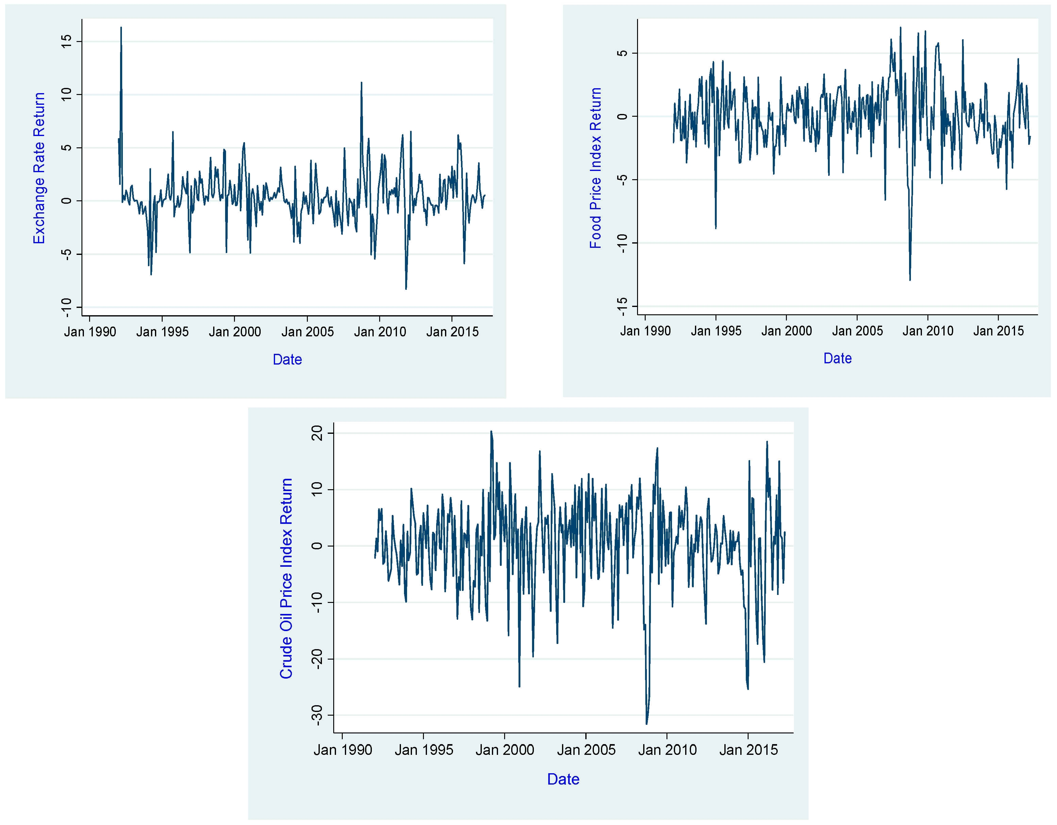
Consequently, understanding the country-specific dynamics of volatility spillovers in international commodity prices on financial stability is important from a policy perspective, especially if appropriate policies that maximize the potential benefits from globalization and minimize the downside risks of destabilization are to be developed. For instance, an understanding of spillover dynamics may inform global policy coordination efforts, as well as inform central banks’ foreign exchange market intervention efforts aimed at maintaining financial sector stability, especially during crisis periods. This notwithstanding, the existing literature provides a paucity of empirical evidence on the effects of commodity price volatility on financial stability in developing countries. This paper undertakes to fill this gap in the extant literature by investigating volatility spillovers between commodity prices and macroeconomic indicators of importance regarding financial stability in Uganda. Specifically, the study investigates the spillover effects of oil and food price volatility on the volatility of a key macroeconomic indicator of importance to financial stability, the nominal Uganda shilling per United States dollar (UGX/USD) exchange rate. The study focuses on the UGX/USD exchange rate, mainly because it accounts for a majority of foreign currency transactions in the Ugandan economy. To the best of our knowledge, this is the only study that investigates the spillover effects between commodity price volatility and financial sector stability in the context of Uganda. The rest of study is organized as follows: Section 2 presents a brief overview of the Ugandan financial sector stability; Section 3 provides a brief review of the literature, while Section 4 presents the methodology applied. Empirical results are provided in Section 5, and conclusions with recommendations are drawn in Section 6.

2. Overview of Financial Sector Stability

Undeniably, Uganda’s rapid economic growth in the past was in part supported by key reforms in the financial sector, including the liberalization of domestic financial markets and the removal of quantitative controls on credit. Indeed, Uganda’s prudent macroeconomic management resulted in a consistent record of impressive performance, as evidenced by the average gross domestic product (GDP) growth rates of 7.4%, single digit inflation averaging at 6.5% and an improved external position with an average current account deficit as a percent of GDP of 4.3% in the period of 2001 to 2010 (World Bank 2015). However, in the recent past, the country has witnessed more economic volatility, and GDP growth slowed to an average of just about 5% (World Bank 2016).

The importance of a sound and well-functioning financial system in facilitating the mentioned outcomes in economic growth above cannot be understated. As such, the maintenance of price stability and a sound financial system remains at the core of Bank of Uganda’s mission (Bank of Uganda 2016). In line with international best practice, the Bank of Uganda’s regulatory and supervisory framework encourages innovation and efficient competition in financial services based on prudent risk taking and the avoidance of reckless bank management. Until the late 1990s, Uganda’s financial sector was predominantly small and fragile due to a combination of misguided financial policies pursued by successive governments along with severe macroeconomic and political instability (Henstridge and Kasekende 2001; Whitworth and Williamson 2010). During this period, the financial sector recorded severe incidences of crisis and distress, including episodes of hyperinflation, which resulted in severe financial disintermediation. In an effort to address these weaknesses, the country undertook extensive reforms in the financial sector in the 1990s, including the liberalization of financial markets, restructuring distressed banks, and strengthening prudential regulation.

Since then, the financial sector in Uganda has experienced rapid change and growth as a result of these reforms, showing resilience and soundness with an infrastructure that is largely considered safe and efficient. The sector has grown considerably, and presently consists of a range of institutions, such as the formal commercial banks, development banks, credit institutions, microfinance deposit-taking institutions, insurance companies, capital markets, and pension funds. In the semi-formal sector, there is the Savings and Credit Cooperative Associations (SACCO), while informal institutions include village savings and loans associations. Commercial banks remain the most dominant financial institutions in Uganda, comprising over 80% of the financial system (Mugume 2008). Several key indicators demonstrate the degree of improvement in the banking system. As of March 2016, there were 25 licensed commercial banks operating in the country, up from 15 banks in 2004 (Bank of Uganda 2016). However, most of these commercial banks are foreign-owned. The Ugandan banking system has also attained some degree of outreach, investing heavily in physical infrastructure such as branches and ATMs. Although the banking system in Uganda is highly concentrated (Mugume 2008), there has been a marked reduction in concentration over the last 10 years due to the growth of medium-sized banks that have taken market share from the traditionally dominant large international banks, strengthening competition in the banking industry.

Since 1993, Uganda has operated a flexible exchange rate system, which was introduced as a means of improving the country’s trade performance and promoting macroeconomic stability and sustainable economic growth (Kasekende et al. 2004). The Uganda shilling’s exchange rate is determined by market forces, with the Bank of Uganda’s involvement in the foreign exchange market limited to regulatory interventions to dampen excessive volatility in the foreign exchange market Bank of Uganda, “Bank of Uganda Annual Report 1998/99” (Bank of Uganda 1999); Bank of Uganda, “Bank of Uganda Annual Report 2010/11” (Bank of Uganda 2011). As a small open economy, Uganda’s exchange rate is highly vulnerable to both external and domestic shocks. A flexible exchange rate performs a dual role in small open economies. Its movements can achieve and maintain international competiveness, and thus ensure a viable balance of payments, while at the same time, a stable exchange rate can anchor domestic prices. As such, the importance placed on exchange rate dynamics is unlikely to wane in the present environment of financial deregulation, globalization, and crises, especially as excessive volatility increases uncertainty, engenders financial instability, and adversely affects macroeconomic performance (see Crockett 1996).

Although the financial system and economy remained strong at the advent of the global financial crisis (GFC), which was due in part to the country’s limited exposure to the subprime crisis, Uganda has experienced an increase in exchange rate fluctuations and strong depreciation pressures, which fed through to other asset prices in the domestic financial market Bank of Uganda, “Bank of Uganda Annual Report 2008/09” (Bank of Uganda 2009); Bank of Uganda, “Bank of Uganda Annual Report 2010/11”. Since the onset of the global financial crisis, Uganda has experienced exacerbated and persistent excessive exchange rate volatility, despite central bank intervention Emmanuel Tumusiime-Mutebile, “Bank of Uganda’s Position on the Exchange Rate” (Kampala: BIS Central Bankers’ Speeches, Bank for International Settlements (Tumusiime-Mutebile 2011)); Emmanuel Tumusiime-Mutebile, “Macroeconomic Management in Turbulent Times” (Kyankwanzi, Kampala: BIS Central Bankers’ Speeches, Bank for International Settlements (Tumusiime-Mutebile 2012)). In the post-crisis period, pressures in the financial market in the form of rapid exchange rate depreciation and rising inflation threatened to undermine gains from earlier periods. The Uganda shilling has come under strong depreciation pressures as a result of a harsh global environment, a weak balance of payments, and speculative attacks on the currency, which in turn has exacerbated inflationary pressures, prompting the Bank of Uganda to tighten monetary policy and push up interest rates Bank of Uganda, “Bank of Uganda Annual Report 2010/11”. Given the considerable influence that global developments have on Uganda’s macroeconomic performance, an understanding of exchange rate dynamics is crucial for maintaining financial stability and robust economic growth.

Like many lower-income developing nations, Uganda specializes in exporting low value-added primary commodities, and imports capital and intermediate inputs. The prices of primary commodities can be quite volatile on world markets. When prices fall, the country grapples with sharp reductions in export revenues, producing an adverse movement in their terms of trade, and risking a higher trade deficit. Thus, the resultant movement in the nominal exchange rate is the product of an economy’s natural and desirable response to changes in domestic and international macroeconomic conditions. The evolution of commodity prices has significantly affected the shilling exchange rate. The Ugandan shilling has since then weathered intense appreciation and depreciation, reflecting commodity booms or bursts. For instance, in the course of the 1990s, Ugandan farmers were confronted with pronounced changes in coffee prices. World prices went up dramatically in the first half of the 1990s, more than doubling between 1992/93 and 1994/95. The surge in world prices coincided with a radical liberalization of the coffee market, which included, for instance, the complete withdrawal of the state from marketing, an abolishment of minimum prices, and a removal of the export tax. To ease exchange rate pressures and preserve macroeconomic stability during the boom phase, the Ugandan government introduced a coffee stabilization tax, which came into force in late 1994 (Henstridge and Kasekende 2001). This surge in coffee prices started to unwind in 1996/97, and by 2001/02 coffee prices had reached a trough, falling below the levels of the early 1990s. Uganda’s economic performance in the years to come will largely depend on its ability to adapt to adverse external conditions.

3. Literature Review

The consensus in the literature is that financial market volatility has increased over time (Becketti and Sellon 1989; Reszat 2002). Excessive volatility is of concern to policymakers, as it may adversely impact financial market stability and economic performance (Becketti and Sellon 1989). As a result, considerable effort has gone into the study of volatility dynamics within markets, as well as volatility spillovers in different markets over time. The interest in volatility spillover effects arises from the globalization of the world economy and the increased incidence of crises that span regions and continents. Despite the considerable amount of research conducted in the field of volatility and its spillover, the results are mixed. Volatility spillover effects reflect a variable’s second moment relationship, whereby the volatility in one market is influenced by (among other things) the volatility coming from other markets. Seminal contributions in the study of volatility spillover effects include (Engle et al. 1990), who contributed to the theory of volatility spillovers underpinned by the “heat waves” and “meteor showers” hypotheses.

Since then, volatility spillover effects have been identified in different types of financial markets and different regions such as the foreign exchange, stock, and commodity markets. For instance, Lin and Tamvakis (2001) and Milunovich and Thorp (2006) suggested that volatility spillover appear widely in energy markets and financial markets, respectively. Also, Diebold and Yilmaz (2009) showed that spillovers are important, and the behavior of return and volatility spillovers may differ. In addition, their study found evidence that spillover intensity is indeed time varying, and the nature of the time variation is also strikingly different for returns and volatilities. Therefore, it is necessary, from time to time, to reinvestigate spillover effects in different markets.

Evidence suggests that commodity prices are a key source of volatility in developing countries, and this volatility impedes their growth. Jacks et al. (2010) explored price volatility since 1700 and offered three stylized facts: commodity price volatility has not increased over time, commodities have always shown greater price volatility than manufactures, and world market integration breeds less commodity price volatility. Their study concluded that economic isolation is associated with much greater commodity price volatility, while world market integration is associated with less. The research investigating volatility spillovers in commodity markets shows mixed results, and has focused on the interactions between the crude oil market and other commodity markets (see Alghalith 2010; Chen et al. 2010; Kumar 2017), stock markets (see Bouri and Demirer 2016; Creti et al. 2013; Sadorsky 2012, 2014), and exchange rate markets (see Baruník et al. 2017; Ghosh 2014; Mo et al. 2018; Rickne 2009; Samanta and Zadeh 2012; Wei and Chen 2014; Zhang et al. 2008).

Using high-frequency data of the most actively traded currencies, Baruník et al. (2017) provided evidence for asymmetric volatility connectedness on the foreign exchange (forex) market. They also showed that negative spillovers are chiefly tied to the dragging sovereign debt crisis in Europe, while positive spillovers are correlated with the subprime crisis, different monetary policies among key world central banks, and developments in commodities markets. They concluded that a combination of monetary and real-economy events is behind the positive asymmetries in volatility spillovers, while fiscal factors are linked with negative spillovers. Similarly, Ghosh (2014) found evidence of significant volatility co-movements and/or spillover effects from different financial markets affecting the foreign exchange market in India. Importantly, among the large number of variables examined, volatility spillovers from international crude oil markets to the foreign exchange market were found to be significant. The study also found asymmetric reactions in foreign exchange market volatility, even though there is evidence that the asymmetric response in the foreign exchange volatility during the post-crisis period in India has declined.

Using daily data, Wei and Chen (2014) examined whether the volatility of the West Texas Intermediate oil spot returns (WTIR) is affected by the Texas Light Sweet oil futures returns (FUR), the exchange rate returns between the US dollar and the Euro (ERR), and the S&P 500 energy index returns (EIR), and if any of those have changed over time. The study finds that WTIR is significantly affected by its own past volatility, and by the volatility of the FUR, ERR, and EIR. Likewise, Mo et al. (2018) examined the dynamic linkages among the gold market, US dollar, and crude oil market, and found evidence of long-term dependence among these markets. Specifically, the dynamic gold–oil relationship is always positive, and the oil–dollar relationship is always negative, while after the crisis, they observed evidence of a positive non-linear causal relationship from gold to US dollar and US dollar to crude oil, and a negative non-linear causal relationship from US dollar to gold.

In contrast, Samanta and Zadeh (2012) found evidence indicating co-movements—although the spillover indices were found to be very small—in a study of the co-movements of several macro variables, including the real dollar exchange rate and the oil price of crude oil in the world economy over a period of more than 20 years. This finding was similar to that of Zhang et al. (2008), who explored mean spillover, volatility spillover, and risk spillover between the U.S dollar exchange rate and crude oil prices and found that despite the apparent volatility and clustering of the U.S dollar exchange rate and crude oil prices, their volatility spillover effect was insignificant, which revealed that their individual price volatilities took relatively independent paths, and thus fluctuations in the US dollar exchange rate would not cause significant changes in the oil market. The study also found a significant long-term equilibrium cointegrating relationship between the two markets. They concluded that while the US dollar exchange rate has a significant effect in the long term on the international crude oil market, its short-term and instant influence is quite limited. Indeed, Rickne (2009) found that the co-movements between oil price and real exchange rates in a sample of 33 oil-exporting countries were conditional on political and legal institutions. Specifically, currencies in countries with strong bureaucracies are less affected by oil price variation.

Nevertheless, the research on the volatility spillover effects has most often been focused on advanced and emerging market economies, and less often on developing counties. In addition, few empirical studies have investigated the spillover effects of global commodity price volatility on developing countries’ exchange rates, and to the best of our knowledge, no study exists in the context of Uganda. It is against this backdrop that we revisit the debate on volatility spillover effects in developing country foreign exchange markets with a focus on Uganda in particular. Thus, we use the results of other country and regional studies for comparison (where possible).

4. Methodology

This study investigates the volatility spillovers among commodity prices, namely food and oil, and the foreign exchange rate using multivariate generalized autoregressive conditional heteroskedasticity (MGARCH) models and Generalized Vector Autoregressive framework proposed by Diebold and Yilmaz (2012). It is widely accepted that financial volatilities are correlated across assets and markets (Jondeau et al. 2007). Among the various models developed to capture this is the multivariate generalized autoregressive conditional heteroskedasticity (MGARCH) model, which was built to model volatility relationships between two time-series data, and offers relevant information on risk measures and spillovers. The power of MGARCH models lies in determining an asset’s volatility transmission to another asset directly through its conditional variances, and indirectly through its conditional covariance. MGARCH models strongly depend on the definition of the matrix of conditional correlations such that under the assumption of correlations independent of time, the constant conditional correlations (CCC) model (Bollerslev 1990) allows a straightforward computation of the correlation matrix. However, if correlations vary over time, the models such as the dynamic conditional correlations (DCC) (Engle 2002) and the time-varying conditional correlations (TCC) (Tse and Tsui 2002) are more appropriate to compute the returns variations.

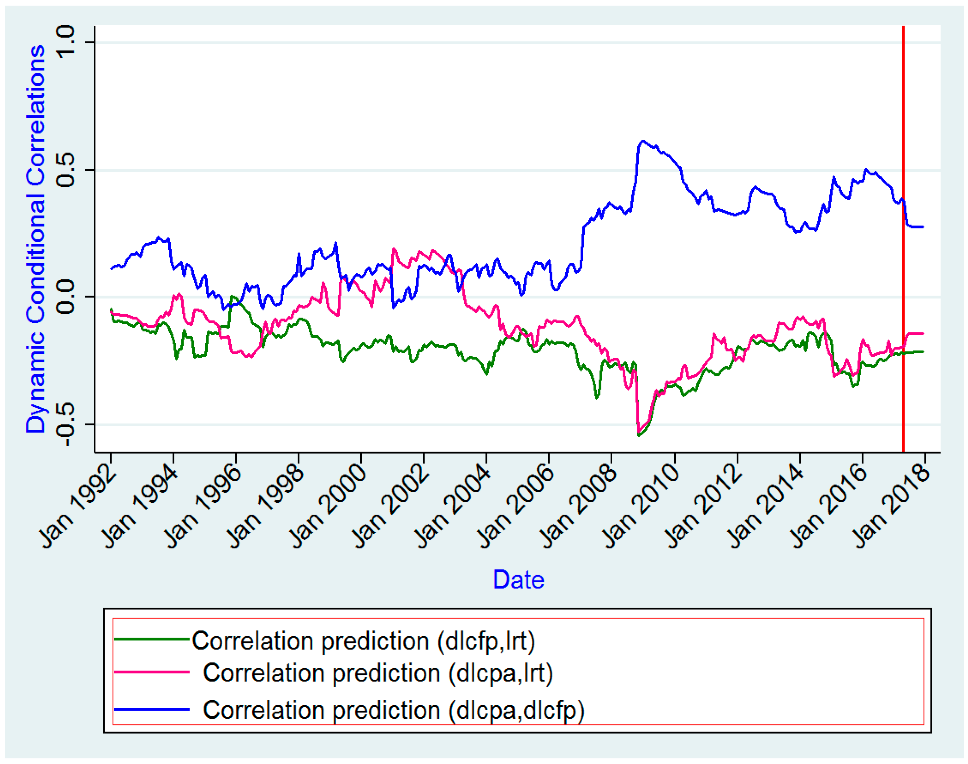
This study investigates the volatility spillovers effects of commodity price volatility, namely food and oil price volatility, on the foreign exchange market using MGARCH models. In particular, three MGARCH models are applied, including the CCC model proposed by Bollerslev (1990), which assumes that the conditional correlation is constant. However, the constant conditional correlation hypothesis of the CCC model is too restrictive, and thus may not always hold, especially in a high-frequency financial time series. As such, the study also applies the DCC model by Engle (2002), and the TCC model by Tse and Tsui (2002). The general MGARCH model is given by: $y_t=C{x}_t+{\epsilon }_t$, ${\epsilon }_t=H_t^{\frac{1}{2}}{v}_t$, where $y_t$ is an $\mathrm{m}\times 1$ vector of dependent variables; C is an $\mathrm{m}\times \mathrm{k}$ matrix of parameters; $x_t$ is a $\mathrm{k}\times 1$ vector of independent variables, which may contain lags of $y_t$; $H_t^{\frac{1}{2}}$ is the Cholesky factor of the time-varying conditional covariance matrix $H_t$; and $v_t$ is an $\mathrm{m}\times 1$ vector of zero mean, unit variance, and independent and identically distributed innovations. In the general MGARCH model, $H_t$ is a matrix generalization of univariate GARCH models. The CCC model is defined as: $H_t=D_{t}R{D}_t$, and the correlation matrix $R=\left[{\rho }_{ij}\right]$ is positive definite with ${\rho }_{ij}=1,i=1,\dots ,n.$ The off-diagonal elements of the conditional covariance matrix $H_t$ are given by: ${\left[H_t\right]}_{ij}=h_{it}^{\frac{1}{2}}{h}_{jt}^{\frac{1}{2}}{\rho }_{ij},i\ne j$. The process $\left\{a_{it}\right\}$ is modeled as a univariate GARCH. Hence, the conditional variances can be written in a vector form: $h_t=c+{\displaystyle \sum }_{j=1}^q{A}_j{a}_{t-j}^2+{\displaystyle \sum }_{j=1}^p{B}_j{h}_{t-j}$, where c is a $n\times 1$ vector, $A_j$ and $B_j$ are diagonal $n\times n$ matrices, and $a_{t-j}^2=a_{t-j}\odot a_{t-j}$ is the element-wise product. $H_t$ is ensured as positive definite when the elements of c and $A_j$ and $B_j$ are positive, since R is positive definite. The estimation of CCC models is attractive, because the correlation matrix is constant. When the correlation matric $R_t$ is time varying, $H_t$ is positive definite if $R_t$ is positive definite at each point in time and the conditional variances $h_{it},i=1,\dots ,n$ are well defined. Both the DCC and the TCC models extend the CCC model with a few extra parameters. Unlike the CCC model, time-varying model variations require that the correlation matrix be inverted for each time t in every iteration.

Several specifications of $R_t$ have been suggested in the literature. In the TCC model, GARCH-type dynamics are imposed on the conditional correlations, so that they are a function of past conditional correlations and a set of estimated correlations. More specifically, $R_t=\left(1-a-b\right)S+a{S}_{t-1}+b{R}_{t-1}$, where S is a constant, positive definite parameter matrix with ones on the diagonal, ${\theta }_1$ and ${\theta }_2$ are non-negative scalar parameters such that ${\theta }_1+{\theta }_2\le 1$, and $S_{t-1}$ is a sample correlations matrix of past M standardized residuals ${\widehat{\epsilon }}_{t-1},\dots ,{\widehat{\epsilon }}_{t-M}$, where ${\widehat{\epsilon }}_{t-j}={\widehat{D}}_{t-j}^{-1}{r}_{t-j,}j=1,\dots ,M$. The positive definiteness of $R_t$ is ensured by construction if $R_0$ and $S_{t-1}$ are positive definite. A necessary condition for this to hold is $M\ge N$. In the DCC model, the conditional correlation structure is similar to that of the TCC model in that it considers a dynamic matrix process $Q_t=\left(1-a-b\right)S+a{\epsilon }_{t-1}{\epsilon }_{t-1}^{\prime }+b{Q}_{t-1}$, where a is positive and b a non-negative scalar parameter such that $a+b<1$, S is the unconditional correlation matrix of the standardized errors ${\epsilon }_t$, and $Q_0$ is positive definite. This process ensures positive definiteness, but does not generally produce valid correlation matrices. They are obtained by rescaling $Q_t$ as follows: $R_t={\left(I\odot Q_t\right)}^{-\frac{1}{2}}{Q}_t{\left(I\odot Q_t\right)}^{-\frac{1}{2}}$. In the TCC and DCC models, the dynamic structure of the time-varying correlations is a function of past returns. The bivariate dynamic conditional correlation coefficient of Engle (2002) is, thus, defined as:

$${\mathsf{\rho }}_{12,\mathrm{t}}=\frac{{\overline{\overline{\mathrm{q}}}}_{12}\left(1-\mathrm{a}-\mathrm{b}\right)+\mathrm{a}\left({\mathsf{\epsilon }}_{1,\mathrm{t}-1}{\mathsf{\epsilon }}_{2,\mathrm{t}-1}\right)+{\mathrm{bq}}_{12,\mathrm{t}-1}}{\sqrt{\left({\overline{\overline{\mathrm{q}}}}_{11}\left(1-\mathrm{a}-\mathrm{b}\right)+{\mathrm{a}\mathsf{\epsilon }}_{11,\mathrm{t}-1}^2+{\mathrm{bq}}_{11,\mathrm{t}-1}\right)}\left(\overline{{\mathrm{q}}_{22}\left(1-\mathrm{a}-\mathrm{b}\right)+{\mathrm{a}\mathsf{\epsilon }}_{22,\mathrm{t}-1}^2+{\mathrm{bq}}_{22,\mathrm{t}-1}}\right)}$$

In the bivariate case, the conditional correlation coefficient of Tse and Tsui (2002) is defined as: ${\mathsf{\rho }}_{12,\mathrm{t}}=\left(1-{\mathsf{\theta }}_1-{\mathsf{\theta }}_3\right){\mathsf{\rho }}_{12,\mathrm{t}-1}+{\mathsf{\theta }}_3\frac{{{\displaystyle \sum }}_{\mathrm{s}=1}^{\mathrm{S}}{\mathsf{\epsilon }}_{1,\mathrm{t}-\mathrm{s}}{\mathsf{\epsilon }}_{2,\mathrm{t}-\mathrm{s}}}{\sqrt{\left({{\displaystyle \sum }}_{\mathrm{s}=1}^{\mathrm{S}}{\mathsf{\epsilon }}_{1,\mathrm{t}-\mathrm{s}}^2\right)\left({{\displaystyle \sum }}_{\mathrm{s}=1}^{\mathrm{S}}{\mathsf{\epsilon }}_{2,\mathrm{t}-\mathrm{s}}^2\right)}}$.

The study also applies the approach proposed by Diebold and Yilmaz (2012) to measure total and directional volatility spillovers. In contrast with Diebold and Yilmaz (2009), which relies on Cholesky factorization, the approach by Diebold and Yilmaz (2012) yields results that are unique and invariant to the ordering of variables. The procedure is based on the generalized VAR framework of Koop et al. (1996) and Pesaran and Shin (1998), and calculates the forecast error variance decomposition without the orthogonalization of shocks. Nevertheless, the Generalized forecast error Variance Decomposition GVD requires normality of the shock distribution, and as such, we take logarithms to make the data more normal-like. In general, for variance decompositions, own variance shares are defined to be the fractions of the $\mathrm{H}$-step-ahead error variances in forecasting $\mathrm{Yit}$ due to shocks to $\mathrm{i}$, for $\mathrm{i}=1,\dots ,\mathrm{N}$, and spillovers to be the fractions of the $\mathrm{H}$-step-ahead error in forecasting $\mathrm{Yit}$ due to shocks to $\mathrm{j}$, for $\mathrm{j}=1,2,\dots ,\mathrm{N}$, such that $\mathrm{i}\ne \mathrm{j}$. The H-step-ahead generalized variance decomposition matrix ${\mathrm{D}}^{\mathrm{gH}}=\left[{\mathrm{d}}_{\mathrm{ij}}^{\mathrm{gH}}\right]$, $\mathrm{i},\mathrm{j}=1,\dots ,\mathrm{N}$ is defined to have entries:

$${\mathrm{d}}_{\mathrm{ij}}^{\mathrm{gH}}=\frac{{\mathsf{\sigma }}_{\mathrm{ij}}{{\displaystyle \sum }}_{\mathrm{h}=0}^{\mathrm{H}-1}{\left({\mathrm{e}}_{\mathrm{i}}^{\mathrm{T}}{\mathsf{\Phi }}_{\mathrm{h}}{{\displaystyle \sum }}_{\mathrm{u}}{\mathrm{e}}_{\mathrm{j}}\right)}^2}{{{\displaystyle \sum }}_{\mathrm{h}=0}^{\mathrm{H}-1}\left({\mathrm{e}}_{\mathrm{i}}^{\mathrm{T}}{\mathsf{\Phi }}_{\mathrm{h}}{\sum }_{\mathrm{u}}{\mathsf{\Phi }}_{\mathrm{h}}^{\mathrm{T}}{\mathrm{e}}_{\mathrm{i}}\right)}·100$$

where ${\mathrm{e}}_{\mathrm{j}}$ is a selection vector with $\mathrm{j}$-th element unity and zeros elsewhere, ${\mathsf{\Phi }}_{\mathrm{h}}$ is the $\mathrm{h}$-th moving average coefficient matrix, ${\sum }_{\mathrm{u}}$ is the covariance matrix off the error terms, and ${\mathsf{\sigma }}_{\mathrm{ij}}$ is the $\mathrm{j}$-th diagonal element of ${\sum }_{\mathrm{u}}$. The denominator is the forecast error variance of variable $\mathrm{i}$, and the numerator is the contribution of shocks in variable $\mathrm{j}$ to the $\mathrm{H}$-step-ahead forcast error variance of variable $\mathrm{i}$. Given that the shocks do not need to be orthogonal, forecast error variation contributions do not necessarily sum up to 100, i.e., row sums of ${\mathrm{D}}^{\mathrm{gH}}$ are not necessarily equal to 100. Hence, in order to be able to interpret the entries of a variance decomposition matrix as shares, they have to be scaled. Hence, we use ${\tilde{\mathrm{D}}}^{\mathrm{gH}}=\left[{\tilde{\mathrm{d}}}_{\mathrm{ij}}^{\mathrm{gH}}\right]$ with $\left[{\tilde{\mathrm{d}}}_{\mathrm{ij}}^{\mathrm{gH}}\right]=\frac{\left[{\mathrm{d}}_{\mathrm{ij}}^{\mathrm{gH}}\right]}{{{\displaystyle \sum }}_{\mathrm{j}=1}^{\mathrm{N}}{\mathrm{d}}_{\mathrm{ij}}^{\mathrm{gH}}}$ instead of ${\mathrm{D}}^{\mathrm{gH}}$. The entries of ${\tilde{\mathrm{D}}}^{\mathrm{gH}}$ can be used to analyze the connectedness between assets $\mathrm{i}$ and $\mathrm{j}$. More precisely, as described in Diebold and Yılmaz (2014), the matrix ${\tilde{\mathrm{D}}}^{\mathrm{gH}}$ leads to a spillover table, which displays pairwise as well as system-wide spillovers. For a system with N variables $\left({\mathrm{Y}}_{1\mathrm{t}},\dots ,{\mathrm{Y}}_{\mathrm{Nt}}\right)$, its upper-left $\mathrm{N}\times \mathrm{N}$-block matrix contains the scaled generalized variance decomposition matrix of the $\mathrm{H}$-step-ahead forecast error, i.e.$,{\tilde{\mathrm{D}}}^{\mathrm{gH}}$. Its rightmost column contains row sums “From Others”, and the next to last bottom row contains column sums “To Others”, and the lower-right element contains the average of the column sums, where, in all of the cases, $\mathrm{i}\ne \mathrm{j}$, i.e., the diagonal elements are excluded. 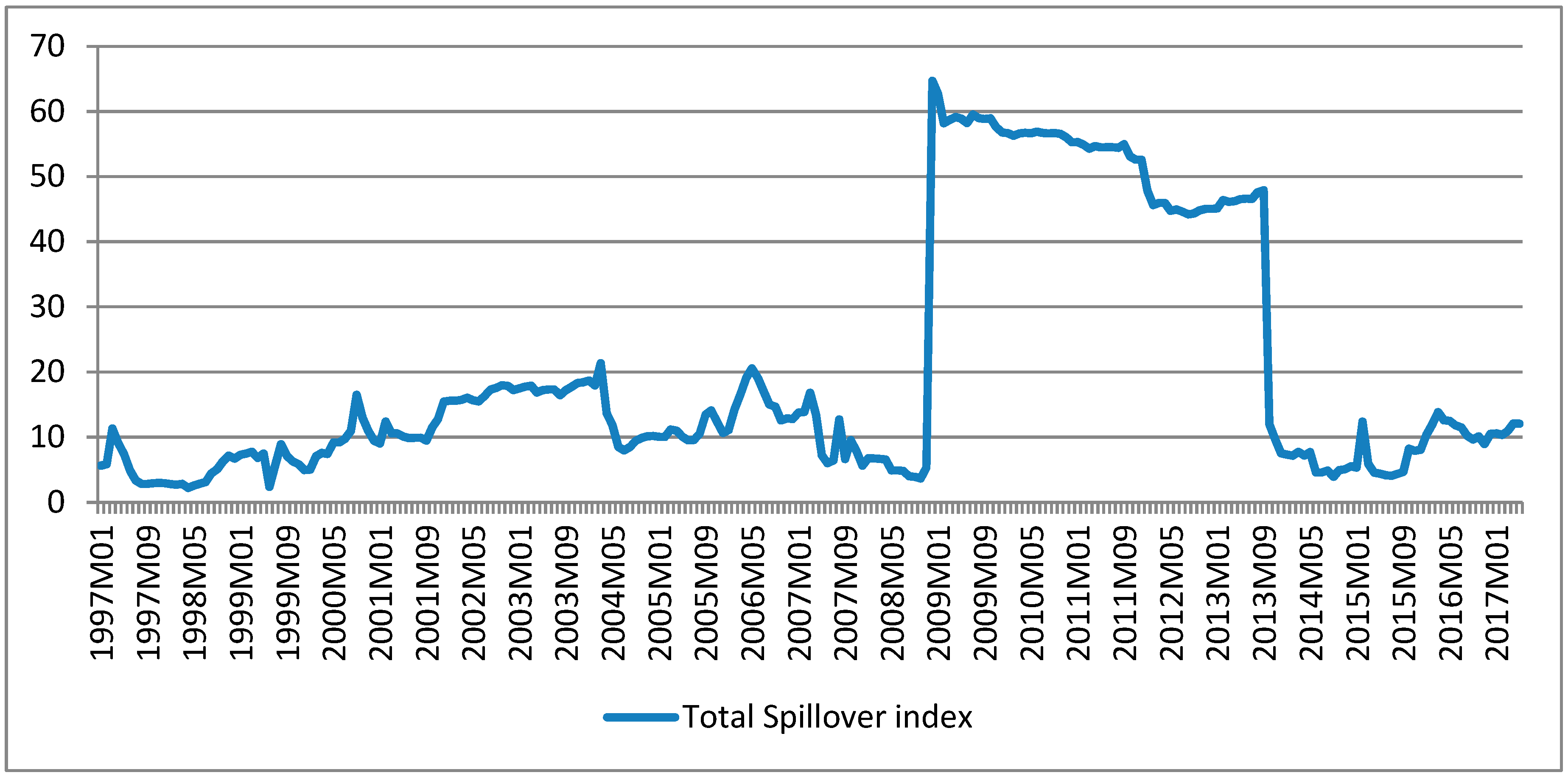The off-diagonal entries of ${\tilde{\mathrm{D}}}^{\mathrm{gH}}$ measure pairwise directional spillovers from $\mathrm{j}$ to $\mathrm{i}$. Moreover, total spillover variation over time is also assessed using a rolling window methodology that captures the evolution of the total spillover index, which is a measure of the contribution of spillovers of shocks across all variables to the total forecast error variance over time.

5. Results and Discussion

5.1. Data and Descriptive Statistics

Data on the variables of interest, namely the food price index, and crude oil price index, were obtained from the Food and Agriculture Organization and the World Bank databases respectively, while the data on the nominal exchange rate was obtained from Bank of Uganda’s database. The study focuses on the UGX/USD exchange rate mainly because it accounts for a majority of foreign currency transactions in the Ugandan economy, while the use of the food price index and crude oil price index is motivated by the strong influence of the external economic environment on Uganda’s economic performance, given her integration into the global economy. As Uganda is an oil importer and agricultural commodity exporter, volatilities of global oil and agricultural commodity prices have the potential to affect domestic consumer and investor confidence and curtail growth in the Ugandan economy.

The study uses logarithmic transformations of monthly data, in that the returns for any series analyzed in the study are defined as ${\mathrm{y}}_{\mathrm{t}}=\left({\mathrm{lnp}}_{\mathrm{t}}-{\mathrm{lnp}}_{\mathrm{t}-1}\right)$, where Pt is the price of the index series or exchange rate at time t. Preliminary evidence on the movement of prices as presented in Figure 1 below shows that the returns for all of the series tend to fluctuate around zero, and are characterized by a high degree of variability and volatility clustering, with large changes being likely to be followed by further large changes, which indicates the volatile nature of these markets. All of the returns demonstrate higher volatility around 2008, pointing to possible spillover effects.

Table 1. Summary Statistics.

	DLCFP	DLCPA	LRT
Mean	0.000	0.004	0.005
Maximum	0.070	0.203	0.163
Minimum	−0.129	−0.316	−0.083
Std. Dev.	0.026	0.082	0.025
Skewness	−0.531	−0.787	0.916
Kurtosis	5.422	4.499	9.957
Jarque-Bera	88.573 [0.000]	59.864 [0.000]	655.669 [0.000]
N	304.000	304.000	304.000
Returns correlations
Ljung–Box (2)	33.239 [0.000]	23.369 [0.000]	29.326 [0.000]
Ljung–Box (6)	41.665 [0.000]	27.225 [0.000]	30.063 [0.000]
Ljung–Box (12)	44.634 [0.000]	40.666 [0.000]	35.145 [0.000]
Tests for stationarity
ADF test	−13.130 [0.000]	−13.305 [0.000]	−13.147 [0.000]
PP Test	−13.306 [0.000]	−13.341 [0.000]	−13.120 [0.000]
KPSS Test	0.076	0.096	0.061
Test critical values:	ADF	PP	KPSS
1% level	−3.452	−3.452	0.739
5% level	−2.871	−2.871	0.463
10% level	−2.572	−2.572	0.347

Notes: LRT, DLCPA and DLCFP denote the Ugandan foreign exchange rate return volatility, food price index volatility, and crude oil price index volatility, respectively. N denotes the number of observations. p-values are in square brackets. The Jarque–Bera tests indicate the normality distribution of return series. Ljung–Box (p) is the statistic of the Ljung–Box Q-test, which tests the joint hypothesis that all of the autocorrelations are significantly different from zero. ADF: augmented Dickey–Fuller, PP: Phillip–Perron, KPSS: Kwiatkowski, Phillips, Schmidt, and Shin.

below provides a summary of descriptive statistics for the log-differenced prices of the variables of interest over the period under study. The sample period considered runs from January 1992 to April 2017, resulting in 304 observations. The choice of the sample period and data frequency is guided by data availability. The full set of statistics for the distribution of returns presented in Table 1 includes normality, correlation, and unit root tests. A look at the distributional properties of data suggests that all of the series strongly differ from the standard normal.

The descriptive statistics presented in Table 1 reveal that the unconditional distributions of the returns are skewed, besides displaying a considerable excess of kurtosis. Based on the Jarque–Bera test, the normality assumption is rejected for all three return series as well. This last feature is especially strong in the Ugandan foreign exchange market. In light of this, all of the estimations assumed a multivariate Student-t distribution. Table 1 also reports the result of Box–Pierce Q-Statistics, which tested the joint hypothesis that all the individual autocorrelation coefficients are simultaneously equal to zero for various lags. The test results reject the null hypothesis of no serial autocorrelation at examined lags for all the return series in view of the reported zero Q-statistic probabilities. The results of unit root tests carried out to inform the specification of the models applied in analyses are also presented in Table 1. The augmented Dickey–Fuller (ADF) test (Dickey and Fuller 1979), Phillip–Perron (PP) (Phillips and Perron 1988), and Kwiatkowski, Phillips, Schmidt, and Shin (KPSS) (Kwiatkowski et al. 1992) tests indicate that all of the returns series were found to be stationary.

5.2. Discussion of Results

5.2.1. Multivariate GARCH Analysis

In this section, we discuss the empirical results and analysis of our study presented in

Table 2. Estimated coefficients for conditional correlations of CCC, DCC, and VCC models.

	CCC		DCC		VCC
	Coefficient	p-Value	Coefficient	p-Value	Coefficient	p-Value
Panel A—GARCH Results
ω Exchange_rate_return	0.000 ***	0.001	0.000 ***	0.001	0.000 ***	0.001
α Exchange_rate_return	0.460 ***	0.000	0.468 ***	0.000	0.468 ***	0.000
β Exchange_rate_return	0.423 ***	0.000	0.431 ***	0.000	0.431 ***	0.000
ω Food_price_index	0.000	0.126	0.000	0.137	0.000	0.137
α Food_price_index	0.088 **	0.030	0.093 **	0.014	0.093 **	0.014
β Food_price_index	0.864 ***	0.000	0.871 ***	0.000	0.871 ***	0.000
ω Crude_oil_price_index	0.001	0.184	0.001	0.152	0.001	0.152
α Crude_oil_price_index	0.191 ***	0.009	0.182 ***	0.004	0.182 ***	0.004
β Crude_oil_price_index	0.703 ***	0.000	0.734 ***	0.000	0.734 ***	0.000
Panel B—Conditional correlation results
ρ(Exchange_rate_return, Food_price_index)	−0.209 ***	0.000	−0.134	0.321	−0.183 **	0.046
ρ(Exchange_rate_return, Crude_oil_price_index)	−0.093	0.132	−0.081	0.583	−0.069	0.469
ρ(Food_price_index, Crude_oil_price_index)	0.175 ***	0.005	0.279 *	0.091	0.242 **	0.024
Panel C—Diagnostics
df	7.867	0.000	8.176	0.000	8.184	0.000
θ1			0.034	0.050	0.046	0.163
θ2			0.931	0.000	0.873	0.000
Log-likelihood	1816		1821		1820
Wald test			1973.74	0.000	359.5	0.000
AIC	4800		4793		4796
BIC	4860		4860		4863

Note: This table provides the estimated coefficients, standard errors and p-values for the conditional correlations for the CCC—constant conditional correlation, DCC—dynamic conditional correlation, and VCC—time-varying conditional correlation multivariate generalized autoregressive conditional heteroskedasticity (MGARCH) models. ω, α, and β are estimates of the univariate GARCH(1,1) model for all three markets; conditional correlation, ρij is the correlation between market i and market j, df is the degrees of freedom, the constant correlation assumption is tested using the Likelihood Ratio test (LR Test), LR Test: θ₁ = θ₂ = 0; AIC and BIC are the Akaike Information Criterion and Schwartz Criteria, respectively. The model that yields the lowest AIC (BIC) value is considered to generate the data best. Using AIC and BIC, the CCC model has slightly smaller AIC and BIC values, and thus is the preferred model according to these criteria. The asterisks ***, **, and * represent 1%, 5%, and 10% significance level, respectively.

below. The results for the estimated CCC (1,1), DCC(1,1), and VCC(1,1) models are comparatively similar. Panel A reports the parameter estimates for the conditional variance models of each market, where ω is the estimated constant term for each conditional variance, and α and β represent the estimated own autoregressive conditional heteroskedasticity (ARCH) and GARCH parameters, respectively. The estimated α and β parameters for each market are significantly different from zero, suggesting the existence of individualized ARCH and GARCH effects. The CCC, DCC, and varying conditional correlation (VCC) models all reveal volatility persistence as the sum of the calculated parameters for very close to unity for both the results of the univariate GARCH estimations.

Panel B of the table reports the corresponding conditional correlations between various pairs of markets. In all of the estimated models, all of the estimated conditional correlations are significantly different from zero at the 1% significance level, with the exception of the conditional correlations between the Ugandan foreign exchange rate return volatility and the volatility of crude oil price index returns. The level of conditional correlations between markets is relatively low in all of the estimated models. For example, with respect to the CCC model, the conditional correlation between the exchange rate return volatility and food price index volatility is −0.209, while the conditional correlation between the food price index volatility and crude oil price index volatility is 0.175. Thus, the study finds evidence of weak volatility spillover effects from the commodity market through the food price index volatility to the Ugandan foreign exchange rate market, and also weak spillover effects for the food price index to the crude oil price index commodity markets. The low conditional correlation between the exchange rate return volatility and food price index volatility reflects the low interconnectivity between these markets, implying that factors other than food price index volatility explain the patterns of excess volatility in the Ugandan foreign exchange market.

The statistically significant negative coefficient on the conditional correlation between exchange rate volatility and food price index volatility in all of the models suggests that an increase in food price index volatility is associated with a somewhat decreased volatility of the Ugandan exchange rate. This may be due to the exchange rate appreciation gains resulting from a positive commodity price shock for the Ugandan economy, which is still heavily dependent on primary agricultural commodity exports. Consistent with the extant literature, the estimated constant conditional correlation between food price index volatility and crude oil price index volatility is positive, suggesting that both markets are exposed to common shocks. However, the small estimated coefficient for all of the models reflects the lower co-movements between the two markets. Low but statistically insignificant conditional correlations occur between the Ugandan foreign exchange rate return volatility and the volatility of crude oil price index returns in all of the estimated models.

The diagnostics for estimated models are reported in Panel C. The results show evidence of time-varying conditional correlations in both the DCC and VCC models, supporting evidence in the literature that suggests that the assumption of constant conditional correlation for all shocks to return is not supported empirically. Nevertheless, only the DCC model has positive and statistically significant estimated coefficient parameters for θ₁ and θ₂ at the 10% level. The estimated parameters for θ₁ and θ₂ sum to a value close to one, implying that volatility exhibits a highly persistent behavior. Nevertheless, since the sum is a value less than one, the dynamic conditional correlations are mean reverting. The magnitudes of parameters θ₁ and θ₂ indicate that the evolution of the conditional covariance depends more on its past values than on lagged residuals’ innovations, such that shock persistence has a greater impact in the long run (see coefficients for θ₂ in all of the models) as compared to the short-run (see coefficients for θ₁ in all of the models). In addition, only the DCC model provides statistically significant evidence for the existence of short-run volatility shock spillover effects. The significance of θ₁ and θ₂ in the DCC model suggests that conditional correlations are highly dynamic and time varying, which is an indication that the assumptions of CCC do not hold, which is consistent with evidence in the literature.

In order to further confirm the reliability of our estimation results, we carry out additional model diagnostic tests. The DCC and VCC models reduce to a CCC model when θ₁ = θ₂ = 0. In Table 2, the results for both the DCC and VCC show that their respective Wald test results reject the null hypothesis that θ₁ = θ₂ = 0 at all of the conventional significance levels, which is an indication that the assumption of time-invariant conditional correlations maintained in the CCC model is too restrictive for the data. According to the information criterion tests in Table 1, the DCC model, which consistently has the lowest estimated coefficients for the AIC and BIC criteria, is the best model of the three MGARCH models.

Figure 2 shows the evolution of conditional correlations over the sample period based on the DCC model. It is evident from Figure 2 that the conditional correlations are not constant over time, and are especially volatile during and after the global financial crisis of 2007–2008. Figure 2 highlights the weak correlation in volatility for all of the series pairs in the period preceding the global financial crisis, suggesting that volatility spillovers were exacerbated by the global financial crisis. Moreover, it seems that the volatilities of the exchange rate and both commodity price indices have a similar pattern, moving in opposite directions, while the volatility of the food and oil price commodity indices generally moves in the same direction. Thus, the study finds evidence of volatility spillover effects based on the significant conditional correlations pointing to an increase in returns volatility co-movements over time.

5.2.2. Spillover Analysis in a Generalized VAR Framework

In

Table 3. Spillover indices for volatility using a generalized vector autoregressive framework.

	lrt	dlcpa	dlcfp	$\mathbf{ALL}\mathbf{to} \mathbf{i}$
lrt	97.68	0.61	1.71	2.32
dlcpa	9.99	89.35	0.66	10.65
dlcfp	8.01	15.20	76.79	23.21
$\mathrm{i}$ to ALL	18.00	15.81	2.37	12.06
Net $\mathrm{i}$ to ALL	15.68	5.16	−20.84	0.00

Notes: lrt, dlcpa, and dlcfp denote the Ugandan foreign exchange rate return volatility, food price index volatility, and crude oil price index volatility, respectively.

, spillover indices among the considered variables are presented. The directional spillover indices, ALL to i, i to ALL, and Net i to ALL, describe the spillovers received by market i from all of the other markets, spillovers transmitted by market i to all of the other markets, and the difference between these two measures, respectively. The remaining rows of the Table 3 comprise the gross pairwise spillover indices, showing the contribution of a market to another particular market. The results for each market show large values of the diagonal entries of the upper-left matrix (“own connectedness”) in each column, especially for the Ugandan foreign exchange rate return volatility of 97.7% suggesting that a large percentage of the forecast error variance of the Ugandan foreign exchange rate return comes from its own volatility. In addition, the total directional connectedness (“ALL to i” or “i to ALL”) is less than the “own connectedness” for all of the variables, suggesting that cross-market volatility spillovers are quite limited in these markets. This is confirmed by the low value of the total spillover index of 12.1%, which describes the portion of the forecast error variance that comes from all of the spillovers, and is an average impact of connectedness. Thus, the study finds that the finding of low market volatility spillover using the Diebold and Yilmaz (2012) approach is consistent with the findings of low market interconnectedness using the MGARCH analysis.

Next, we look at the pairwise directional connectedness of the largest value of the pairwise directional connectedness from crude oil price index volatility to food price index volatility of 15.2%, followed by the exchange rate volatility to crude oil price index volatility of 10.0%. From the Net $\mathrm{i}$ to ALL rows, the exchange rate volatility is identified as the main contributor of volatility to the other markets, even though the magnitude of the associated volatility spillover is low. This may be justified by the high volatility of the Uganda shilling and US dollar exchange rate during the analysis period, leading oil investors to become more sensitive to an increase of volatility in the exchange rate. In addition, the pairwise directional connectedness of the exchange rate volatility to food price index volatility is of a fairly similar magnitude of 8.0%, which is an indication that the exchange rate and commodity markets are volatile for domestic currencies against the US dollar whose trade relies extensively on dollar invoicing. Thus, this a key factor of commodity price volatility. Nevertheless, the low level of the volatility transmission suggests a low level of connectivity between the Ugandan exchange rate market and the commodity price markets considered in this analysis. The “ALL to $\mathrm{i}$” connectedness measures range from 2.3% to 23.2% while the “to” connectedness measure ranges between 2.4% to 18.0%. The net total directional connectedness measure is negative only for the case of food price index volatility, which is an indication that this variable is a net receiver of volatility, while exchange rate volatility and crude oil price index volatility are net transmitters of volatility, even though the magnitudes are relatively low.

The study further estimates the total volatility spillover index by applying 60-month rolling samples that enable us to capture the evolution of volatility spillovers over time. As may be seen in Figure 3, volatility spillovers vary over time. The total volatility spillover index started by fluctuating around 10%, although this pattern is considerably violated during the periods corresponding to the collapse of Lehman Brothers in September 2008 and the subsequent global financial crisis, as well as the 2011 debt crisis in Europe. The intensity of volatility spillovers averaged at 52.8% of the forecast error variance during crisis periods. Thus, the time-varying behavior of the total spillover index reveals an intensification of volatility spillovers during periods of high uncertainty, especially during the global financial crisis period and sovereign debt crisis in Europe. It is in this period that volatility spillovers reached their highest values.

5.3. Sensitivity and Robustness Analysis

The use of GARCH-type models is premised on the presence of ARCH effects. The ARCH LM test is a test of the null hypothesis of no ARCH effects up to order q in the residuals. Thus, before estimating the three MGARCH models, the study carried out a test for the presence of ARCH effects using the ARCH LM test and Breusch–Pagan test. Based on the p-values for the ARCH LM and Breusch–Pagan test of 0.02 and 0.001 respectively, we reject the null hypothesis of homoscedasticity at the 5% significance level, and conclude that there is a presence of heteroskedasticity and consequently proceeded with the estimation of the various MGARCH models.

In order to enrich the analysis, we checked for model sensitivity by analyzing three different variations of conditional variance models that have been used to analyze spillover effects in the literature. A comparative table summarizing the statistical performance of each approach is presented in Table 2. The results for both models are qualitatively similar, with comparable magnitudes and signs of the coefficients. The multivariate Student-t distribution was represented with the degrees of freedom (df) as an extra parameter that indicates the number of statistical moments in the multivariate distribution. Since the estimated df parameters in all of the models exceeded the value of four, evidently, fourth-order moments exist.

We also checked the robustness of the volatility spillover analysis by comparing the results of the generalized variance decomposition proposed by Diebold and Yilmaz (2012) with the Cholesky factorization approach of Diebold and Yilmaz (2009).1 Since the results of the Cholesky factorization approach crucially depend on the ordering of the variables, it is not suitable for assessing pairwise and total directional connectedness, but it should be robust for total connectedness. The results of the total volatility spillover measure for the generalized variance decomposition approach and the Cholesky factorization are quite similar. In addition, the results of the total spillover index based on the generalized variance decomposition for VAR (p) with p = 3, 4 and W = 60,120 are fairly similar.

5.4. Limitation and Suggestions for Future Research

The results discussed above are based on a very short time span and low-frequency data, which may present challenges in conducting a more comprehensive analysis of the time-varying spillover effects in the data.

6. Conclusions and Recommendations

The objective of this paper was to empirically investigate the spillover effects, if any, of oil and food price volatility on the volatility of a key macroeconomic indicator of importance to financial stability in Uganda: the nominal Uganda shilling per United States dollar (UGX/USD) exchange rate. The study applies various MGARCH models, including the CCC, DCC, and VCC and the GVAR framework proposed by Diebold and Yilmaz (2012), and finds that in line with the extant literature, cross-market interconnectedness and volatility spillovers were quite limited until the onset of the global financial crisis, as evidenced by the weak dynamic conditional correlations in returns, as well as the low value of the total spillover index. The analyses of time-varying dynamic conditional correlations and total spillover index also reveal an intensification of market interconnectedness and sharp increases volatility spillovers during periods of high uncertainty and market crises, particularly during the global financial crisis and sovereign debt crisis periods. Thus, the evidence points to the existence of significant spillover effects in the Ugandan foreign exchange market during crisis periods. The ongoing study of spillover effects between markets is important for policy makers as well as market participants, as their impact varies through time. In order to address the excessive volatility spillovers during crisis periods, Uganda as a commodity-dependent economy can adopt revenue stabilization funds not only for ensuring macroeconomic stability and intergenerational equity, but also to minimize exchange rate volatility. The findings of the study may also inform the activity of the central bank of Uganda in the foreign exchange rate market, which is aimed at influencing the exchange rate in a manner that will support financial sector stability, especially during crisis periods. However, in the long run, diversification and industrialization remain the best means for the country to reduce its external and internal vulnerability, as well as effectively deal with the adverse effects of economic crises.

References

1. Alghalith, Moawia. 2010. The Interaction between Food Prices and Oil Prices. Energy Economics 32: 1520–22. [Google Scholar] [CrossRef]
2. Bank of Uganda. 1999. Bank of Uganda Annual Report 1998/99. Kampala: Bank of Uganda. [Google Scholar]
3. Bank of Uganda. 2009. Bank of Uganda Annual Report 2008/09. Kampala: Bank of Uganda. [Google Scholar]
4. Bank of Uganda. 2011. Bank of Uganda Annual Report 2010/11. Kampala: Bank of Uganda. [Google Scholar]
5. Bank of Uganda. 2016. About the Bank. Available online: https://www.bou.or.ug/bou/home.html (accessed on 11 September 2018).
6. Baruník, Jozef, Evžen Kočenda, and Lukáš Vácha. 2017. Asymmetric Volatility Connectedness on the Forex Market. Journal of International Money and Finance 77: 39–56. [Google Scholar] [CrossRef]
7. Becketti, Sean, and Gordon H. Sellon Jr. 1989. Has Financial Market Volatility Increased? Economic Review-Federal Reserve Bank of Kansas City 74: 17. [Google Scholar]
8. Bollerslev, Tim. 1990. Modelling the Coherence in Short-Run Nominal Exchange Rates: A Multivariate Generalized ARCH Model. The Review of Economics and Statistics, 498–505. [Google Scholar] [CrossRef]
9. Bouri, Elie, and Riza Demirer. 2016. On the Volatility Transmission between Oil and Stock Markets: A Comparison of Emerging Importers and Exporters. Economia Politica 33: 63–82. [Google Scholar] [CrossRef]
10. Chen, Sheng-Tung, Hsiao-I Kuo, and Chi-Chung Chen. 2010. Modeling the Relationship between the Oil Price and Global Food Prices. Applied Energy 87: 2517–25. [Google Scholar] [CrossRef]
11. Creti, Anna, Marc Joëts, and Valérie Mignon. 2013. On the Links between Stock and Commodity Markets’ Volatility. Energy Economics 37: 16–28. [Google Scholar] [CrossRef]
12. Crockett, Andrew. 1996. The Theory and Practice of Financial Stability. De Economist 144: 531–68. [Google Scholar] [CrossRef]
13. Dickey, David A., and Wayne A. Fuller. 1979. Distribution of the Estimators for Autoregressive Time Series with a Unit Root. Journal of the American Statistical Association 74: 427–31. [Google Scholar]
14. Diebold, Francis X., and Kamil Yilmaz. 2009. Measuring Financial Asset Return And Volatility Spillovers, with Application To Global Equity Markets. The Economic Journal 119: 158–71. [Google Scholar] [CrossRef]
15. Diebold, Francis X., and Kamil Yilmaz. 2012. Better to Give than to Receive: Predictive Directional Measurement of Volatility Spillovers. International Journal of Forecasting 28: 57–66. [Google Scholar] [CrossRef]
16. Diebold, Francis X., and Kamil Yılmaz. 2014. On the Network Topology of Variance Decompositions: Measuring the Connectedness of Financial Firms. Journal of Econometrics 182: 119–34. [Google Scholar] [CrossRef]
17. Engle, Robert. 2002. Dynamic Conditional Correlation: A Simple Class of Multivariate Generalized Autoregressive Conditional Heteroskedasticity Models. Journal of Business & Economic Statistics 20: 339–50. [Google Scholar]
18. Engle, Robert F., Takatoshi Ito, and Wen-Ling Lin. 1990. Meteor Showers or Heat Waves? Heteroskedastic Intra-Daily Volatility in the Foreign Exchange Market. Econometrica 58: 525–42. [Google Scholar] [CrossRef]
19. Ghosh, Saurabh. 2014. Volatility Spillover in the Foreign Exchange Market: The Indian Experience. Macroeconomics and Finance in Emerging Market Economies 7: 175–94. [Google Scholar] [CrossRef]
20. Henstridge, Mark, and Louis Kasekende. 2001. Exchange Reforms, Stabilization and Fiscal Management. In Uganda’s Recovery–The Role of Farms, Firms, and Government. Edited by Ritva Reinikka and Paul Collier. Washington, DC: The World Bank, pp. 49–80. [Google Scholar]
21. IMF. 2003. Fund Assistance for Countries Facing Exogenous Shocks. Policy papers. Washington, DC, USA: International Monetary Fund. [Google Scholar]
22. Jacks, David S., Kevin H. O’Rourke, and Jeffrey G. Williamson. 2010. Commodity Price Volatility and World Market Integration since 1700. The Review of Economics and Statistics 93: 800–13. [Google Scholar] [CrossRef]
23. Jondeau, E., S. H. Poon, and M. Rockinger. 2007. Financial Modeling Under Non-Gaussian Distributions. Illustrate. Springer Finance. London: Springer Science & Business Media. [Google Scholar]
24. Kasekende, L. A., M. Atingi-Ego, and R. K. Sebudde. 2004. The African Growth Experience Uganda Country Case Study Growth Working Papers. Growth Working Papers. [Google Scholar]
25. Koop, Gary, M. Hashem Pesaran, and Simon M. Potter. 1996. Impulse Response Analysis in Nonlinear Multivariate Models. Journal of Econometrics 74: 119–47. [Google Scholar] [CrossRef]
26. Kumar, Dilip. 2017. On Volatility Transmission from Crude Oil to Agricultural Commodities. Theoretical Economics Letters 7: 87–101. [Google Scholar] [CrossRef]
27. Kwiatkowski, Denis, Peter C. B. Phillips, Peter Schmidt, and Yongcheol Shin. 1992. Testing the Null Hypothesis of Stationarity against the Alternative of a Unit Root: How Sure Are We That Economic Time Series Have a Unit Root? Journal of Econometrics 54: 159–78. [Google Scholar] [CrossRef]
28. Lin, Xiaowen Sharon, and Michael N. Tamvakis. 2001. Spillover Effects in Energy Futures Markets. Energy Economics 23: 43–56. [Google Scholar] [CrossRef]
29. Milunovich, George, and Susan Thorp. 2006. Valuing Volatility Spillovers. Global Finance Journal 17: 1–22. [Google Scholar] [CrossRef]
30. Mo, Bin, He Nie, and Yonghong Jiang. 2018. Dynamic Linkages among the Gold Market, US Dollar and Crude Oil Market. Physica A: Statistical Mechanics and Its Applications 491: 984–94. [Google Scholar] [CrossRef]
31. Mugume, Adam. 2008. Market Structure and Performance in Uganda’s Banking Industry. Unpublished Working Paper. [Google Scholar]
32. Pesaran, H. Hashem, and Yongcheol Shin. 1998. Generalized Impulse Response Analysis in Linear Multivariate Models. Economics Letters 58: 17–29. [Google Scholar] [CrossRef]
33. Phillips, Peter C. B., and Pierre Perron. 1988. Testing for a Unit Root in Time Series Regression. Biometrika 75: 335–46. [Google Scholar] [CrossRef]
34. Raddatz, Claudio. 2007. Are External Shocks Responsible for the Instability of Output in Low-Income Countries? Journal of Development Economics 84: 155–87. [Google Scholar] [CrossRef]
35. Reszat, Beate. 2002. The Japanese Foreign Exchange Market. London: Routledge. [Google Scholar]
36. Rickne, Johanna. 2009. Oil Prices and Real Exchange Rate Movements in Oil-Exporting Countries: The Role of Institutions. Stockholm: Research Institute of Industrial Economics. [Google Scholar]
37. Sadorsky, Perry. 2012. Correlations and Volatility Spillovers between Oil Prices and the Stock Prices of Clean Energy and Technology Companies. Energy Economics 34: 248–55. [Google Scholar] [CrossRef]
38. Sadorsky, Perry. 2014. Modeling Volatility and Correlations between Emerging Market Stock Prices and the Prices of Copper, Oil and Wheat. Energy Economics 43: 72–81. [Google Scholar] [CrossRef]
39. Samanta, Subarna K., and Ali H. M. Zadeh. 2012. Co-Movements of Oil, Gold, the US Dollar, and Stocks. Modern Economy 3: 111–17. [Google Scholar] [CrossRef]
40. Tse, Yiu K., and Albert K. C. Tsui. 2002. A Multivariate Generalized Autoregressive Conditional Heteroscedasticity Model with Time-Varying Correlations. Journal of Business & Economic Statistics 20: 351–62. [Google Scholar]
41. Tumusiime-Mutebile, Emmanuel. 2011. Bank of Uganda’s Position on the Exchange Rate. Kampala: BIS Central Bankers’ Speeches, Bank for International Settlements. [Google Scholar]
42. Tumusiime-Mutebile, Emmanuel. 2012. Macroeconomic Management in Turbulent Times. Kyankwanzi and Kampala: BIS Central Bankers’ Speeches, Bank for International Settlements. [Google Scholar]
43. UNCTAD (United Nations Conference on Trade and Development). 2012. Excessive Commodity Price Volatility: Macroeconomic Effects on Growth and Policy Options. Geneva: United Nations Conference on Trade and Development. [Google Scholar]
44. Varangis, Panos, Sona Varma, Angelique DePlaa, and Vikram Nehru. 2004. Exogenous Shocks in Low Income Countries: Economic Policy Issues and the Role of the International Community. Background Paper Prepared for the Report: Managing the Debt Risk of Exogenous Shocks in Low Income Countries. Washington, DC: The World Bank. [Google Scholar]
45. Wei, Ching-Chun, and Chung-Hsuan Chen. 2014. Does WTI Oil Price Returns Volatility Spillover to the Exchange Rate and Stock Index in the US? International Journal of Energy Economics and Policy 4: 189–97. [Google Scholar]
46. Whitworth, Alan, and Tim Williamson. 2010. Overview of Ugandan Economic Reform since 1986. In Uganda’s Economic Reforms Insider Accounts. Edited by Florence Kuteesa, Emmanuel Tumusiime-Mutebile, Alan Whitworth and Tim Williamson. New York: Oxford University Press Inc. [Google Scholar]
47. World Bank. 2015. World Development Indicators. Washington, DC: World DataBank. [Google Scholar] [CrossRef]
48. World Bank. 2016. Uganda Overview. Worldbank.org. Available online: http://www.worldbank.org/en/country/uganda/overview (accessed on 29 April 2016).
49. Zhang, Yue-Jun, Ying Fan, Hsien-Tang Tsai, and Yi-Ming Wei. 2008. Spillover Effect of US Dollar Exchange Rate on Oil Prices. Journal of Policy Modeling 30: 973–91. [Google Scholar] [CrossRef]
1
The detailed Cholesky factorization analyses are not reported in this paper, but can be requested from the author.
Figure 1. Logarithmic returns of exchange rate, food, and crude oil commodity price indices.
Economies 07 00001 g001
Figure 2. Evolution of dynamic conditional correlations. Notes: lrt, dlcpa and dlcfp denote the Ugandan foreign exchange rate return volatility, food price index volatility, and crude oil price index volatility, respectively.
Economies 07 00001 g002
Figure 3. Evolution of the total spillover index.
Economies 07 00001 g003