Downshifting in the Fast Lane: A Post-Keynesian Model of a Consumer-Led Transition

Abstract

If the world’s countries seriously tackle the climate targets agreed upon in Paris, their citizens are likely to experience substantial changes in production, consumption, and employment. We present a long-run post-Keynesian model for studying the potential implications of a major transition on macroeconomic stability and employment. It is a demand-led model in which firms have considerable but not absolute freedom to administer prices, while household consumption exhibits inertia. Firms continually seek input-saving technological improvements that, in aggregate, tie technological progress to firms’ cost structures. Together with firm pricing strategies and wage setting, the productivities of different inputs determine the functional income distribution. Saving and investment, and production and purchase of consumption goods, are undertaken by different economic actors, driven by income and capacity utilization, with the possibility that productive capacity exceeds, or falls short of, effective demand. The model produces business cycles and long waves driven by technological change. We present results for a “downshifting” scenario in which households voluntarily withdraw labor, and discuss the implications of downshifting for stability, growth, and employment. We contrast the downshifting scenario with ones in which households reduce consumption without withdrawing from the labor pool.

1. Introduction

Shifting to a low-carbon economy is vital to limiting global temperature and curbing dangerous levels of climate change. World leaders committed themselves to climate action when over 195 countries (UNFCCC 2016) signed the historic Paris Agreement and pledged to take appropriate climate mitigation actions1 to restrict global temperature increases to below 1.5 °C (UNFCCC 2015). However, proposed country actions submitted as of November 2016 are insufficient to meet the temperature limit (Climate Action Tracker 2017). Ultimately, to prevent further warming, it will be essential to keep most of the remaining fossil fuels in the ground (McGlade and Ekins 2015; Benedikter et al. 2016). Because fossil fuel consumption has underpinned human development in the last two centuries, there is great reluctance to transition to different fuels.

Given the urgency of the climate challenge, the question before us is: how can we accelerate a low-carbon transition? Recommendations tend to focus on technological choice and investment (UNEP 2011; OECD 2011; Green Growth Action Alliance 2013), yet there are reasons to think that major societal and lifestyle changes must accompany a low-carbon transition, as in all major technological transitions (Rhodes 2007; Bridge et al. 2013). If the transition is to be intentional and rapid, it raises the question of the different roles of producers and consumers in initiating change.

In this paper we focus on middle- to high-income households in high-income countries in their roles as workers and consumers. Given global constraints on human activity—planetary boundaries (Rockström et al. 2009)—and a finite carbon budget (Messner et al. 2010), equity considerations imply a need for reduced physical throughput in high-income economies. The continued close association between GDP and material and energy flows (Ayres and Warr 2010) suggests we must make quality of life depend on more than GDP (e.g., Victor 2008; Jackson 2009), allowing GDP growth to slow, and perhaps even fall, for a time in high-income countries (Kallis et al. 2012). Schor (2001) argues that reduced working hours in high-income countries, or “downshifting”, is a strategy to address the “triple imperative” of reducing pressure on the environment, global poverty, and erosion of social capital in the course of economic development.

According to Schor (2001, p. 14), downshifting is “a quiet shift in values and behaviors away from consumerism. Downshifters either withdraw or partially withdraw from the labor force, mainly in order to achieve more balance, control, and less stress in life”. It is a strategy open to comparatively wealthy households and is motivated mainly by concerns over quality of life, rather than the environment. Nevertheless, it may have environmental benefits (Kennedy et al. 2013), particularly among the households with the largest environmental footprints.

Reducing working hours means less expenditure and less output. The same effect can be achieved by simply buying less, without reducing working hours. However, as we illustrate with the model described in this paper, the effects of the two strategies are quite different. Buying less without working less means higher savings, but also less incentive for companies to invest. This results in unemployment, but not immediately, and almost certainly not for the household that first curtailed its consumption. Reducing working hours, on the other hand, combines reduced employment with reduced expenditure within the same household.

Rezai et al. (2013) pointed out that downshifting may have perverse outcomes, because withdrawing labor will tighten the labor market, thereby driving up wages and inducing labor-saving technological change. They suggest that understanding the impact of downshifting requires analysis of the economy in aggregate. In this paper we present scenarios of downshifting and reduced consumption using a model capable of addressing this question. It is being developed in order to better understand the dynamics of a transition to a low-carbon economy, and is in active development. A detailed mathematical presentation of the model, now slightly out of date, can be found in a separate paper (Kemp-Benedict 2017c). In this paper we present only the main equations.

2. Methodology

We draw on several theoretical traditions, while remaining broadly within post-Keynesian economics (Lavoie 2014). Thus, this paper is one of a growing number that apply post-Keynesian theory to ecological economics and sustainability (Guarini and Porcile 2016; Fontana and Sawyer 2016; Taylor et al. 2016; Guarini 2015). We follow ecological economics in viewing economies as open systems embedded in societies, which are embedded in nature (Costanza et al. 2012). From evolutionary economics we draw the idea that economies are normally out of equilibrium (Schumpeter 1928; Nelson and Winter 1982), and from Blatt (1983) that the average state of the economy may differ substantially from the equilibrium. Following a long tradition in economics (Knight 1921; Keynes 1936; Shackle 1949), we view the future as fundamentally uncertain: a central concept in post-Keynesian economics (Davidson 1991; Dunn 2001). Because of uncertainty, economic actors’ beliefs about the future significantly influence the trajectory of the economy (Beckert 2016). Theoretical and empirical work in post-Keynesian economics demonstrates the importance of demand, as well as supply, to long-run growth (Setterfield 2002). Moreover, demand and supply co-evolve (Witt 2001). With the Sraffians (Aspromourgos 2004), we agree that changes in the sectoral composition of production and consumption are relevant to long-term growth, and that the distribution of income between profits and wages is influenced by wider social forces. Both the evolutionary and post-Keynesian perspectives emphasize the historically contingent and path-dependent nature of economic change.

We follow a general approach to macroeconomic modeling (cf. L. Taylor 2004), in which a set of economic balances, or accounts, is supplemented by behaviors of economic actors. Once actors have acted, the accounts are typically out of balance, so some parameter or combination of parameters must adjust to clear the accounts. Once all of the accounts, behaviors, and clearing mechanisms are specified, the model is closed. Because models must be closed, fundamental uncertainty and openness pose a challenge, but they are features of the real world, and they make a low-carbon transition imaginable. We follow Setterfield (2003) by treating behaviors and clearing mechanisms as conditional, dependent on both the research question and on historically contingent features of the economy. This approach combines well with a scenario analysis (Bishop et al. 2007). To be useful, a scenario model must be flexible enough to represent different narratives while representing relevant systems sufficiently well to keep the scenarios within the wide but finite bounds of what can realistically be posited about alternative futures (Bell 1997). In the accounts-behaviors-clearing mechanisms approach to model-building, different scenarios can be distinguished by different behavioral assumptions and pathways for exogenous variables. They may also differ in the way the accounts are cleared. More rarely, the accounts themselves may change.

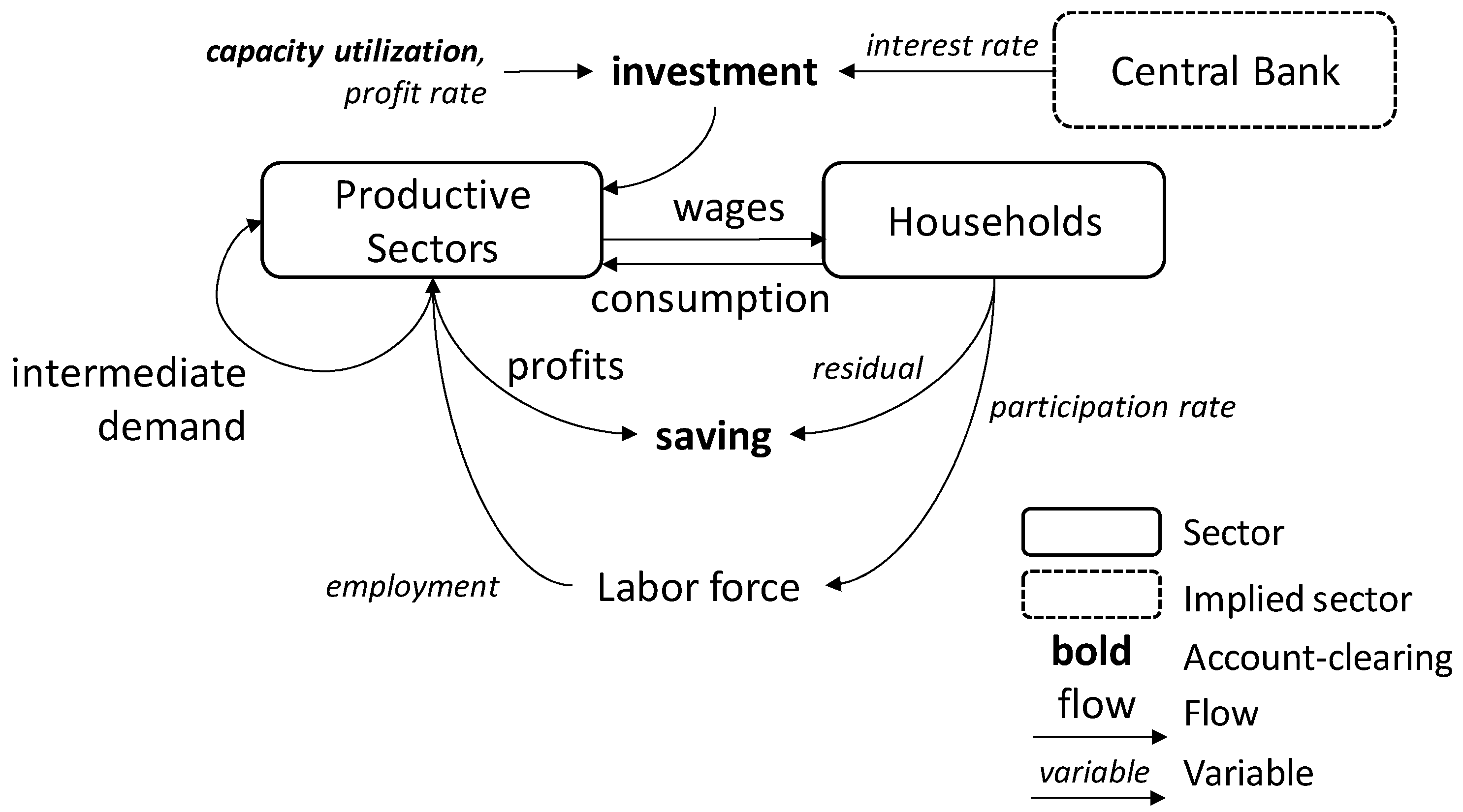
The essential components of the model documented by Kemp-Benedict (2017c) are shown in Figure 1. It has five productive sectors: services, construction, manufacturing, agriculture, and mining. It is a closed economy model with no government sector. The model is demand-led, adjusting gradually through changes in capital and labor productivity, pricing decisions of firms, wage-setting, and capital accumulation.

2.1. Saving and Investment

In keeping with post-Keynesian theory (Lavoie 2014), separate decisions govern saving and investment, so they are typically out of balance once actors have acted. The accounts are cleared by adjusting capacity utilization. Thus the model allows for underutilization of capital and unemployment. We assume that all profits are saved, so although those profits may be retained by firms or paid to households, in Figure 1 we show profits as a direct line from the productive sectors to saving. Households may also save, or borrow, in an amount determined by the gap between their wage income and their consumption.

Investment is determined by an investment function. When capital stocks are operating at relatively high capacity, it is a signal to firms that more investment is needed; conversely, when utilization is low, it is a signal to slow down investment. Investment funds come implicitly from retained profits, bank loans, or equity investment. Equity investors respond to returns. While the model has no government sector, it implicitly includes a central bank, which sets an interest rate. Higher interest rates mean higher borrowing costs, which discourages firms from taking on bank loans. The investment rate (that is, new investment divided by the value of the capital stock) is therefore an increasing function of both capacity utilization and the profit rate, and a decreasing function of the interest rate.

Following Hicks (1950), we express investment function g_i, defined separately for each sector by a subscript i, as the sum of autonomous and induced components,

$$g_i=g_i^{\mathrm{aut}}+g_i^{\mathrm{ind}}.$$

(1)

The induced component depends on utilization u_i, profit rate r_i, and the interest rate i, but also has a floor determined by the depreciation rate. On the assumption that not all firms disinvest in a downturn by allowing their stock to depreciate, the floor is set to a fraction f of the sector-specific depreciation rate δ_i,

$$g_i^{\mathrm{ind}}=\max \left[{\alpha }_i\left(u_i-u^{\ast }\right)+\beta \left(r_i-r_i^{\ast }\right)-\gamma \left(i-i^{\ast }\right),-f{\delta }_i\right].$$

(2)

In this expression, the normal utilization rate u*, target rate of return r*, and real neutral rate of interest i* are exogenous parameters. As indicated by subscripts, utilization sensitivity can vary between sectors, and each sector has a different target profit rate. Other parameters are the same across sectors.

The autonomous investment rate tracks the induced rate with a lag. The induced rate is first smoothed, using an exponential smoother, and then the lagged, smoothed, induced rate is used to update the autonomous investment rate,

$$g_i^{\mathrm{aut}}=g_{i,-1}^{\mathrm{aut}}+{\langle g_i^{\mathrm{ind}}\rangle }_{-1}.$$

(3)

In the final term, the brackets indicate an exponentially smoothed value.

2.2. Economic Growth

Growth in economic output is driven mainly by population growth and change in labor productivity. Population in the model is calculated using a three-cohort demographic model, in which the working-age population (cohort 2) has children (cohort 1), most of whom eventually grow up to join the workforce, and eventually retire (cohort 3). The model also allows for immigration into the working-age cohort and death in all three cohorts.

Labor productivity increases mainly through the use of labor-saving (and resource-using) machines, but also through improved use of existing machines. Thus, labor productivity can follow either from technological change embodied in machines or from disembodied technological change. In the model we assume cost-share induced technological change, in which a rise in the cost share for one input to production (say, labor) stimulates faster productivity growth in that input, while potentially slowing productivity growth in another input. Kemp-Benedict (2017a), building on an earlier evolutionary model by Duménil and Lévy (1995), derived restrictions on functional forms for cost-share induced technological change models. Consistent with those restrictions, we assumed the following expressions for growth in sector i’s labor productivity λ_i and capital productivity κ_i, using a hat to indicate growth rate,

$${\widehat{\lambda }}_i=a_i+b_i{g}_{\mathrm{aut}}^i-c\left(\frac{{\pi }_i}{{\omega }_i}-R_i\right),\hspace{1em}{\widehat{\kappa }}_i=c\left(\ln \frac{{\pi }_i}{{\omega }_i}-\ln R_i\right).$$

(4)

In these expressions, π_i is the profit share and ω_i the wage share. The parameter R_i is the sector-specific equilibrium profit-to-wage share ratio. In the expression for labor productivity growth, the autonomous investment term is a proxy for long-run planned investment that introduces cost-saving innovations. The induced term, in contrast, responds to short-run opportunities that are met using prevailing technology.

The expressions for labor and capital productivity growth in (4) can be contrasted with the conventional post-Keynesian assumption that labor productivity growth increases with output growth in the manufacturing sector (the Kaldor–Verdoorn law) (Thirlwall 1983), while capital productivity is constant. The causal story for the Kaldor–Verdoorn law is twofold: labor is drawn into the high-productivity manufacturing sector, thereby raising average productivity; and firms that expand their capital stock benefit from technical improvements and increasing returns. The first factor is addressed explicitly in the model, because labor can and does shift between sectors. The second factor is captured in the second term in the expression for labor productivity growth in (4), b_ig_i^aut. The cost-share induced model introduces additional dynamics, beyond the Kaldor-Verdoorn law. In contrast to the standard post-Keynesian assumption of constant capital productivity, capital productivity sometimes increases and sometimes decreases, remaining constant on average, as the profit-to-wage share ratio rises and falls relative to the equilibrium ratio R_i.

2.3. Stability, Connection, and Coordination

Orders for investment goods increase capacity utilization and employment, so utilization depends positively on investment. But as we earlier assumed that investment depends positively on utilization, the model contains a positive feedback loop, which can be unstable. While post-Keynesian theorists conventionally assume parameter values that guarantee stability, we consider the evidence to favor instability (see Kemp-Benedict 2017c, pp. 3–4); thus, our model is of the Kaleckian–Harrodian type (Skott 2010). The instability is contained from above because capital cannot be more than fully utilized. It is contained from below because the rate of disinvestment is limited by the depreciation rate of capital, as captured in the induced investment function in Equation (2). The result is a multiplier-accelerator model contained by a ceiling and floor (Hicks 1950).

Counterintuitively, the unstable dynamics help to coordinate activity in different sectors. The productive sectors are connected to one another through investment, the consumption expenditure of their employees, and intermediate demand. Following post-Keynesian theory (Coutts and Norman 2013), each sector sets its price as a mark-up on its costs; because expenditure on intermediate goods is a cost, prices in different sectors are interrelated (Abraham-Frois and Berrebi 1997; Aspromourgos 2004; Kemp-Benedict 2017b). Nevertheless, these connections are not enough to ensure that production plans in different sectors are coordinated. There is no guarantee that the combination of household demand, demand for investment goods, and intermediate demand will lead to balanced production (Pasinetti 1981). In the model, the utilization ceiling performs a coordinating role.

Following standard Leontief algebra, total output X_i is the sum of intermediate consumption and final demand for investment and consumption goods,

$$X_i={\displaystyle \sum _{j=1}^N{A}_{ij}{X}_j}+{\sigma }_{i}I+F_{c,i}$$

(5)

Investment I is the sum of investment across all sectors, while σ_i is the share of investment expenditure going to sector i. Investment operates with a lag, in that firms place orders for investment goods, which are then filled after a delay. The coefficient A_ij is the (i,j)th entry in the input-output matrix, while N is the number of sectors.

Output X_i is proportional to utilization. Furthermore, as discussed below, a portion of final consumption demand is also proportional to utilization. We can therefore write

$$u_i{\kappa }_i{K}_i={\displaystyle \sum _{j=1}^N{A}_{ij}{u}_j{\kappa }_j{K}_j}+{\sigma }_{i}I+F_{c,i}^{\mathrm{fix}}+{\displaystyle \sum _{j=1}^N{u}_j{F}_{c,ij}^{\mathrm{flex}}}+\mathrm{adj}.$$

(6)

This is a system of linear equations in utilization. We allow utilization to slightly exceed a value of 1.0 for short periods, consistent with the Federal Reserve definition of utilization as output relative to sustainable, rather than absolute, maximum output (Corrado and Mattey 1997). Nevertheless, even with this modest flexibility, utilization is highly constrained. The constraint introduces a nonlinearity into (6), which we account for through the adjustment factor “adj”. As discussed below, when output is constrained, final consumption expenditure is curtailed. Thus, the utilization ceiling is met through forced saving.

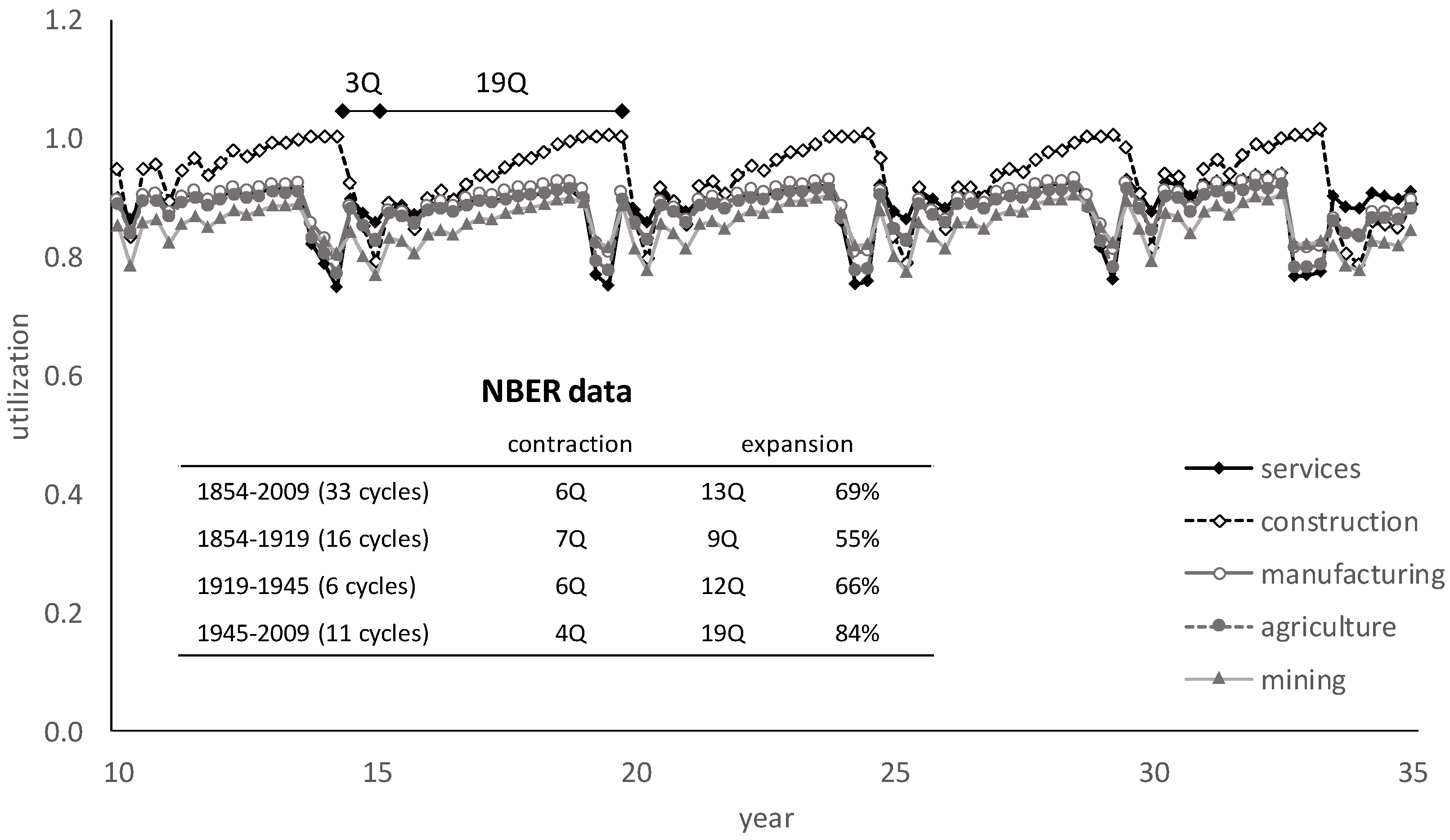
The coordinating role of the utilization ceiling in the model can be illustrated with an analogy to boats at a dock. When the tide is coming in, the boats are pushed against the dock. They line up, but not because they coordinate their movements; rather, it is because the dock prevents them from going further. When the tide goes out, each boat drifts away from the dock at a rate determined by the currents and eddies where it is located. The boats are no longer neatly lined up, but the disarray lasts only until the next time the tide comes in. The analogy is imperfect, because sectors are connected, even if they are not coordinated (to stretch the analogy, as a boat moved it would tend to entrain the other boats.) In the model, the ceiling in the multiplier-accelerator model periodically lines sectors up, like the boats at the dock. When the utilization ceiling is reached in one sector, investment is high but consumption plans are frustrated, leading to under-consumption in other sectors. The fall in consumer demand leads to a fall in utilization, which leads to a fall in investment demand, which is only turned around because the fall in investment is halted by the floor of capital depreciation. In the trough of the business cycle, some firms postpone investment, while others continue to invest in expectation of a recovery. If that investment is sufficient, utilization eventually returns close to normal levels. Investment increases with utilization, and the recovery turns into a boom that continues until the utilization ceiling is reached once again.

Firms’ expectations of future growth are informed by their experience of past growth, so as the business cycle is repeated, investment and consumption patterns gradually align. When the structure of the economy changes, those patterns are disturbed, but they eventually re-align over time if expectations of future growth are sufficiently buoyant (Kaldor 1957, p. 601) to push utilization rates to the ceiling. If they are not sufficiently buoyant, then the economy can go into a prolonged slump, with utilization rates falling to different degrees in different sectors. In the analogy to boats at a dock, this corresponds to the failure of the incoming tide. Without that coordinating force, the boats drift ever farther from the dock.

2.4. Wages

For wage setting, we adopt the Goodwin (1967) model, which ties changes in the real wage to labor productivity gains and unemployment. At normal levels of unemployment, wage rates rise at the same rate as productivity. They rise more slowly than labor productivity when unemployment is high and more quickly when unemployment is low. Unlike Goodwin, we express money wages in nominal terms. Wage raises are applied to current rates, followed by a cost of living adjustment that anticipates inflation. As it is difficult to negotiate a reduction in nominal wage rates, we apply the cost of living adjustment only if inflation is positive.

Specifically, the growth rate of the sector-specific wage w_i is given by

$${\widehat{w}}_i={\widehat{\lambda }}_i\left\{1+{\theta }_w\left[{\left(\frac{e_{-1}}{e_{\mathrm{ref}}}\right)}^2-1\right]\right\}+\max \left(\langle {\widehat{P}}_c\rangle ,0\right),\hspace{1em}e=\frac{L}{L_{\mathrm{LF}}},$$

(7)

where e is the employment rate, L is total employment, and L_LF is the size of the labor force. Here, P_c is the price level of consumption, so the cost-of-living adjustment applies an exponentially smoothed value for the inflation rate of consumption goods prices. When employment is equal to the reference level, e_ref, the wage rate rises at the same rate as labor productivity, plus a correction for expected inflation.

Each sector has some flexible and some inflexible labor. Flexible labor is laid off and re-hired over the course of a business cycle, while inflexible labor is maintained. Employed labor is drawn from and released into the labor force; that is, the working-age population that is participating in the labor market. The unemployment rate depends on the number of working-age people participating in the labor force. We assume the participation rate follows the unemployment rate with a lag. When unemployment is persistently high, job seekers become discouraged and exit the labor force. When unemployment falls, more of the working-age population is drawn into the labor force, but with a delay as they learn about changed conditions in the labor market, adjust routines at home, and refresh skills. In the model, this is represented by a dynamic participation rate ℓ, where

$$\Delta \ell ={\theta }_{\ell }\ell {(1-\ell )}^{a_{\ell }}\left(\frac{e}{e_{\mathrm{ref}}}-1\right),\hspace{1em}0<a_{\ell }\le 1.$$

(8)

The labor force is given by the participation rate multiplied by the working-age population.

2.5. Prices and Inflation

Most prices in modern economies are administered (Means 1935, 1972). This observation underpins post-Keynesian pricing theory (Lee 1999; Coutts and Norman 2013), in which most sectors are dominated by a few large firms (oligopoly) that set their prices as a mark-up on costs to generate profits. However, they do not have complete freedom because excessive profits encourage entry by rival firms. There is competition under oligopolies, but as price wars are damaging to all firms, it is mainly carried out on non-price dimensions such as reputation, new products or features, and customer relations.

In the model, total costs are equal to labor costs plus the cost of intermediate inputs purchased from other sectors. Tracking intermediate costs through the network of inter-sectoral exchanges, each sector’s costs can be expressed in terms of wage costs across its supply chains (Pasinetti 1973). Thus, wage costs ultimately determine prices. In the model, firms set a target price that would yield their target rate of return at previous-period costs,

$$p_i^{\ast }=\frac{{\kappa }_i}{{\kappa }_i-r_i^{\ast }}\left(w_{i,-1}{L}_{i,-1}+{\displaystyle \sum _{j=1}^N{A}_{ji}\cdot p_{j,-1}}\right).$$

(9)

In this expression, L_i is sectoral employment. Because most firms adjust prices rarely, we assume that at a sectoral level the observed price is a weighted average of the previous-period price and the target,

$$p_i=\left(1-{\xi }_i{\theta }_p\right)p_{i,-1}+{\xi }_i{\theta }_p{p}_i^{\ast }.$$

(10)

Here, the parameter θ_p is assumed to be the same for each sector, but there is a sector-specific correction ξ_i. Following Rowthorn (1977), we assume that firms have less flexibility to raise their prices when utilization is low, because they are more susceptible to competition. We therefore set

$${\xi }_i=\{\begin{array}{cc}\min (u_{i,-1}/u_{\mathrm{ref}},1)& ,\hspace{1em}{p}_i^{\ast }>p_{i,-1},\\ 1& ,\hspace{1em}{p}_i^{\ast }\le p_{i,-1}.\end{array}$$

(11)

Consumer price inflation is then calculated using Laspeyre’s index, as

$${\widehat{P}}_c\equiv {\displaystyle \sum _{i=1}^N\frac{p_i{F}_{c,i}}{{\displaystyle {\sum }_{j=1}^N{p}_j{F}_{c,j}}}{\widehat{p}}_i},$$

(12)

where F_c,i is household consumption of goods from sector i, while the GDP inflation rate is calculated using a similar expression, but with sectoral value added V_i replacing consumption,

$$\widehat{P}\equiv {\displaystyle \sum _{i=1}^N\frac{p_i{V}_i}{{\displaystyle {\sum }_{j=1}^N{p}_j{V}_j}}{\widehat{p}}_i}.$$

(13)

Inflation occurs when wages rise faster than labor productivity2. This introduces a circularity in the model. The wage-setting procedure described earlier and recorded in Equation (7) occurs in two steps: first, the intended real wage increases faster or slower than labor productivity depending on the unemployment rate; then a correction is added for anticipated inflation. But the reason inflation occurs in the first place is that wages rise faster than labor productivity.

The ultimate source of inflation in the baseline scenario is the unstable investment dynamics. During an expansion, there is increased demand for investment goods, and therefore labor, in the sectors that produce those goods. Those workers spend their incomes, generating demand for more goods, feeding the expansion and driving inflation. Because inflation ultimately comes from investment decisions, it can be moderated by influencing investment. This is accomplished in the model by tying the interest rate (which enters the investment function) to the inflation rate through the “Taylor rule” (after J. B. Taylor 1993). The real nominal rate of interest increases linearly with the GDP inflation rate and utilization in the manufacturing sector.

2.6. Consumption

A substantial amount of household expenditure is routine: locked in through contracts or the costs of operating durable commodities; constrained by the location of home, work, and school; or imposed by physiological necessity. In the 2014 US Consumer Expenditure Survey,3 two-thirds of all household expenditure was on housing, transportation, food, apparel, and related services. The implication is that less than half of expenditure is flexible in the short run, helping to stabilize the economy during the contraction phase of the business cycle. Over longer time scales, households expand their consumption as their incomes rise. In the model we capture the combination of long-run expansion and short-term inflexibility by assuming that a component of consumption expands with total wages at normal utilization, while a further component varies over the business cycle as realized wage income falls and rises.

We treat all consumers as a homogeneous group, so consumption depends on the total wage bill,

$$W={\displaystyle \sum _{i=1}^N{w}_i{L}_i}.$$

(14)

Sectoral employment is a combination of flexible and stable employment. Denoting the flexible fraction of sector i’s workforce by φ_i, sectoral employment can be expressed in terms of the labor needed to operate the capital stock K_i at full capacity,

$$L_i=\left[{\phi }_i{u}_i+\left(1-{\phi }_i\right)u^{\ast }\right]\frac{{\kappa }_i}{{\lambda }_i}{K}_i.$$

(15)

The flexible labor pool thus rises and falls with capital utilization, while the stable pool remains at the level needed for operation at the target level of utilization.

Households are assumed to anchor their consumption based on their wage income when capital utilization is at its normal level in all sectors. At that point, the wage bill is equal to

$$W_{\mathrm{norm}}={\displaystyle \sum _{i=1}^N{w}_i{u}^{\ast }\frac{{\kappa }_i}{{\lambda }_i}{K}_i}.$$

(16)

Households target a desired real consumption level F_c,i* that depends on the normal wage and the realized wage,

$$P_c{F}_{c,i}^{\ast }=W_{\mathrm{norm}}{f}_i^{\mathrm{base}}+\left(W-{\displaystyle \sum _{i=1}^N\frac{p_i}{P_c}{W}_{\mathrm{norm}}{f}_i^{\mathrm{base}}}\right)f_i^{\mathrm{marg}}.$$

(17)

Thus, households plan to purchase a base consumption basket that is proportional to the wage bill at normal utilization. They then look at what they have left over after subtracting the cost of that basket from their wage, and allocate part of their remaining income on a further, marginal, basket of goods. Households’ expenditure plans may be frustrated if some sectors are at full utilization, so their actual expenditure levels F_c,i may be less than they planned. When that happens, we assume that they reduce spending on goods from different sectors in a proportion ΔF_c, so that actual expenditure can be written

$$F_c=F_c^{\ast }-z\Delta F_c.$$

(18)

The difference between wage income and consumption expenditure is household saving, S, where

$$S=W-{\displaystyle \sum _{i=1}^N{p}_i{F}_{c,i}}.$$

(19)

2.7. Active and Inactive Capital

When the economy of a country or region fails, it is left with the shuttered buildings and sometimes the machinery of the businesses that had once provided employment. Those buildings and equipment are still accounted for as part of capital stocks through prior investment, but they are not simply underutilized in the trough of the business cycle. They are inactive, and might not be reactivated.

In the model, we account for inactive capital by moving some underutilized capital into an “inactive” category. When investment picks up again, some of that investment is met by reactivating inactive capital. Capital stocks follow a modified version of the perpetual inventory method,

$$K_i^{\mathrm{active}}=-\left({\delta }_i+d(u_i)\right)K_{i,-1}^{\mathrm{active}}+I_i^{\mathrm{tot}},$$

(20)

$$K_i^{\mathrm{inactive}}=-{\delta }_i{K}_{i,-1}^{\mathrm{inactive}}+d(u_i)K_{i,-1}^{\mathrm{active}}-\rho \frac{K_{i,-1}^{\mathrm{inactive}}}{K_{i,-1}^{\mathrm{inactive}}+K_{i,-1}^{\mathrm{active}}}{I}_i^{\mathrm{tot}},$$

(21)

$$I_i=\left(1-\rho \frac{K_{i,-1}^{\mathrm{inactive}}}{K_{i,-1}^{\mathrm{inactive}}+K_{i,-1}^{\mathrm{active}}}\right)I_i^{\mathrm{tot}}.$$

(22)

When utilization is above the normal level u*, no capital is deactivated. As utilization falls below the normal level, an increasing fraction is deactivated through the coefficient d(u_i). It gets added to the inactive pool, which then depreciates at the same rate as active capital. Investment demand I_i^tot is then met through new production I_i or by reactivating inactive capital.

In the baseline scenario, the fraction of inactive capital is negligible. It is more relevant to scenarios in which economic output grows much less quickly, or shrinks.

3. Results

The model described above has multiple, interacting dynamics. Many of them are stable when acting on their own, but operate with delays. Systems with these features typically show cyclical behavior. Other dynamics, such as population or labor productivity growth, are always pushing upward, while investment dynamics are locally unstable, but bounded by a ceiling and a floor. We populated the model using a combination of values based on US data, typical values from the literature, and values calibrated to give persistent business cycles in the baseline scenario.

3.1. Structural Change

In the model, labor productivity growth differs between sectors, while expenditure shares per unit wage and per unit of capital investment are held fixed. As a result, sectoral value added as a share of GDP is nearly constant in the baseline scenario, while employment shares change dramatically. When either labor productivity or expenditure shares (or both) change at different rates in different sectors, full employment is not guaranteed (Pasinetti 1981, p. 87). In the model, a long-run balance is maintained through interactions between employment, wages, prices, and productivity growth.

3.2. Business Cycles

The model produces asymmetric business cycles, as observed in the US economy. As shown in Figure 2, the business cycle in the model, as measured by utilization, falls rapidly (over 3 quarters) and then rises slowly (over 19 quarters). This compares favorably to the post-World War II business cycle average of 4 quarters of contraction and 19 quarters of expansion.4 In the terminology of Sichel (1993), the cycle in Figure 2 is both steep and deep. In fact, Sichel found evidence of steepness and deepness only for unemployment in the US, and not for other macroeconomic indicators. In our model, in its present form, capacity utilization, GDP, and unemployment move together, so the model must be extended if it is to explain different patterns in different variables.

A notable feature of Figure 2 is that no cycle is a precise copy of another, although they are qualitatively similar. Partly this is because the model advances in discrete time steps (it is calculated each quarter), but partly it is because the cycles result from multiple interacting processes, each with its own characteristic time scale. The cycle for construction lags the cycles in other sectors, because orders are placed for investment goods before they are actually built.5 In keeping with the “boats at the dock” analogy introduced in the methodology section, all sectors other than construction converge on a similar utilization rate close to the peak, but fall to different degrees in the trough and recover at different rates.

3.3. Long Waves

Underlying the business cycle are much longer cycles, of about 43 years. This is consistent with the period of Kondratieff (1979) long waves, which are estimated to last between 35 and 60 years (Metz 1992). The source of the waves in the model are the interactions between technological change, pricing, and employment and wages. Rising employment and wages drive labor costs up. Because prices respond after a delay, this shifts the distribution of income away from profits and towards wages, stimulating labor productivity growth and dampening capital productivity growth. This combination reduces pressure on employment and wages, but also drives the profit rate down. Firms respond by raising their mark-ups, driving the income distribution towards profits and away from wages, encouraging faster capital productivity growth and slower labor productivity growth. The cycle then repeats. Consistent with observation, capital productivity changes over time, but has no clear trend as the capital productivity growth rate cycles around a value of zero.

3.4. Model Behavior in Alternative Scenarios

As discussed in the introduction, we contrast downshifting, or reducing working hours, with a reduction in consumption without reducing labor. In each scenario, we represent a transition as a change in a model parameter that starts in year 100 (to allow some transient behavior to work itself out) and continues for 25 years. We chose values that pushed the model close to a critical level, or just beyond it, so they are much more substantial than actually observed consumer initiatives. In a downshifting scenario we reduce the effective size of the working age population by 40% over the time period, which leads temporarily to no GDP growth. In two reduction scenarios we reduce consumption per unit wage by either 7.5% or 15% over the same time period. In the former scenario the economy continues to expand, while in the latter it enters a deep slump.

In the following set of graphs we show the model behavior between years 75 and 150. The labor force is shown in Figure 3. The effect of reduced working hours in the downshifting scenario is evident in the figure. In the 7.5% reduction scenario, employment rises above the baseline after a delay, while it falls off precipitously in the 15% reduction scenario.

The effect on consumption is shown in Figure 4. Relative to the baseline scenario, consumption rises slightly in the downshifting scenario before it drops gradually to less than half the baseline level. In the 15% reduction scenario, consumption falls as the economic engine fails. In contrast, in the 7.5% reduction scenario, consumption not only recovers: it overshoots relative to the baseline.

The trajectory of GDP in the scenarios is shown in Figure 5. As seen in the figure, GDP does not grow in the downshifting scenario between years 115 and 135. After that it begins to pick up again. The 10-year lag between the reduction in work hours and the flattening of GDP is a result of multiple interacting dynamics in the model. In the 7.5% reduction scenario, GDP, like consumption, actually rises above the baseline level for a time, while GDP collapses in the 15% reduction scenario.

The downshifting scenario drives inflation, as seen in Figure 6. This effect, which was anticipated by Rezai et al. (2013), happens because firms are unaware of the cultural phenomenon of downshifting and are making their investment and production plans based on past experience. Because less labor is available, it pushes wages up sharply. In contrast, when consumption is reduced without withdrawing labor in the two reduction scenarios, inflation falls below baseline. This deepens sharply in the 15% reduction scenario, and recovers and then overshoots in the 7.5% reduction scenario.

Higher labor costs in the downshifting scenario stimulate investment in labor-saving technology, again as anticipated by Rezai et al. (2013). The effect can be seen in the graph of manufacturing labor productivity growth shown in Figure 7. The result is an increase in the capital-to-labor ratio, as shown in Figure 8. That is, in the downshifting scenario, as employment and output fall, the economy shifts towards labor-saving and more capital-intensive forms of production. The result is that the capital stock continues to expand, even as GDP growth stagnates, albeit at a slower rate than previously.

4. Discussion

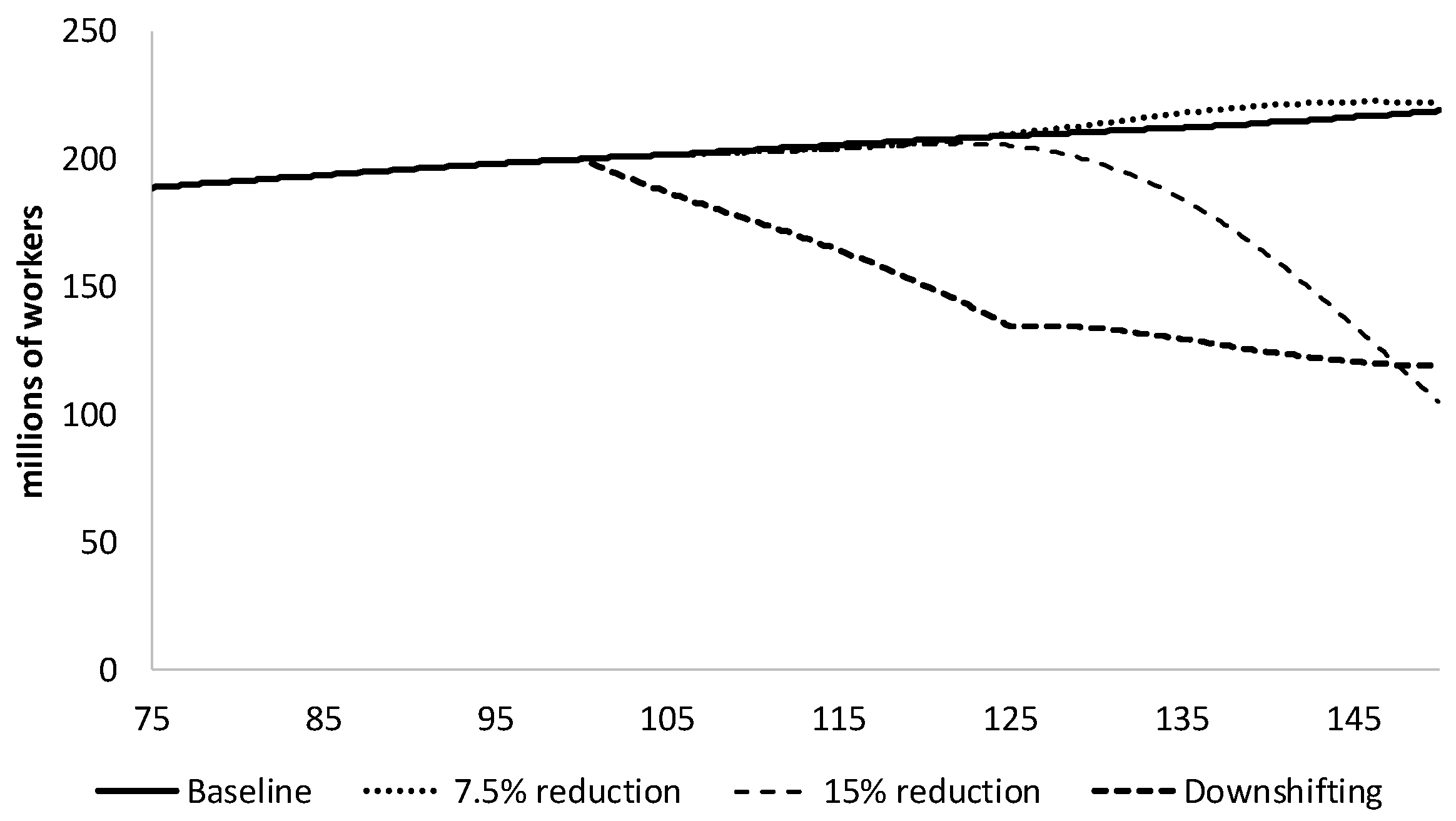
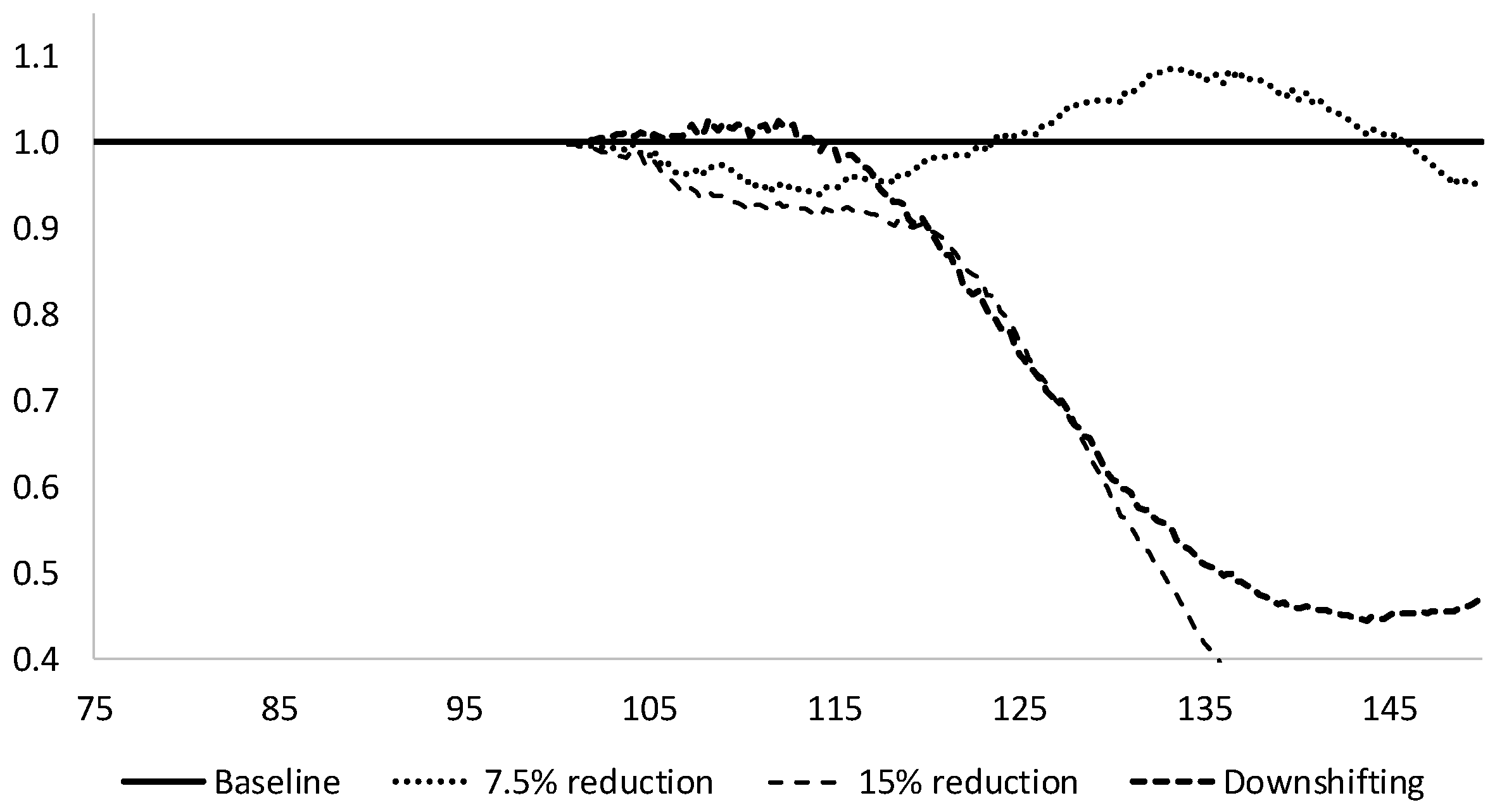
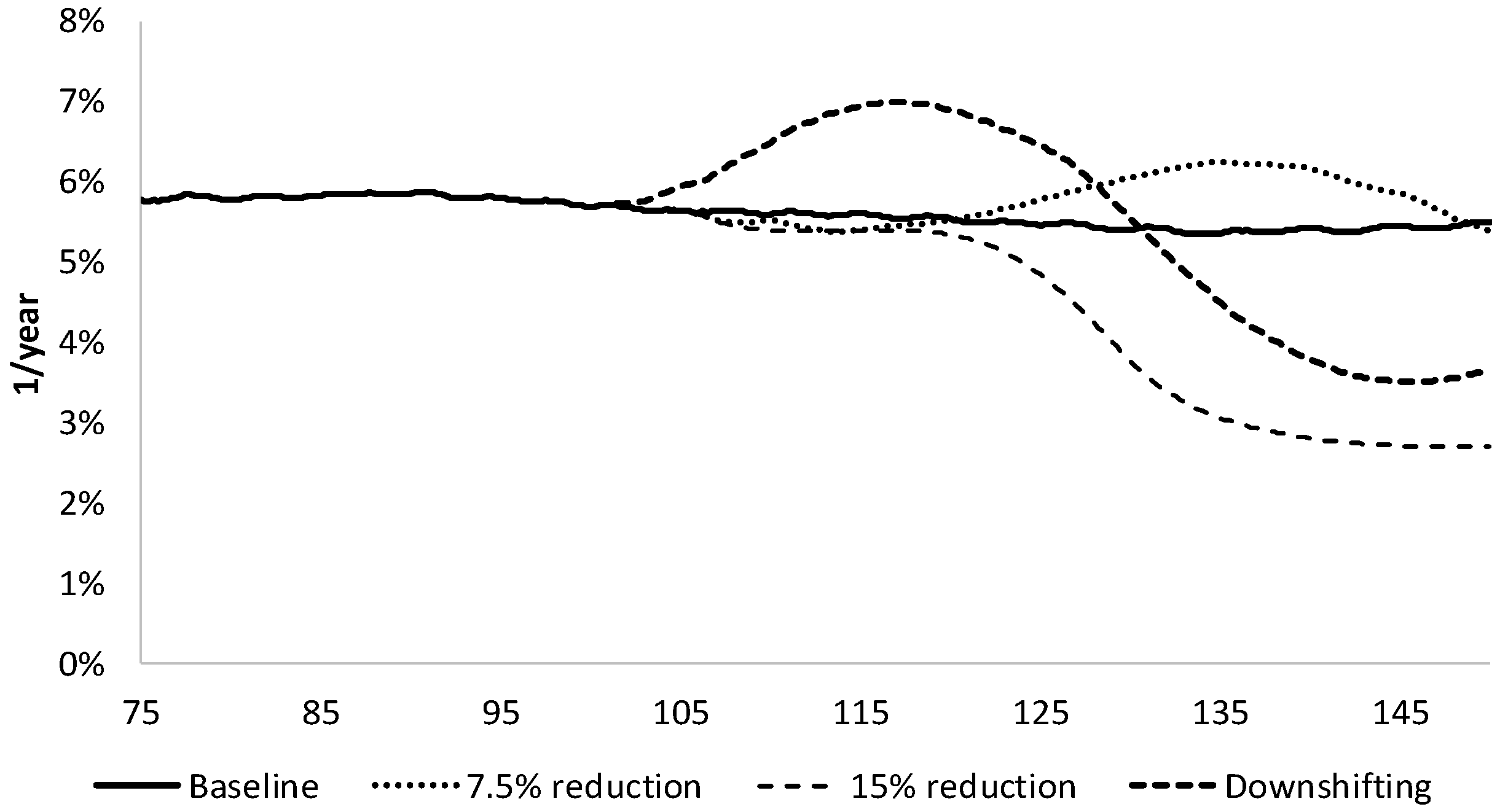
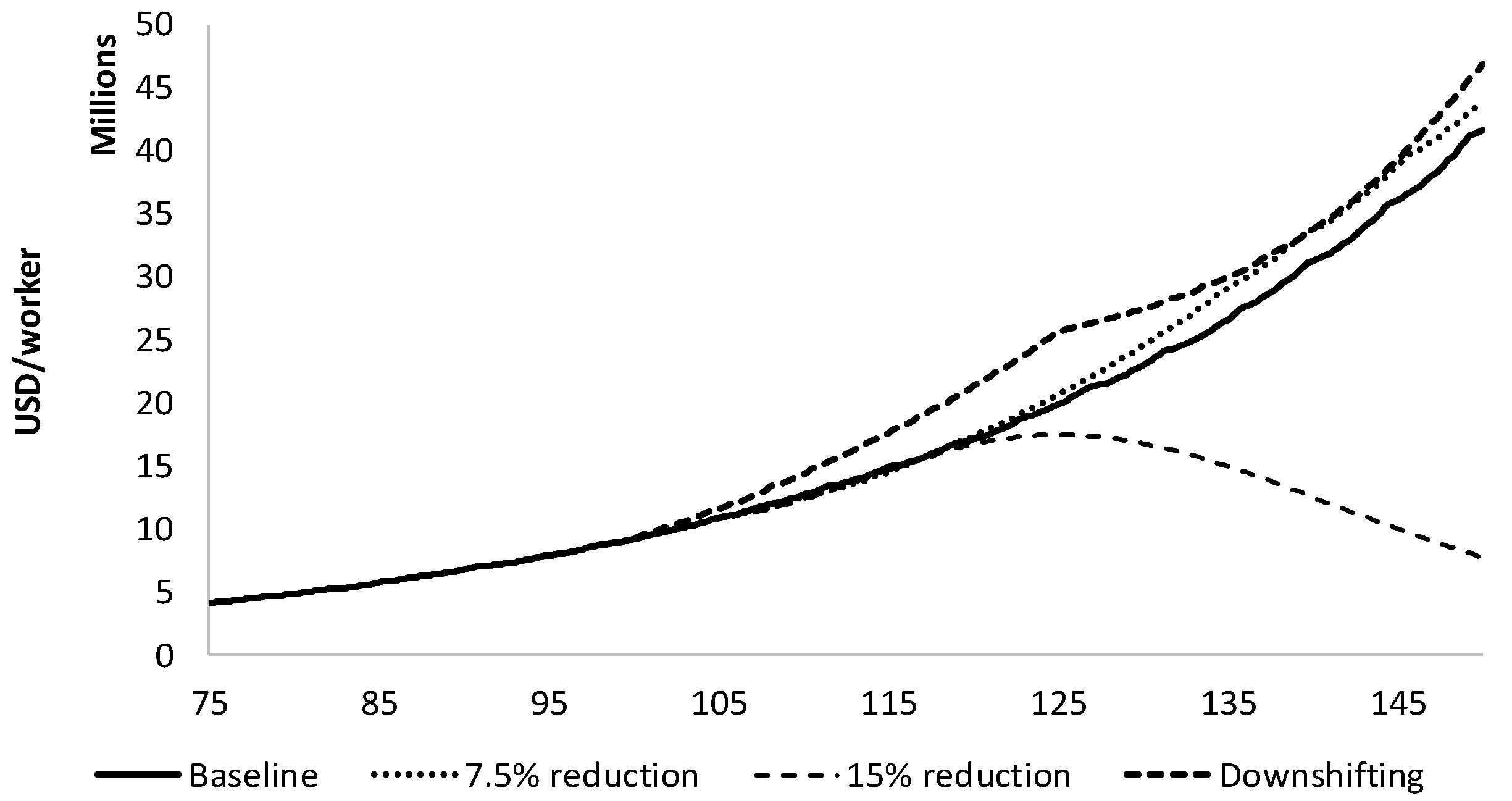
In an economy out of equilibrium, the sequence of events matters. In an equilibrium model, reduced consumption and reduced wage income happen together, whereas in a disequilibrium model with delayed feedbacks it takes time for the system to accommodate the change, and actions may not have their intended effects. In the disequilibrium model presented in this paper, reducing consumption without reducing working time either has no net effect—the economy recovers and cycles around the baseline trajectory—or it leads to a worsening contraction. In contrast, if workers reduce their working time, then the economy can slow significantly without collapsing.6

The model results shed some light on debates in ecological economics around the causes of economic growth. Fractional reserve banking is not a driver of growth in this model (see (Fontana and Sawyer 2016) for a thorough discussion); our treatment of business investment is consistent with a “horizontalist” position on money and banking (Lavoie 2011), in which the central bank is free to set an interest rate, while commercial banks offer businesses the credit they demand. Furthermore, without a financial sector, financialization is not driving unsustainable growth in the model (but is likely to be important; see Jerneck 2017). Instead, growth is driven by the prospects for business income. When those prospects are rosy, the economy tends to grow, and when they wither, the economy can falter and even slide towards collapse.

The model has some limitations. A low-carbon transition must involve citizens, their government, the private business sector, and trading partners, while the model presented in this paper is of a closed economy without a government sector, and in the scenarios we presumed that only households take the initiative. For the particular mechanism explored in this paper, these limitations are not as relevant as they would be in a full analysis. We examined consumer-led efforts to reduce working time and expenditure, independent of any government initiatives. Furthermore, by abstracting from the government and trade, we could study the potential rebound from downshifting, as identified by Rezai et al. (2013). We did, indeed, observe some rebound as a smaller labor pool drove up wages, which then drove consumption expenditure and labor-saving technological innovation. However, the rebound in expenditure and output was less than the initial reduction.

A more relevant limitation for the mechanism explored in this paper is that we represent labor by number of employees, rather than by hours of work. Downshifting typically involves reduction in work hours, rather than full withdrawal from the labor force. For the present analysis, we justify this treatment by assuming that the labor force represents “effective workers” expressed in full-time equivalents. However, in reality the productivity and compensation of one full-time worker generally differs from that of two half-time workers. Future analyses would benefit by disaggregating both labor and households.

Finally, in future work we will expand the behavioral rules that consumers might follow. The model assumes that expenditure varies with wage income. That may be true as incomes rise, but households that are downshifting may try to maintain their consumption by spending down savings, which would tend to sustain GDP. To implement this assumption, the model must track savings, which it does not do at present.

These considerations aside, the results suggest that households can, at sufficiently large scale, effect significant change in the absence of private sector or government action. The model takes an aggregate view of the economy, as suggested by Rezai et al. (2013). The results support Schor’s (Schor 2005) contention that reducing work hours can be an effective strategy in reducing the footprint of high-income households.